Article

Evaluation of Different Methods to Assess the Hydraulic Behavior in Horizontal Treatment Wetlands

by
Feliciana Licciardello
1,
Alessandro Sacco
2,
Salvatore Barbagallo
1,
Delia Ventura
1 and
Giuseppe Luigi Cirelli
1,*
1
Dipartimento di Agricoltura, Alimentazione e Ambiente (Di3A), Università degli Studi, di Catania, 95123 Catania CT, Italy
2
International Doctorate in Agricultural, Food and Environmental Science-Di3A, University of Catania, 95123 Catania CT, Italy
*
Author to whom correspondence should be addressed.
Water 2020, 12(8), 2286; https://doi.org/10.3390/w12082286
Submission received: 16 June 2020 / Revised: 20 July 2020 / Accepted: 11 August 2020 / Published: 14 August 2020

Abstract

:
While there have been numerous studies on the rate and development of clogging in horizontal subsurface treatment wetlands (HSTWs) and, consequently, the effects on its hydraulic characteristics, research has not shown a clear understanding of the processes. The existing methods for measuring the impact of clogging provide limited information on the extension and degree of the phenomenon. This study aimed to evaluate the capacity of various measurement techniques to assess the degree and variation in space and time of clogging in HSTWs. Hydraulic conductivity at saturation (Ks) measurements were conducted using a newly implemented scheme, the drainage equation method, and traditional tracer tests, which were carried out in a full-scale HSTW system, located in Sicily, Italy, during 2019. After five years of operation, the results highlighted a severe decrease in Ks (<1000 m day−1) in the inlet zone (despite the fact that the filter gravel was replaced in 2017), a very high reduction of Ks along the central path inside the bed, a nonuniform flow through the HSTW, the presence of stagnant zones, and a reduction of the porosity of the bed gravel. Nonetheless, the mean values of the physical–chemical and bacteriological parameters at the hybrid treatment wetland (hybrid TW) outlet indicated that the partial clogging had no significant effect on the quality of the discharged water. Moreover, the results obtained using the different measurement techniques (in terms of both the Ks values and the flow distribution inside the bed) were consistent with each other and with results obtained previously for the same system. Finally, the most efficient combination of methods to assess clogging in HSTWs was identified.

1. Introduction

Bed clogging of horizontal subsurface treatment wetlands (HSTWs) is inevitable and not a new phenomenon. Its development and impacts on the design and operation of these systems must be taken into account to avoid reductions of their lifetime [1,2,3]. Clogging is also a complex phenomenon, because sets of mechanisms act differently during the lifetime of HSTWs [4]. Cleaning the bed media in the inlet zone of HSTWs (where microbial biomass formation primarily occurs) may be unavoidable and should be regularly scheduled. On the other hand, designers have to take into account that the clean-bed hydraulic conductivity at saturation (Ks) will change significantly once the system is put into operation and that HSTWs must nonetheless be able to operate efficiently. The Ks value, which is largest at start-up, will decrease with time as plant roots, microbial biofilms, and chemical precipitates gradually occupy spaces. While there have been numerous studies on the rate and development of clogging and, consequently, on the changes to the hydraulic characteristics of HSTWs, research has not acquired a clear understanding of the processes [5]. In addition to techniques that measure the properties of clog matter (elucidating the nature and the degree of clogging) [6,7] and tomography (allowing for the production of a 3D image of the distribution of the clogging and its concentration in the filter) [8], all the other approaches are based on the evaluation of HSTW hydraulic behavior. In particular, one of the main effects of clogging is a reduction of the hydraulic conductivity (Ks) at saturation of the porous media [9,10,11]. The Ks values at saturation can be obtained by surveying the hydraulic gradients between points in the filter media and then applying Darcy’s law [12,13,14]. A limitation of this method is that the reliability of the determined Ks values depends on the accuracy of the hydraulic gradients [12].
Ks measurements can be made by falling- and constant-head tests, which were specifically developed to detect the potentially high hydraulic conductivity of wetland gravels [15,16]. In particular, the in situ falling-head method, used by [7,8] to determine the Ks in several HSTW beds, is based on the Naval Facilities Engineering Command Design manual [17]. The equation that is used for the determination of Ks depends on the geometry of the cavity (that is, the ratio between the radius R and length L) and, consequently, of the chosen scheme [17,18]. A disadvantage of these methods is that they require numerous point measurements inside the bed (to measure the vertical Ks) and also along a vertical profile (to determine the horizontal Ks), if an impervious permeameter is used. The latter limitation was recently overcome by the implementation of a pervious permeameter with a calibrated equation to consider the effect of clog matter on the horizontal direction of flow and also to save time [18]. It should be noted that these methods involve a certain degree of disturbance due to the insertion of the tube into the substrate [19]. A synthetic Ks value for HSTW beds can be obtained by simulating the measured outflow through an equation developed in [20] to predict the cumulative drainage volume from aquifers overlying sloping, impermeable layers. The Ks values obtained using the drainage equation were validated by a comparison with values obtained by Darcy’s law in four rock-reed filters filled with different substrates (from 2 to 4 cm in a sand and gravel mixture) and either planted with Phragmites australis or unplanted [12]. A disadvantage of this method is that the system must be stopped during the experiment, and the stoppage can last up to several days for large HSTWs. The hydrodynamic visualizations obtained through tracer tests can also allow for the study of the effect of clogging phenomena on the flow in a porous medium, e.g., using sodium chloride (NaCl), rhodamine dye, or potassium bromide [21,22,23]. Tracer tests can be conducted both at the outlet of the system or at various points inside the bed to obtain different information. The clogging impacts on the hydraulics of the whole bed can be investigated by monitoring the tracer passage through the outlet [24], while the measurements inside the bed are required in order to identify preferential flow paths and, eventually, possible causes of clogging [22].
While there are different available approaches, numerous research reports indicate that no individual method could quantitatively assess clogging phenomena in HSTWs [19,23,25]. To better monitor the clogging evolution in HSTWs, different combinations of approaches are suggested. In [25], Ks measurements, the quantification of clog matter, and tracer tests (NaCl) are combined for full-scale investigations into HSTWs. In [23], Ks measurements, tracer tests (NaCl), and geophysical techniques are integrated to highlight a progressive increase in clogging in a full-scale HSTW in Sicily. The latter is a hybrid treatment wetland (hybrid TW) system that functions as a secondary wastewater treatment system of the IKEA® store, located in the industrial district of Catania, Sicily, Italy. Because Ks measurements and tracer tests highlighted a partial clogging in January 2017, a restoration measurement was carried out in the inlet zone of the HSTW bed in April 2017. Since there is no single method that can quantitatively measure the clogging in HSTWs [19], and due to the fact that each has different advantages and disadvantages, it can be useful to identify an approach, or eventually a combination of approaches, that allow for a complete understanding of clogging development in a treatment wetland in the most time-efficient and easily repeatable way.
This paper aims (1) to assess the degree and variation in space and time (also by comparison with previous experimental campaigns) of clogging in the HSTW system functioning as a secondary wastewater treatment system of the IKEA® store, and (2) to identify the most efficient way to evaluate the phenomenon in HSTW systems. In order to reach these objectives, an experimental campaign integrating traditional and innovative methods to assess the hydraulic behavior in HSTWs was carried out in the horizontal bed of the hybrid TW system of the IKEA® store, which had already been partially clogged in the past. In particular, traditional tracer tests were compared with Ks measurements in a newly implemented scheme (i.e., by using a pervious permeameter with a calibrated equation) and the drainage equation method. To ensure that the HSTW conditions were the same, the three methods were carried out consecutively in February 2019; it was not possible to perform them simultaneously due to the characteristics of the individual methods.

2. Materials and Methods

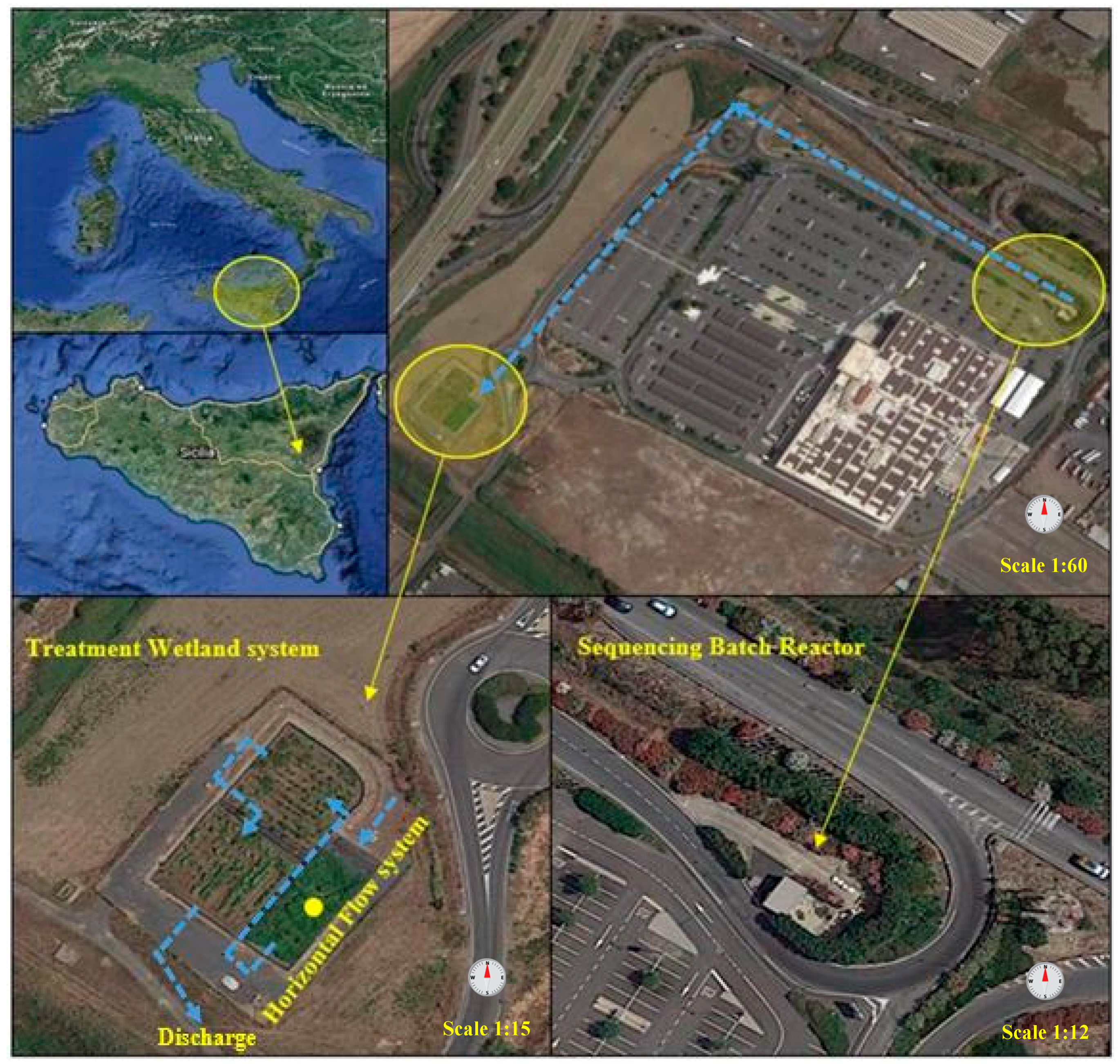
2.1. Full-Scale HSTWs Characterization

The selected HSTW was chosen as a case study to assess clogging using various measurement techniques. The HSTW system is part of the hybrid TW system that functions as a secondary wastewater treatment system for the IKEA® store, located in the industrial district of Catania, Italy (37°26′54.2″ N 15°02′05.2″ E, 11 m a.s.l., Figure 1). The area is semiarid and characterized by average annual precipitation of about 760 mm. The values for temperature and humidity were in the range of 1.6–40 °C and 8–100%, respectively, in 2018. The average monthly precipitation was 55 mm during January and February 2019. No rains occurred in the days during which the measurements were made or on the three previous days. The treatment plant includes a screening unit and a sequential batch reactor (SBR) as the primary treatment. The SBR was designed for treating wastewater produced by toilets and the food area of the store, with a maximum flow rate of 30 m3 day−1 (two batch phases every 12 h) and total nitrogen (TN) load of 135 mg L−1. The IKEA® store and the Department of Agriculture, Food, and Environment of the University of Catania have been in charge of running and monitoring the HSTW, respectively, from the time of the installation. Because of the high fluctuations of the flow and TN [23], the primary treatment was integrated with a hybrid TW in 2014. The system includes three in-series connected beds: HSTW, which allows for a reduction of organic matter and suspended solid (SS) concentrations, followed by two vertical subsurface flow TWs (V1-TW, V2-TW), which are designed to remove the wastewater organic matter, SS, and to further nitrify ammonia to nitrate. The HSTW bed has a surface area of about 400 m2 (12 × 34 m), and is filled with 0.8–1.5 × 10⁻² m of volcanic gravel to a depth of 0.60 m.
The porosity and Ks values of the original clean gravel were 0.41 and 19,466 m day−1, respectively [18]. The HSTW, planted with Phragmites australis, is fed discontinuously with a daily effluent from the SBR plus effluent from the screening unit, which does not include the SBR, when the wastewater produced in the IKEA® store exceeds a flow rate of 2.5 m3 h−1. Based on the total wastewater produced by IKEA, the annual volume of untreated wastewater feeding the HSTW was, on average, around 30% of the total volume, while during weekends and holidays, the daily volume of untreated wastewater (WW) was up to 50% of the total daily volume amount. Due to the high volumes of WW produced at the IKEA® store at the end of 2016, the SBR was often bypassed, and a high organic load entered the hybrid TW system. Thus, it was already necessary to remove and replace the filter gravel close to the inlet area after three years of operation (in April 2017). A CR-1000 automatic weather station (Campbell Scientific, Logan, UT, USA) was installed close to the experimental plant to measure the temperature, wind speed and direction, rainfall, global radiation, and relative humidity. The vegetation harvest was carried out every year (at the end of January or at the beginning of February). During the investigation campaign, the vegetation groundcover was about 85%. In particular, the plant density was low in the area close to the inlet and, in some regions, randomly distributed along the middle path. For more details on the hybrid TW, see [23].

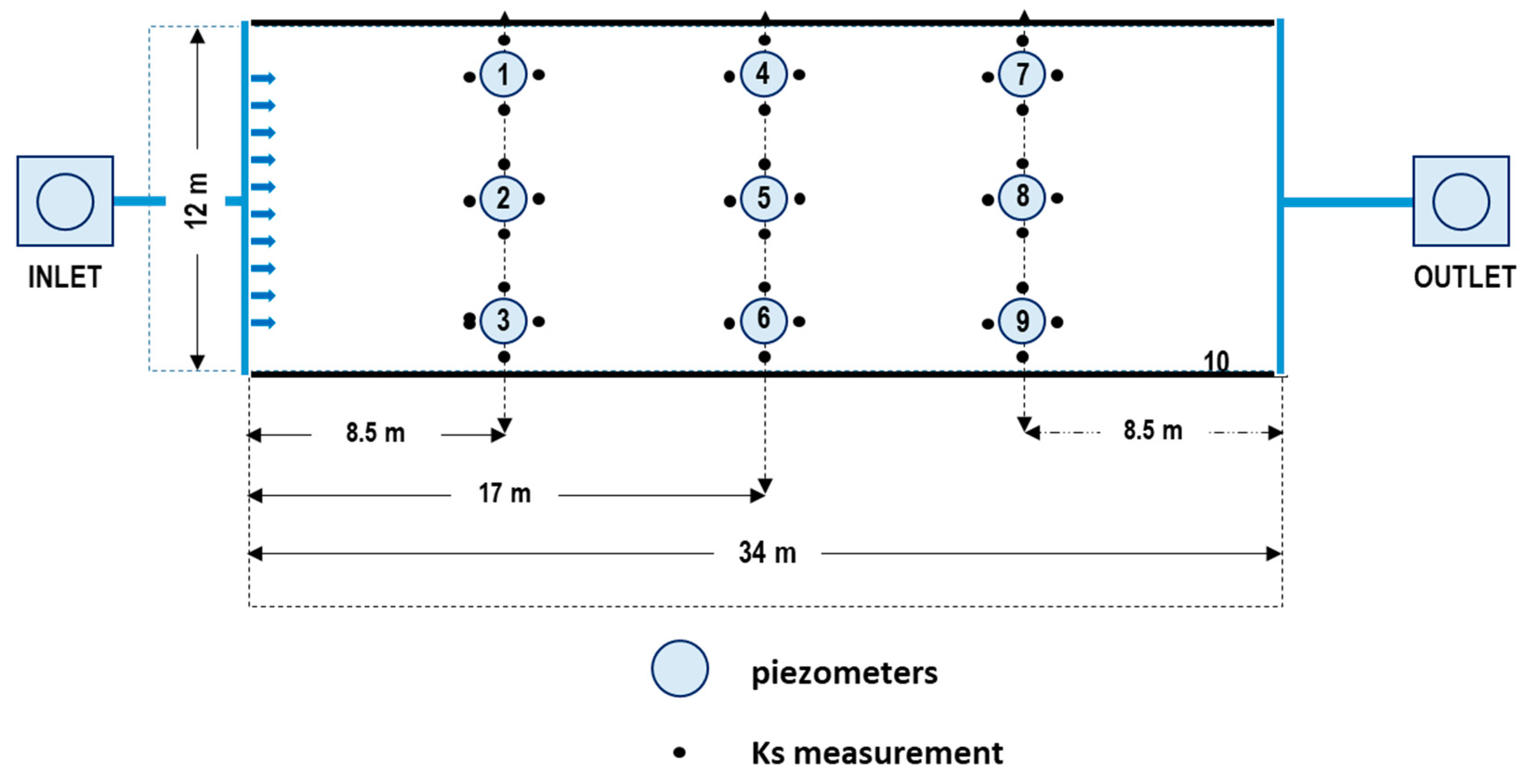
2.2. Ks Measurements in the Full-Scale HSTW Bed

The falling-head method was applied to determine the Ks values in the HSTW bed in February 2019. In particular, four falling-head infiltration tests were performed around each of the nine piezometers located in the bed (Figure 2) at the same depth (see Table 1). Two open-ended tubes, one impervious (IMP) and one pervious (P), and the corresponding equations adapted from [17] to various applicability conditions (Table 1) were used. In particular, the IMP permeameter (Table 1, Scheme 1, also known as the Standpipe) allowed us to evaluate the vertical Ks values using Equation (1). For isotropic gravels (clean or not clogged), this would not be a problem. However, given that the clogging process is likely not to be isotropic, the vertical Ks values obtained using this method could be different from the horizontal Ks values. Instead, the P permeameter (Table 1, Scheme 2) allowed us to evaluate both vertical and horizontal Ks, using Equation (2), as in [18]. Both schemes did not require drilling a borehole, as the pipe was merely pushed directly into the substrate. This saved time, compared to other schemes, and also minimized disturbance to the porous medium. Equation (1) is the following:
K s = 2 π R + 11 L 11 ( t 2 t 1 ) ln ( H 1 H 2 )
where R and L are the radius and the submerged length (m) of the tube, respectively, as defined in [17]; and H1 and H2 are the water levels (m) in the permeameter cell corresponding to time t1 and t2 (s), respectively. Equation (2) is the following:
K s = 2 π R m o d + 11 L m o d 11 ( t 2 t 1 ) ln ( H 1 H 2 )
where Rmod and Lmod are the radius (m) and the submerged length (m), respectively, as calibrated in [18]; and H1 and H2 are the water levels (m) in the permeameter cell corresponding to time t1 and t2 (s), respectively.
A small hole was dug in the granular medium to reach the water table, and then the permeameter was inserted using a mallet. A plastic water reservoir (6.6 L volume) with measurement units was assembled together with a ball valve to add water in a single-pulse mode, as required. A pressure probe (Sensor Technik Sirnach (STS), AG, Sirnach, Switzerland), connected to a laptop by means of a CR200-R (Campbell Scientific) data logger, was used to measure the variation of the water levels (H) within the measurement unit. A driver was added to the device to allow for the insertion of the pressure probe inside the steel permeameter (Table 1). The pressure value at atmospheric pressure was checked before each measurement started. Four water level data per second were recorded for a duration of 30 s. The decrease in the water height inside the permeameter was monitored until the water reached the static water table. The best fit between the simulated and measured water levels was obtained by summing and minimizing the squared differences between the theoretical curve and that obtained in the field, following Equation (3):
t = 0 n = ( H o b s ( t ) H s i m ( t ) ) 2
where Hobs is the height of the water table level measured inside the permeameter at time t during the test (m); and Hsim is the corresponding modeled data calculated by Equation (1) or Equation (2) (see Table 1), depending on the scheme used.
This condition allowed us to estimate the value of Ks using an iterative, nonlinear procedure that makes use of the Excel Solver spreadsheet plug-in (Frontline Systems, Incline Village, NV, USA).

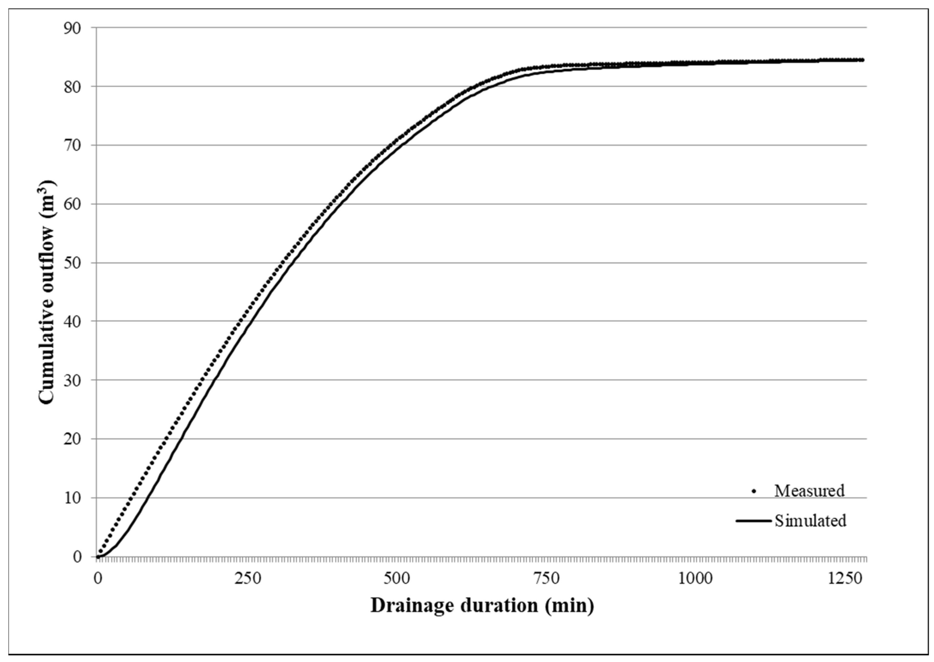
2.3. Drainage Experiment

The drainage equation proposed in [20] and applied to HSTWs in [12] was used to find a synthetic Ks for the whole HSTW bed. The equation has the following form:
V = V * ( 1 exp ( t 3 h ( 0 , 0 ) K s cos β s L 2 ( 1 V * V i ) ) 1 V * V i exp ( t 3 h ( 0 , 0 ) K s cos β s L 2 ( 1 V * V i ) ) )
where
  • Vi = swLh (0, 0) (m3) (initial volume of water for x = 0 and t = 0);
  • V* = s ∙ w ∙ L ∙ (h (0, 0)–h (0, t)) + ½ sw ∙ L2 ∙ tan β (m3) (potential outflow due to drawdown and to the slope);
  • V = cumulative drainage volume at any time (m3);
  • s = drainable porosity (m3 m−3);
  • x = linear distance from the drain (m);
  • t = time at which the drainage volume is calculated (s);
  • β = slope of the impermeable layer (m m−1);
  • L = length of the bed (m);
  • w = width of the bed (m);
  • Ks = saturated hydraulic conductivity (m min−1);
  • h (0, 0) = hydraulic head at x = 0 and t = 0 (m); and
  • h (0, t) = hydraulic head at x = 0 and t > 0 (m).
Ks (m min−1) is the only unknown term in the above equation, when applied to the drainage experiments. Measured cumulative drainage volume data were obtained first by closing the inflow and outflow valves to produce a horizontal water table and then by opening the outlet valve and collecting the drainage volume in a tank. The inflow valve remained closed for the whole duration of the test. The variation of the water levels within the tank was measured by the pressure probe positioned in the tank and connected to a laptop, as described above. The water level data, recorded inside the tank every 5 min, were converted into drainage volumes. The drainage experiment was carried out once in February 2019. A range of conductivity values were applied to Equation (4), until the resulting outflow curve matched the measured outflow. The value of Ks that produced the closest fit and gave the simulated cumulated outflow closest to the measured one was taken as the hydraulic conductivity of the substrate for the particular drainage test.

2.4. Tracer Tests

A tracer test was conducted in February 2019 by introducing an impulse of NaCl into the HSTW inlet at time zero. NaCl was chosen for its efficiency and low-cost characteristics, but also because it is not organic, and it was already successfully used in the same system [23]. The amount of tracer (32 kg 100 L−1 for a total volume of 200 L and a pulse duration of about 10 min) was chosen in order to reach an average benchmark concentration at least ten times that of the background concentration, as suggested in [26]. The measured EC (μS cm−1) values, after subtraction of the background value (between 1600 and 1800 μS cm−1), were then converted into NaCl concentrations (mg L−1) by a linear calibration curve (R2 = 0.99). The pumping discharge of the solution was the same as the normal water flow in the HSTW system. The solution was prepared in a bucket, in which the tracer was added and mixed until a uniform concentration was reached. A pulse-inject of the tracer solution was then added with a pump into the inlet zone of the HSTW system. The fluid electric conductivity (EC) was measured by ten conductivity probes (delta OHM–HD 2106.2, DeltaOhm, Padova, Italy). One of them was located at the outlet, and the others were located inside the nine piezometers in the HSTW bed. The EC data were recorded by each probe every 15 min. The HSTW outflow volumes were measured using a flow measurement device for the whole test. No rain occurred during the test.
The NaCl injection into the HSTW inlet provided information about the efficiency and detention times in the system. In fact, in ideal flow patterns, the water particles move at the same velocity, reaching the outlet together. In this case, a tracer impulse would also exit as an impulse (a sharp spike of concentration). It is clear from numerous studies that TWs are neither plug flow nor well mixed, and due to preferential flow channels, vertical stratification occurs in gravel beds, with more significant flows arising at lower levels in the system [27,28,29]. Thus, also in the present case, the response to the impulse tracer input was a time-delayed, bell-shaped curve, called the retention time distribution (RTD). Thus, the analysis of this curve allowed for the derivation of critical parameters characterizing the hydraulic behavior of the system.
First, it was necessary to evaluate the validity of the test, checking that the tracer was recovered nearly in its entirety at the wetland outlet. To achieve this, the relative tracer mass recovery (%) was calculated as
M o u t M i n   × 100
where:
  • Mout is the total recovered tracer mass at the outlet (g);
  • Min is the total tracer introduced into HSTW (g); and
  • Mout was determined in accordance with [30]:
M o u t =   0 Q ( t ) · C ( t )   dt
where
  • Q(t) is the outflow rate at time t (m3 h−1);
  • C(t) is the tracer concentration at time t at the outlet (mg L−1); and
  • t is the sample time (h).
Then, the retention time distribution (RTD), which represents the various time fractions of the water spent in the reactor and hence the contact time distribution for the system was analyzed.
In general, the RTD is the probability density function for the residence times in a wetland. For an impulse input of a tracer into a steadily flowing system, the time function is defined by
E ( t ) =   Q   · C ( t ) 0 Q   · C ( t ) dt   =   C ( t ) 0 C ( t ) dt
The first numerator is the mass flow of the tracer in the wetland effluent at any time t, after the time of the impulse addition. The first denominator is the sum of all the tracers collected and should thus equal the total mass of the injected tracer.
Thus, the mean tracer detention time (tm) is presumed to be the actual mean detention time and can be calculated as the first moment of the curve (the centroid of the C-curve) as
t m =   0 t   ·   C ( t ) dt 0 C ( t ) dt
where t is the sample time that, after the definition of the probability density function, can be expressed as
t m =   0 t   ·   E ( t ) dt 0 E ( t ) dt
A wetland may have internal excluded zones that do not interact with the flow [4], such as the volume occupied by biomass (roots, rhizomes, etc.). In a steady-state system without excluded zones, the tracer detention time (tm) equals the nominal residence time (tn), which is defined as
t n = V Q
where
  • V (m3) is the volume of the water in the system; and
  • Q (m3 h−1) is the water flow rate through the system.
Following [31], a parameter for evaluating the hydraulic efficiency of the system can be simply defined as
λ = t p t n
where tp is the time that the maximum concentration of tracer occurred (h). This measure has the advantage of being readily derived from the RTD, and it does not have the problem related to the calculation of tm [31]. The hydraulic efficiency can be considered good if λ > 0.75; it is satisfactory if 0.5 < λ < 0.75; and it is poor if λ ≤ 0.50.
A second parameter that can be determined directly from the residence time distribution is the variance (σ2, Equation (12)) (or the square of the standard deviation):
σ 2 =   0 ( t t m ) 2   ·   C ( t ) 0 C ( t ) dt
where σ 2 is the second moment of the curve and characterizes the spread of the tracer response curve concerning the mean of the distribution (tm).

2.5. Wastewater Quality Characterization

Wastewater quality was monitored one/two times per month, from April 2016 to February 2019. The sampling points were located at the hybrid TW inlet and at the three outlets of each TW bed (HSTW, V1-TW, and V2-TW). Standard methods [32] were applied for wastewater quality analysis, which included total suspended solids (TSS, mg L−1) at 105 °C, biological oxygen demand after five days (BOD5, mg L−1), chemical oxygen demand (COD, mg L−1), phosphate (PO4, mg L−1), ammonia nitrogen (N-NH3, mg L−1), total nitrogen (TN, mg L−1), nitrate nitrogen (N-NO3, mg L−1), and Escherichia coli (E. coli, CFU 100 mL−1). In order to characterize the HSTW influent, the following parameters were calculated [2].
The maximum areal organic loading rate (OLR) (g BOD5 m−2 day−1) is defined as
O L R = B O D 5 A
The hydraulic loading rate (HLR) (mm day−1) is defined as
H L R = Q A
The total suspended solids rate (TSSLR) (g TSS m−2 day−1) is defined as
T S S L R = T S S A
where
  • Q (m3 day−1) is the water inflow rate through the system;
  • TSS (g day−1) is the amount of TSS, based on the water inflow rate through the system;
  • BOD5 (g day−1) is the amount of BOD5 based on the water inflow rate through the system; and
  • A (m2) is the wetland surface area.

3. Results

3.1. Ks Measurements in the Full-Scale HSTW Bed

Table 2 and Figure 3 report the Ks mean values (indicated as Ks values below) around each of the nine piezometers inside the HSTW bed and their standard deviation (SD) observed in 2019 and in the previous campaign [18]. The Ks values measured in piezometer 1, 2, and 3, located in the first transect close to the inlet, were the lowest. A very low Ks value was also observed in piezometer 8 (Table 2 and Table 3). Consequently, in 2019 the lowest values of Ks were observed in the inlet transect (660 m day−1) (Table 3) and along the middle path (3682 m day−1) (Table 4). The Ks values found along the transects located in the middle part of the bed and close to the outlet were similar (Table 3).

3.2. Drainage Experiment

After the opening of the outlet valve, the outflow of the HSTW bed measurements were recorded every 5 min and ended after 1250 min. The Ks value that gave the best fit between the observed and simulated cumulative outflows was 3880 m day−1 (Figure 4). The difference between the observed and simulated cumulative flows was 0.1 m3. Figure 4 shows the observed and simulated cumulative outflow curves during the drainage experiment.

3.3. Tracer Tests

The NaCl concentrations obtained at the outlet of the HSTW bed during the tracer test experiment are shown in Figure 5. The overall percentage of tracer recovery was 94.5% (Mout = 60 × 103 g), after a duration of 195 h. The high percentage of tracer recovery indicated that NaCl was marginally affected by the clogging matter. The mean residence time calculated using the moment analysis method was 88 h (with σ2 = 46 h). During the tracer test, the average flow rate was 1.22 m3 h−1, corresponding to a nominal residence time of 78.4 h (based on an average depth of 0.60 m and a constant porosity of 0.4). The maximum NaCl concentration occurred at the outlet after 62.25 h from the beginning of the test (Figure 5), so λ was equal to 0.80. The maximum values of EC along the central path of the HSTW bed were recorded after 11, 23, and 43 h at piezometers 2, 5, and 8, respectively (Figure 6).

3.4. Wastewater Quality Characterization

Table 5 shows the mean values of the physical–chemical parameters (and their standard deviations) evaluated by 26–38 samples for each parameter in different sections of the hybrid TW system from April 2016 to February 2019. The limits imposed by Italian regulations for wastewater discharge into water bodies are also shown (Table 3, annex 5, III part of [33]). A high variability of pollutant concentrations at the inlet of the hybrid TW evaluated by 26–38 samples for each parameter collected during the period from April 2016 to February 2019 (Table 5) confirmed that a large number of customers visit the IKEA® store during weekends and holidays. In particular, on these busy days, the hybrid TW often received wastewaters directly from the screening unit (up by 40–50% from the total daily HSTW influent) and therefore had a lower quality. The hybrid TW units provided a very high mean efficient reduction of TSS, COD, and BOD5 especially in the HSTW, thus reducing the clogging problem in V1-TWs and V2-TWs and allowing for the limits fixed by the Italian law to be respected. The TN reduction was very high, confirming that both processes (nitrification and denitrification) were efficient.
Moreover, because of the effluent recirculation to primary treatment, the nitrate at the hybrid TW outlet was lower than the Italian discharge threshold. Instead, the mean TP concentration was higher than the limit, which is probably due to the filter medium composition. A very significant mean reduction of E. coli was found at the hybrid TW (3 log unit). The mean annual values (and their standard deviations) for OLR, HLR, and TSSLR evaluated at the inlet of the HSTW are reported in Table 6. The mean annual water flow rate varied from 24 to 32 m3 day−1, with TSSLR, HLR, and OLR values in the range of those suggested for correct HSTW design [2]. TSSLR and HLR increased from 2016 to 2018.

4. Discussion

To better understand the hydraulic behavior of the HSTW, Ks measurements were conducted in February 2019 using the newly implemented scheme (a pervious permeameter and calibrated equation) and were compared with data obtained in April 2018 [18], and with data obtained for clean gravel (Ks = 19,466 m day−1) (Table 2). It is important to highlight that the wastewater characteristics (flow and quality), vegetation, and the main features of the Ks experimental campaigns of 2018 and 2019 were very similar. As expected, the spatial evolution of the clogging since the beginning of the operation period (2014) and during the observation period (2018–2019) was not uniform within the HSTW bed. It was more severe in the area close to the inlet [15,34,35] and along the central path. Considering the temporal evolution of the phenomenon, very high reductions of Ks values (up to 89%) were already observed in 2018 after four years of operation for clean gravel. These reductions were generally more robust in 2019 (up to 99%) for the nine piezometers (Table 2). Only the Ks value for piezometer 9 did not increase in 2019 (Ks = 7285 m day−1). Regardless, the variation in the year 2018 (976 m day−1) was lower than that of the SD observed in 2019 (±1223 m day−1). The lowest Ks value found in the inlet transect was also in 2018 (3221 m day−1), but a very high reduction occurred in 2019 (Table 3). The Ks values along the central path 2-5-8 observed in 2019 were lower than those noted in 2018 (Table 4). The Ks values that occurred along the lateral paths in 2018 and 2019 were similar (Table 4). The slight Ks reduction found in the outlet zone in 2018 (also observed in [36]) was also confirmed in 2019. The values of Ks that varied from a minimum of 225.8 m day−1 (±125.2) to a maximum of 7468.3 m day−1 (±517.1) at piezometer 2 and 6, respectively, in 2019, were in the range of those found by other authors for HSTW gravels of a similar size and porosity [15,19,37]. Some studies [6,7] reported lower Ks values (maximum values at the outlet area: 810 m day−1) using the falling-head method with a pervious permeameter. Moreover, recent studies confirm the difficulty of measuring the hydraulic conductivity in HSTWs [15,22,38], especially when the clogging is in the beginning phase and the growing vegetation makes the substrate nonisotropic.
Notwithstanding the information acquired from punctual Ks measurements at nine points inside the HSTW, it was difficult to evaluate the Ks value of the entire system, which cannot simply be the arithmetic mean, which, in this case, is 4425 m day−1. Thus, for this evaluation, the drainage method proposed in [20] was used. The Ks value corresponding to 3880 m day−1 found for the HSTW bed was similar to the arithmetic mean value of the Ks measurements obtained inside the bed. The Ks value was obtained after a calibration of Equation (4). The HSTW was put out of service for the duration of the test (1250 min in this case). A Ks value of 3456 m day−1 was found in [12] by applying the drainage equation method in a pea gravel bed with a thickness of 0.5 × 10⁻² m, after a 2-year operation period. The drainage method also allowed for the evaluation of the porosity reduction of the gravel. In particular, the observed cumulative outflow revealed a porosity variation of the HSTW gravel (with a size in the range from 0.8 × 10⁻² to 1.5 × 10⁻² m) from 0.41 to 0.28, which supports the reduction of the available water volume in the bed due to the clogging. A similar porosity reduction in HSTW beds was observed in [12]. In particular, a variation from 0.33 to 0.27 and 0.36 to 0.33 was found for pea gravel (with a size of 0.5 × 10⁻² m) and coarse gravel (with a size in the range of 2 × 10⁻² to 4 × 10⁻² m), respectively, after a 2-year operation period.
As expected, the spatial evolution of clogging since the beginning of the operation period (2014) and during the observation period (2018–2019) was not uniform inside the HSTW bed, and was more severe in the area close to the inlet [15,34,35]) and along the central path. Considering the temporal evolution of the phenomenon, very high reductions of the Ks values were observed already after four years of operation in 2018 (up to 89%) for clean gravel. These reductions were generally more robust in 2019 (up to 99%) for the nine piezometers (Table 2). Only the Ks value for piezometer 9 did not increase in 2019 (Ks = 7285 m day−1). Regardless, the variation for the year 2018 (976 m day−1) was lower than that of the SD observed in 2019 (±1223 m day−1). The lowest Ks value found in the inlet transect was also in 2018 (3221 m day−1), but a very high reduction occurred in 2019 (Table 3). The Ks values along the central path 2-5-8 observed in 2019 were lower than those noted in 2018 (Table 4). The Ks values that occurred along the lateral paths in 2018 and in 2019 were similar (Table 4). The slight Ks reduction found in the outlet zone during 2018 (also observed by [36]) was confirmed in 2019. The values of Ks that varied from a minimum of 225.8 (±125.2) to a maximum of 7468.3 m day−1 (±517.1) at piezometer 2 and 6, respectively, in 2019 were in the range of those found in other research for HSTW gravels of a similar size and porosity [15,19,37]. Some studies [6,7] reported lower Ks values (maximum values at the outlet area: 810 m day−1) using the falling-head method with a pervious permeameter. Moreover, recent studies confirm the difficulty of measuring the hydraulic conductivity in HSTWs [15,22,38], especially when clogging is in the beginning phase and the growing vegetation makes the substrate nonisotropic.
Several authors reported that a comparison of tracer tests performed during different periods is essential for understanding the spatial and temporal evolutions of clogging. Therefore, the results of the tracer test carried out in 2019 were analyzed in relation to those acquired for the same HSTW system in the past [23], along with the results of the Ks and drainage experiments carried out in 2019. The integrity of the tracer test results was guaranteed by the duration of the test, which lasted for 195 h in 2019 and is twice the nominal residence time [39]. The mean time was higher than the nominal residence time of about nine hours, thus confirming the presence of dead or stagnant zones [40] and indicating that the flow may not include the entire volume of the HSTW bed [4,41]. In any case, the hydraulic efficiency observed in 2019 was good (λ = 0.80), following [31]. The passage of the tracer monitored at the outlet revealed a uniform RTD, with a single peak of the NaCl concentration of about 480 mg L−1 occurring after 62.25 h from the beginning of the test, probably indicating a preferential path through the wetland [19]. Based on the Ks measurement results, the preferential path should be the central one (2-5-8), because the highest reductions of Ks were measured during the observation period. The preferential path inside the HSTW bed seems to be also confirmed by the results of the tracer tests carried out in [23]. The EC (mS cm−1) values were higher along the central path than along the lateral paths during both tracer tests carried out in February and May 2017 [23]. Moreover, the EC maximum values observed at piezometers 2 and 5 in the present study (6950 and 2545 mS cm−1, respectively) were lower (and the peak time was delayed) than those achieved in [23] before the restoration measurement in the inlet zone and higher (and the peak time was accelerated) than those observed after the restoration measurement. These differences can be explained by the fact that the clogging in the HSTW bed is currently in an intermediate situation, in comparison to those reported in [23], indicating that it will soon require a restoration measure (i.e., removal and replacement of the filter gravel close to the inlet area). Thus, our findings support the idea that a comparison with previous tracer tests in the same system is fundamental for correctly interpreting spatial and, obviously, temporal hydraulic changes in HSTWs, as emphasized by several authors [19]. In [21], it was found that in an HSTW bed, an area which exhibited a substantial preferential flow path had become a large dead zone after a 2-year operation period.
Another important finding of the present study is that Ks values and the flow distribution obtained using widely applied methods, such us the falling-head method (with a newly implemented permeameter) and traditional tracer tests, are consistent with each other and with the Ks values obtained by using the drainage equation method proposed in [20]. The sensitivity in assessing the clogging phenomenon inside wetlands using different Ks measurements inside the bed and path flows (obtained by tracer tests) was already highlighted in several studies [19,23]. The use of a drainage equation method that can provide an estimate of the hydraulic behavior of an entire system by determining a single value of Ks can further help in the analysis of the complex hydrology of HSTW beds. Unfortunately, in the latter case, it is necessary to put the HSTW out of service. This limits the feasibility of the test for large HSTWs.
Moreover, considering the qualitative aspects of wastewater, the hybrid TW (SBR and TW) treating up to 50 m3 day−1 water flow and characterized by the TSSLR, HLR, and OLR design parameters, as suggested in the literature on HSTWs, was able to function within Italian law standards, with only partial clogging of the HSTW bed.

5. Conclusions

Bed clogging of horizontal subsurface treatment wetlands (HSTWs) is a complex phenomenon that must be continuously monitored, especially in systems that have already been affected with clogging during their lifetime, in order to apply restorative measurements and prevent negative effects on treatment efficiency. In the HSTW of the hybrid TW system functioning as a secondary wastewater treatment system of the IKEA® store, it was already necessary to remove and replace the filter gravel close to the inlet area after three years of operation (in April 2017). The application of traditional and innovative methods to assess the clogging allowed for the quantification of the phenomenon in the HSTW, as well as the identification of the most time-efficient and easily repeatable way to quantify the phenomenon. First, it must be noted that the Ks measurement (obtained by a newly implemented scheme), tracer test, and drainage equation results were consistent with each other in highlighting a partial clogging in the inlet area of the HSTW bed of the hybrid TW system after 5 years of operation, despite the fact that the filter gravel was replaced in 2017. The Ks values were very low (<1000 m day−1) in the transect close to the inlet and along the central flow path. The drainage method revealed a high reduction of porosity in the HSTW gravel during the operation period. The RTD was uniform, with a single peak of the NaCl concentration, and the mean residence time was higher than the nominal time. This confirmed that there was nonuniform flow through the HSTW and the presence of stagnant zones. Moreover, the comparison of the results with tests carried out previously for the same system suggests the need to perform these measurements at least once a year and to plan HSTW restorative measures soon.
Moreover, considering the main advantages and disadvantages of the methods applied, it must be noted that the newly implemented scheme (with the pervious permeameter) reduces the number of Ks measurement points along the vertical dimension, and only measurements along the paths and transects are needed to characterize Ks. On the other hand, the drainage equation method, allowing for the identification of one Ks value for the whole bed at once, requires the system to be out of service for the entire duration of the test. Finally, tracer tests allow for an understanding of the effect of the clog matter on the flow through a porous medium, rather than assessing the clogging severity. In conclusion, the results highlighted that, especially for large systems, the combination of the newly implemented scheme with traditional tracer tests is the most efficient approach for more thoroughly understanding clogging development in HSTWs.
Despite the partial clogging of HSTW, the hybrid TW was able to meet the Italian law standards for wastewater discharge into water bodies.

Author Contributions

Conceptualization, F.L. and G.L.C.; Data curation, F.L. and A.S.; Formal analysis, F.L. and G.L.C.; Funding acquisition, G.L.C.; Investigation, F.L. and A.S.; Methodology, F.L. and G.L.C.; Resources, A.S. and D.V.; Software, F.L. and D.V.; Supervision, S.B.; Validation, F.L. and D.V.; Writing—original draft, F.L. and A.S.; Writing—review and editing, F.L. and G.L.C. All authors have read and agreed to the published version of the manuscript.

Funding

The research was performed with “GREEN4WATER–Le infrastrutture verdi per la gestione e la tutela delle risorse idriche”, a project funded by the Italian Ministry of University and Research (PRIN 2015 Programme) (Grant No. PRIN2015AKR4HX). The research was also funded by the Università degli Studi di Catania—Piano per la Ricerca 2016/18 Linea di intervento 1 “Chance” and by the International Doctorate in Agricultural, Food, and Environmental Science—Di3A—University of Catania.

Acknowledgments

We thank IKEA® Retail Italia and its technical personnel for their availability and assistance during the monitoring activities. We thank Salvatore Barresi, student at the University of Catania, for his support during the experimental activities. The paper was revised using the Grammarly Software, Inc. 2009, ID: 29951224.

Conflicts of Interest

The authors declare no conflict of interest.

References

  1. Knowles, P.; Dotro, G.; Nivala, J.; García, J. Clogging in Subsurface-Flow Treatment Wetlands: Occurrence and Contributing Factors. Ecol. Eng. 2011, 37, 99–112. [Google Scholar] [CrossRef]
  2. Dotro, G.; Langergraber, G.; Molle, P.; Nivala, J.; Puigagut, J.; Stein, O.; Von Sperling, M. Treatment Wetlands; IWA Publishing: London, UK, 2017; pp. 1–142. [Google Scholar]
  3. Langergraber, G.; Dotro, G.; Nivala, J.; Rizzo, A.; Stein, O.R. Wetland Technology Practical Information on the Design and Application of Treatment Wetlands; IWA Publishing: London, UK, 2019; pp. 1–190. [Google Scholar]
  4. Kadlec, R.H.; Wallace, S.D. Hydrology and Hydraulics. In Treatment Wetlands, 2nd ed.; CRC Press: Boca Raton, FL, USA, 2008; Volume 1, pp. 44–46. [Google Scholar]
  5. Tang, Y.; Yao, X.; Chen, Y.; Zhou, Y.; Zhu, D.Z.; Zhang, Y.; Zhang, T.; Peng, Y. Experiment research on physical clogging mechanism in the porous media and its impact on permeability. Granul. Matter 2020, 22, 37. [Google Scholar] [CrossRef]
  6. Caselles-Osorio, A.; Garcia, J. Effect of physico-chemical pretreatment on the removal efficiency of horizontal subsurface-flow constructed wetlands. Environ. Pollut. 2007, 146, 55–63. [Google Scholar] [CrossRef] [PubMed]
  7. Pedescoll, A.; Uggetti, E.; Llorens, E.; Granés, F.; Garcia, D.; García, J. Practical method based on saturated hydraulic conductivity used to asses clogging in subsurface flow constructed wetlands. Ecol. Eng. 2009, 35, 1216–1224. [Google Scholar] [CrossRef]
  8. Garcia-Artigas, R.; Himi, M.; Revil, A.; Lovera, R.; Sendrós, A.; Casas, A.; Rivero, L. Time-domain induced polarization as a tool to image clogging in treatment wetlands. Sci. Total Environ. 2020, 724, 138189. [Google Scholar] [CrossRef]
  9. Stefanakis, A.; Akratos, C.S.; Tsihrintzis, V.A. Vertical Flow Constructed Wetlands: Eco-Engineering Systems for Wastewater and Sludge Treatment; Elsevier: Amsterdam, The Netherlands, 2014; pp. 1–390. [Google Scholar]
  10. Barreto, A.B.; Vasconcellos, G.R.; von Sperling, M.; Kuschk, P.; Kappelmeyer, U.; Vasel, J.L. Field application of a planted fixed bed reactor (PFR) for support media and rhizosphere investigation using undisturbed samples from full-scale constructed wetlands. Water Sci. Technol. 2015, 72, 553–560. [Google Scholar] [CrossRef]
  11. Al-Isawi, R.H.K.; Scholz, M.; Wang, Y.; Sani, A. Clogging of vertical-flow constructed wetlands treating urban wastewater contaminated with a diesel spill. Environ. Sci. Pollut. Res. 2015, 22, 12779–12803. [Google Scholar] [CrossRef]
  12. Sanford, W.E.; Steenhuis, T.S.; Parlange, J.Y.; Surface, J.M.; Peverly, J.H. Hydraulic conductivity of gravel sand as substrates in rock-reed filters. Ecol. Eng. 1995, 4, 321–336. [Google Scholar] [CrossRef]
  13. Rodgers, M.; Mulqueen, J. Field-saturated hydraulic conductivity of unsaturated soils from falling-head well tests. Agric. Water Manag. 2006, 79, 160–176. [Google Scholar] [CrossRef]
  14. Suliman, F.; French, H.K.; Haugen, L.E.; Søvik, A.K. Change in flow and transport patterns in horizontal subsurface flow constructed wetlands as a result of biological growth. Ecol. Eng. 2006, 27, 124–133. [Google Scholar] [CrossRef]
  15. Knowles, P.R.; Davies, P.A. A method for the in-situ determination of the hydraulic conductivity of gravels as used in constructed wetlands for wastewater treatment. Desalin. Water Treat. 2009, 1, 257–266. [Google Scholar] [CrossRef] [Green Version]
  16. Pedescoll, A.; Samsó, R.; Romero, E.; Puigagut, J.; García, J. Reliability, repeatability and accuracy of the falling head method for hydraulic conductivity measurements under laboratory conditions. Ecol. Eng. 2011, 37, 754–757. [Google Scholar] [CrossRef]
  17. Naval Facilities Engineering Command. Soil Mechanics. Design Manual 7.01; Naval Facilities Engineering Command: Alexandria, VA, USA, 1986. [Google Scholar]
  18. Licciardello, F.; Aiello, R.; Alagna, V.; Iovino, M.; Ventura, D.; Cirelli, G.L. Assessment of clogging in constructed wetlands by saturated hydraulic conductivity measurements. Water Sci. Technol. 2019, 79, 314–322. [Google Scholar] [CrossRef] [PubMed]
  19. Nivala, J.; Knowles, P.; Dotro, G.; Garcia, J.; Wallace, S. Clogging in subsurface-flow treatment wetlands: Measurement, modeling and management. Water Res. 2012, 46, 1625–1640. [Google Scholar] [CrossRef]
  20. Sanford, W.E. Hillslope Drainage with Sudden Drawdown: Closed Form Solution and Laboratory Experiments. Water Resour. Res. 1993, 29, 2313–2321. [Google Scholar] [CrossRef]
  21. Bowmer, K.H. Nutrient removal from effluents by artificial wetland: Influence of rhizosphere aeration and preferential flow studied using bromide and dye tracers. Water Res. 1987, 21, 591–599. [Google Scholar] [CrossRef]
  22. Knowles, P.R.; Griffin, P.; Davies, P.A. Complementary methods to investigate the development of clogging within a horizontal subsurface flow tertiary treatment wetland. Water Res. 2010, 44, 320–330. [Google Scholar] [CrossRef] [Green Version]
  23. Marzo, A.; Ventura, D.; Cirelli, G.L.; Aiello, R.; Vanella, D.; Rapisarda, R.; Barbagallo, S.; Consoli, S. Hydraulic reliability of a horizontal wetland for wastewater treatment in Sicily. Sci. Total Environ. 2018, 636, 94–106. [Google Scholar] [CrossRef]
  24. Maloszewski, P.; Wachniew, P.; Czuprynski, P. Study of hydraulic parameters in heterogeneous gravel beds: Constructed wetland in Nowa Slupia (Poland). J. Hydrol. 2006, 331, 630–642. [Google Scholar] [CrossRef]
  25. Aiello, R.; Bagarello, V.; Barbagallo, S.; Iovino, M.; Marzo, A.; Toscano, A. Evaluation of clogging in full-scale subsurface flow constructed wetlands. Ecol. Eng. 2016, 95, 505–513. [Google Scholar] [CrossRef]
  26. Keller, C.H.; Bays, J.S. Tracer studies for treatment wetlands. In Treatment Wetlands for Water Quality Improvement; CH2M HILL: Englewood, CO, USA, 2000. [Google Scholar]
  27. Fisher, P.J. Hydraulic characteristics of constructed wetlands at Richmond, New South Wales, Australia. In Constructed Wetlands in Water Pollution Control; Cooper, P.F., Findlater, B.C., Eds.; Pergamon Press: Oxford, UK, 1990; pp. 21–32. [Google Scholar]
  28. Marsteiner, E.L. Subsurface Flow Constructed Wetland Hydraulics. Master’s Thesis, Clarkson University, Potsdam, NY, USA, 1997. [Google Scholar]
  29. Drizo, A.; Frost, C.A.; Grace, J.; Smith, K.A. Phosphate and ammonium distribution in a pilot-scale constructed wetland with horizontal subsurface flow using shale as a substrate. Water Res. 2000, 34, 2483–2490. [Google Scholar] [CrossRef]
  30. Persson, J.; Somes, N.; Wong, T. Hydraulics efficiency of constructed wetlands and ponds. Water Sci. Technol. 1999, 40, 291–300. [Google Scholar] [CrossRef]
  31. Whitmer, S.; Baker, L.; Wass, R. Loss of bromide in a wetland tracer experiment. J. Environ. Qual. 2000, 29, 2043–2045. [Google Scholar] [CrossRef]
  32. American Public Health Association. Standard Methods for the Examination of Water and Wastewater, 21th ed.; American Public Health Association (APHA): Washington, DC, USA, 2005. [Google Scholar]
  33. Legislative Decree 152, 2006. Decreto Legislativo 3 Aprile 2006, n.152,“Norme in Materia Ambientale” GU n. 88 del 14 Aprile 2006, Supplemento Ordinario n. 96. Available online: http://www.ecostudiomc.it/ecostudiomc/images/NORMATIVA_SITO/Ambiente/DLGS%2003%20aprile%202006%20n%20152%20Testo%20Completo.pdf (accessed on 2 July 2018).
  34. Pedescoll, A.; Knowles, P.R.; Davies, P.; García, J.; Puigagut, J. A Comparison of In Situ Constant and Falling Head Permeameter Tests to Assess the Distribution of Clogging Within Horizontal Subsurface Flow Constructed Wetlands. Water Air Soil Pollut. 2012, 223, 2263–2275. [Google Scholar] [CrossRef]
  35. Vymazal, J. Does clogging affect long-term removal of organics and suspended solids in gravel-based horizontal subsurface flow constructed wetland? Chem. Eng. J. 2018, 331, 663–674. [Google Scholar] [CrossRef]
  36. Correia, G. Assessment of Clogging in Constructed Wetlands. Available online: https://fenix.tecnico.ulisboa.pt/downloadFile/281870113703197/Resumo%20Alargado%20%20-%20V2.pdf (accessed on 2 July 2018).
  37. Reed, S.C.; Crites, R.W.; Middlebrooks, E.J. Natural Systems for Waste Management and Treatment, 2nd ed.; McGraw Hill: New York, NY, USA, 1995; pp. 173–284. ISBN1 10 0070609829. ISBN2 13 9780070609822. [Google Scholar]
  38. Matos, M.P.; Barreto, A.B.; Vasconcellos, G.R.; Matos, A.T.; Simões, G.F.; von Sperling, M. Difficulties and modifications in the use of available methods for hydraulic conductivity measurements in highly clogged horizontal subsurface flow constructed wetlands. Water Sci. Technol. 2017, 76, 1666–1675. [Google Scholar] [CrossRef]
  39. Bodin, H.; Persson, J.; Englund, J.E.; Milberg, P. Influence of residence time analyses on estimates of wetland hydraulics and pollutant removal. J. Hydrol. 2013, 501, 1–12. [Google Scholar] [CrossRef]
  40. Chazarenc, F.; Gérard, M.; Gontheir, Y. Hydrodynamics of horizontal subsurface flow constructed wetlands. Ecol. Eng. 2003, 21, 165–173. [Google Scholar] [CrossRef]
  41. Seeger, E.M.; Maier, U.; Grathwohl, P.; Kuschk, P.; Kaestner, M. Performance evaluation of different horizontal subsurface flow wetland types by characterization of flow behavior, mass removal and depth-dependent contaminant load. Water Res. 2013, 47, 769–780. [Google Scholar] [CrossRef]
Figure 1. Map of the location area and the hybrid treatment wetland (TW) at the IKEA® store, located in Catania, Sicily, Italy, showing the water flow routes (in blue).
Water 12 02286 g001
Figure 2. Layout of the horizontal subsurface treatment wetlands (HSTW) bed of the secondary wastewater treatment system of the IKEA® store, located in Catania (Sicily, Italy), showing the location of piezometers and saturated hydraulic conductivity (Ks) measurements.
Water 12 02286 g002
Figure 3. Mean of Ks (m day−1) values (N = 4) for the nine piezometers inside the HSTW bed (a) in 2018 [18] and 2019 (b). Ks hydraulic conductivity at saturation.
Water 12 02286 g003
Figure 4. Observed and simulated cumulative outflow curves during the drainage experiment.
Water 12 02286 g004
Figure 5. Tracer (NaCl) concentration at the HSTW outlet during the tracer test experiment.
Water 12 02286 g005
Figure 6. Electrical conductivity (EC) variation (µS cm−1) along the central path of the HSTW bed (2-5-8) and at the outlet.
Water 12 02286 g006
Table 1. Schemes and equations tested for the Ks measurements by the falling-head method, adapted from [17].
Permeameter CellSchemeSymbols
Impervious, with the material inside (Standpipe) Applicability conditions: Ks represents the vertical hydraulic conductivity of the soil Water 12 02286 i001
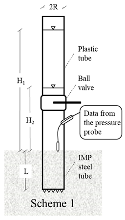
R (0.05 m) and L (0.32 m) are the radius and the submerged length (m) of the tube, respectively, as defined in [17].
H1 and H2 are the water levels (m) in the permeameter cell corresponding to time t1 and t2 (s), respectively.
Pervious (for a total area of 3.11 × 10⁻⁴ m2), with the material inside. Applicability conditions: Ks represents both the horizontal and vertical hydraulic conductivity of the soil Water 12 02286 i002
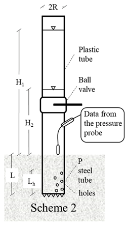
Rmod (0.049 m) and Lmod (0.20 m) are the radius (m) and the submerged length (m), respectively, as calibrated in [18].
H1 and H2 are the water levels (m) in the permeameter cell corresponding to time t1 and t2 (s), respectively.
Lh (0.25 m) is the perforated permeameter length
Table 2. Spatial and temporal variation of the Ks (m day−1) values for the nine piezometers inside the HSTW bed in 2018 [18] and 2019.
Piezometer 20182019Reductions of Ks (%)
Distance from the Inlet (m)KsSDKsSDRelative to Clean Gravel 1In 2019, Relative to 2018
(m day−1) (m day−1) In 2018In 2019
18.53072614420420849886
4176500239750081505677423
725.573105847258134762631
28.54545961225125779995
51710,217293770492146486431
825.553017153770800738129
38.5204557413352212899335
61784497937468517576212
925.56309470728512236863–15
Note: Ks, hydraulic conductivity at saturation; SD standard deviation. 1 Ks = 19,466 m day−1.
Table 3. Spatial and temporal variation of the Ks (m day−1) values along the main transects in 2018 [18] and 2019.
TransectKs (m day−1)Reductions of Ks (%)
Relative to the Clean Gravel 1In 2019, Relative to 2018
20182019In 2018In 2019
1-2-3322166083.596.779.5
4-5-68388650856.966.622.4
7-8-96307610467.668.63.2
Note: Ks hydraulic conductivity at saturation. 1 Ks = 19,466 m day−1.
Table 4. Spatial and temporal variation of the Ks (m day−1) values along the main paths in 2018 [18] and 2019.
PathsKs (m day−1)Reductions of Ks (%)
Relative to Clean Gravel 1In 2019, Relative to 2018
20182019In 2018In 2019
1-4-75627422971.178.324.8
2-5-86687368165.681.145.0
3-6-95601536371.272.44.2
Note: Ks hydraulic conductivity at saturation.1 Ks = 19,466 m day−1.
Table 5. Mean values of the physical–chemical (mg L−1) and bacteriological (CFU 100 mL−1) parameters at the HSTW system inlet and outlet and at the hybrid treatment wetland (TW) outlet during the operation period, April 2016–February 2019.
Mean Values (Standard Deviations) April 2016–February 2019Italian WW Discharge Limits aN Total SamplesN Samples Lower than Limits
HSTW InletHSTW OutletHybrid-TW Outlet
TSS48.6(±42.4)13.3(±9.0)7.0(±5.8)803434
BOD5106.1(±104.9)19.5(±28.4)15.8(±26.6)403736
COD209.4(±203.5)41.3(±54.9)29.8(±47.9)1603736
TN79.5(±26.2)40.6(±20.8)27.6(±11.3)-31
N-NH3+17.6(±21.3)8.1(±13.6)0.7(±1.4)15 b3838
N-NO345.6(±18.5)14.5(±16.2)18.3(±11.4)20 b3719
TP14.6(±7.8)13.5(±9.6)11.2(±7.4)102616
E. coli7.1 × 105(±1.1 × 10⁶)1.3 × 10⁴(±3.7 × 10⁴)6.6 × 101(±1.1 × 10²)5.0 × 1032626
Note: TSS, total suspended solids (mg L−1); BOD5, biological oxygen demand after five days (mg L−1); COD, chemical oxygen demand (mg L−1); PO4, phosphate (mg L−1); TN, total nitrogen (mg L−1); N-NH3, ammonia nitrogen (mg L−1); N-NO3, nitrate nitrogen (mg L−1); E. coli (CFU 100 mL-1). a [33]; b Limit for discharge into surface water bodies.
Table 6. Mean annual values of the water inflow rate (Q) (m3 day−1), total suspended solids rate (TSSLR) (g TSS m−2·day−1), hydraulic loading rate (HLR) (mm day−1), and maximum areal organic loading rate (OLR) (g BOD5 m−2 day−1) of the HSTW unit during the period, 2016–2018. The values are based on the inflow rate through the system.
Mean Annual Values (Standard Deviations)
201620172018
Q23.86(±19.8)31.59(±19.1)32.06(±17.6)
TSSLR4.6(±2.9)4.8(±3.4)6.5(±3.1)
HLR59.6(±19.8)79.0(±19.1)80.1(±17.6)
OLR11.8(±6.9)8.3(±5.4)13.3(±5.6)
Note: Q, water inflow rate; TSSLR, total suspended solids rate; HLR, hydraulic loading rate; OLR, maximum areal organic loading rate.

