Abstract
The application of hydrological models in data-scarce catchments is usually limited by the amount of available data. It is of great significance to investigate the impacts of data quantity and quality on model calibration—as well as to further improve the understanding of the effective estimation of robust model parameters. How to make adequate utilization of external information to identify model parameters of data-scarce catchments is also worthy of further exploration. HBV (Hydrologiska Byråns Vattenbalansavdelning) models was used to simulate streamflow at 15 catchments using input data of different lengths. The transferability of all calibrated model parameters was evaluated for two validation periods. A simultaneous calibration approach was proposed for data-scarce catchment by using data from the catchment with minimal spatial proximity. The results indicate that the transferability of model parameters increases with the increase of data used for calibration. The sensitivity of data length in calibration varies between the study catchments, while flood events show the key impacts on surface runoff parameters. In general, ten-year data are relatively sufficient to obtain robust parameters. For data-scarce catchments, simultaneous calibration with neighboring catchment may yield more reliable parameters than only using the limited data.
1. Introduction
Hydrological models are important tools for rainfall–runoff simulation and flood forecasting around the world [1]. Among different types of models, conceptual models are widely used in the simulation of catchments at different scales due to the relatively low data requirements and simplicity of operation. Parameters of conceptual models normally cannot be estimated directly from catchment characteristics. They usually need to be calibrated based on historical records, such as precipitation, temperature, evapotranspiration and discharge. For many locations—especially for small and medium-sized rivers (the catchment area is between 200 km2 and 3000 km2)—the observations are not available or the observation devices just have been established for a short time [2]. As a result, the application of models is often limited by insufficient data or poor data quality due to instrument failures or low reliability, which can lead to problems in parameter identification. The reliability of models is highly affected by the data sets used for model calibration [3]. How to improve the transferability of model parameters in data-scarce catchments remains a challenge in hydrology [4,5]. It is very important to obtain reliable parameter estimation and accurate flood forecasts in these areas to reduce the loss of life and property [6].
Numerous studies have shown that model parameter estimation is sensitive to the number of data points used in the calibration. Many attempts have been made to investigate the data requirements for good model calibration. Yapo et al. [7] tested the sensitivity of the NWSRFS–SMA conceptual model to different lengths of input data, and they suggested that approximately eight years of data are needed to identify robust parameter estimation. Foglia’s research shows that the parameters of the distributed TOPographic Kinematic APproximation and Integration (TOPKAPI) model are sensitive to the selection of input data [8]. Subsequently, the generalized Cook’s distance approach was introduced by them to have an effective identification of data impacts in hydrological modeling [9]. David et al. [10] evaluated the impacts of data length in a great number of study catchments using a two-stage hybrid framework. High impact was also detected on maximum predicted flows. Li et al. [11] concluded that eight years of data were sufficient to obtain reasonable model parameters, while longer data series did not necessarily yield better results.
The model calibration is also strongly impacted by the quality of observational data. Two data series with the same length of data, but different hydroclimatic conditions often lead to different model parameters. Yapo et al. [7] indicate that the observation records contain relatively wet weather conditions can significantly reduce the uncertainty of model parameters. Wright et al. [12] evaluated the impact of individual data on model simulation based on case-deletion methods and analytical diagnostics in catchments under different climate conditions, the result shows that a single point could change the maximum streamflow prediction by more than 25%. A considerable number of studies have shown that the data series selected for model calibration and validation should be well representative of the various phenomena experienced by the catchment [13,14,15,16]. Continuous series of data covering different weather conditions can effectively reduce the uncertainty of model parameter estimation [11].
However, as mentioned previously, for many small and medium-sized rivers, observations are only available in a short period. For example, through the construction project of early flood warning and forecasting for small and medium-sized rivers in China, a great number of rain gauges and hydrological stations have been built in the past few years [17]. Sudden floods caused by intense rainfall occur frequently in these regions, it is urgent to establish an accurate flood forecasting system to reduce the losses of flood disasters. The main problem at present is that the accumulated data may be insufficient to determine the model parameters, which usually leads to high uncertainties in the parameter estimation. Over the past few decades, a considerable number of studies have been carried out to predict the signatures in ungauged basins by transferring information from gauged catchments based on the idea of hydrological similarity [18,19]. Moreover, a simultaneous calibration for a set of catchments was introduced to find model parameters perform reasonably for all catchments involved in the calibration, which could improve the transferability of model parameters for ungauged basins [20]. This prompts us to consider how to adequately utilize the limited data records of a particular catchment and information from other catchments to obtain accurate runoff forecasts [17]. Therefore, first of all, it is of great importance to evaluate the influences of data quantity and quality in model calibration and parameter identification, to gain more knowledge about how much data and what kind of data sets can be selected to effectively identify robust model parameters. Based on this, further exploration should be focused on how to make full use of the information to obtain parameters with reasonable transfer performance in data-scarce catchments.
This study aims to investigate the impacts of data variation in model calibration, as well as to minimize uncertainty in parameter estimation in data-scarce catchments. Two numeric experiments were conducted on 15 small and medium-sized catchments. In the first experiment, the impacts of data quality and quantity on model calibration were investigated. The HBV (Hydrologiska Byråns Vattenbalansavdelning) model was calibrated for all study catchments using data of different lengths and then the transferability of all calibrated model parameters over two different decades was assessed. In the second study, in order to explore a possible solution for reducing the uncertainty in model parameterization for data-scarce catchments, the simultaneous calibration approach was performed by using information from catchments with minimal spatial proximity.
This study is organized as follows: after the introduction, Section 2 gives a brief description of the study area and hydro-meteorological data. Section 3 explains the methods and the design of two numeric experiments. The results and discussion are presented in Section 4. In Section 5, the summaries and outlook of this research are outlined.
2. Study Area and Hydro-Meteorological Data
The study domain is located in the Mid-Atlantic region of the United States. A total of 15 catchments were used to conduct this study (Figure 1). These catchments are a subset of the dataset used for the model parameter estimation experiment (MOPEX) project [21]. The MOPEX project provides more than 50 years’ continuous daily precipitation, potential evapotranspiration, average air temperature and daily streamflow for vast amounts of catchments. The daily precipitation and air temperature data were supplied by the National Climate Data Center (NCDC, Asheville, NC, USA), while the discharge series was offered by the United States Geological Survey (USGS) gauges. Detailed descriptions of the MOPEX catchments can be found in Duan [21].
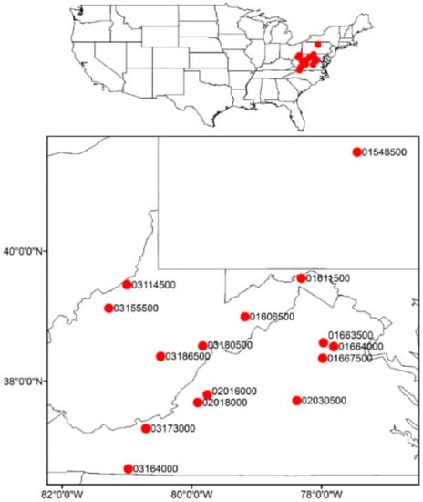
Figure 1.
Location of the selected 15 catchments.
Table 1 lists the catchment properties for the investigate area and Table 2 presents the climate conditions, respectively. It can be seen clearly from tables that the study catchments vary considerably not only in meteorological conditions, but also in catchment characteristics. The smallest catchment has a size of 332 km2, while the biggest one is about 2929 km2. The median size of the catchments is about 1186 km2. The study catchments are impacted by a humid continental climate with relatively warm summers and heavy snowfall in winters. The precipitations are distributed throughout the whole year and show a slight seasonality. The precipitation increases slowly in summer, but the runoff reached the lowest level of the whole year due to the high rate of evapotranspiration. From February to April, the melting of snow leads to a significant increasing in runoff generation. The percentage of snowfall during cold seasons shows an increase from 8.5% in the south region to about 27% at the northeast coast that along with an obvious decline of long-term average temperature from 13.5 °C to 7.2 °C.

Table 1.
Catchment characteristics for the 15 selected model parameter estimation experiment (MOPEX) catchments.
Table 2.
Meteorological conditions for the 15 selected MOPEX catchments.
3. Methodology
3.1. HBV Model
The conceptual HBV model was selected to simulate the rainfall–runoff response for the study catchments. HBV model was originally established at the Swedish Meteorological and Hydrological Institute (SMHI) in the early 70s [22]. Compared with other hydrological models, the HBV model has a relatively simple structure and few parameters. Therefore, it is convenient to run a great number of simulations in a short time. After years of development, HBV has become a multipurpose model with a variety of applications in flood forecasting, water resources management and studies on impacts of climate change around the world [23,24].
The HBV model consists of conceptual routines for snow accumulation and snowmelt, evapotranspiration and soil moisture, runoff generation and runoff concentration. The snow accumulation and snowmelt routine are calculated based on the degree–day method by two parameters: degree–day factor (DD) and threshold temperature for snowmelt (TT). Actual soil moisture is calculated by balancing precipitation and actual evapotranspiration using field capacity (FC) and permanent wilting point (PWP) as parameters. If the soil moisture is greater than PWP, the actual evapotranspiration occurs at a potential rate, otherwise, the evapotranspiration will be limited by the ratio of actual soil moisture to PWP. Runoff generation is calculated by a nonlinear function of precipitation and actual soil moisture with a shape coefficient (Beta). The determined runoff is separated into three different flow components: surface flow, interflow and groundwater, which are represented by two linear reservoirs with corresponding residence time (K0, K1 and K2). The surface flow is restricted by the threshold water level of the upper reservoir (L). The upper and lower reservoirs are connected using a linear percolation rate (KD). Finally, the local runoff is supposed to converge to the outlet through a transformation function based on a triangular weighting parameter (Maxbas). More descriptions of the HBV model can be found in our previous studies [20,25].
The lumped version of the HBV model was selected to simulate the daily scale rainfall–runoff response with areal mean precipitation, potential evapotranspiration and mean air temperature as inputs. As shown in Table 3, a total of 9 parameters were selected to be calibrated using historical data. The initial ranges of model parameters were determined according to literature and pretest results. The robust parameter estimation (ROPE) algorithm was selected for model parameter optimization [26]. The ROPE algorithm is based on the conception of data depth function. The basic idea of this approach is to seek the center points in the multidimensional space constructed from all parameter sets. The Monte-Carlo random sampling method is used to generate a pre-given number of parameter sets based on the possible range of model parameters. The ROPE algorithm is a very efficient calibration method that can result in a pre-given number of parameter sets with fairly good model performance. Considering the nonuniqueness of model parameters, in this study, each calibration results in 10,000 model parameter sets with very similar model performance, but different distributions of the parameter sets. All the calibrated parameter sets are considered to be transferred to other periods. For statistical purposes, the mean model efficiency for the optimal 10,000 parameter sets was used to represent the model performance.
Table 3.
Description and initial range of the HBV model parameters.
3.2. Performance Criteria
The Nash–Sutcliffe coefficient (NS) between the observed and modeled discharge is the most frequently used performance criterion in hydrological modeling [27].
where represents the observed discharge at time t and represents the corresponding modeled discharge, respectively. is the mean observed discharge over the whole calibration period.
Many studies have shown that the selection of the performance criteria has a strong impact on model performance [28]. In this study, according to the available observations, HBV model was simulated on a daily scale. The goal of the model calibration is to capture dynamic behavior and achieve water balance simultaneously. The NS efficiency represents the squared difference between the modeled and observed runoff that pays more attention to high flows than low flows. Therefore, a newly constructed performance criterion by incorporating water balance with NS efficiency was considered in model calibration. Viney et al. [29] suggested to combine NS efficiency and Bias constraints by using the following Equation:
where B denotes the bias value for the total simulated runoff and observed runoff. is a balance factor that specifies the weight to control the severity of the constraint penalty. The value of is 2.5 in this study. This formula takes into account both reasonable water balance and accurate runoff dynamics. The abbreviation NSB (Nash-Sutcliffe and Bias) is used subsequently for this performance measurement.
3.3. Numeric Experiments
In this study, two numeric experiments were designed to evaluate the influences of data quality and quantity on model parameterization, to investigate how much observational data are sufficient or necessary to obtain good model calibration, as well as to explore potential solutions for reducing the uncertainty of model patronization in data-scarce regions.
Numeric Experiment 1 investigates the impacts of data variability in parameter estimation. Daily data from 1950–1989 were split into calibration (1951–1969) and validation (1970–1989) periods. The HBV model was simulated using the ROPE algorithm based on 1, 2, 5 and 10 consecutive years’ data from 1950 to1969. This kind of simulation strategy resulted in 20, 10, 4 and 2 calibration runs for every catchment. To minimize initialization errors caused by uncertainty in the soil moisture state, one-year data before the selected period was taken as a warm-up period. It should be noted that the results of the warm-up period are not considered in the evaluation of the objective function. Two distinct validation periods (1970–1979, 1980–1989) were selected to evaluate the transferability of model parameters. All the calibrated parameter sets were used to simulate the rainfall–runoff for the validation periods. In order to better quantify the transferability of model parameters between different catchments, the HBV models were also calibrated for the period 1970–1979 and 1980–1989 by the ROPE algorithm. The transferability and sensitivity of model parameters are compared based on the validation performances, as well as the distribution of the calibrated parameters.
Numeric Experiment 2 addresses the question of how to incorporate external information into the modeling of data-scarce catchments. We assumed that the target catchment is a sparse catchment with only one-year data, while the neighboring catchment with the minimal spatial distance has long-term observations. The data from neighboring catchment was also considered in model calibration to reduce the uncertainty of parameters. A simultaneous calibration approach was proposed to calibrate the models simultaneously for data-scarce catchment and the neighboring catchment. The goal is to determine robust parameters for data-scarce catchment by using information from the data-rich catchment. The simultaneous calibration method is a multiobjective optimization function, the objective function can be defined as follows:
Here, is the objective function for a given parameter set . and denote the optimal NSB for the neighboring catchment and the data-scarce catchments, respectively. The optimal performance can be represented by the model performance of individual calibration. and denotes the NSB value of parameter set for the neighboring catchment and the data-scarce catchments, respectively. The greater the value of µ is, the more the biggest loss in model performance contributes to the simultaneous calibration. The aim is to maximize the objective function and to find parameter sets perform well for all the catchments involved in calibration. A value of 4 was given for the balance factor to obtain reasonable performance for both catchments.
To find catchments with minimal spatial proximity, the geographic distance between the stream gauges was calculated for pairwise catchments. The ten-year data (1950–1959) of the neighboring catchment was selected to conduct simultaneous calibration with data-scarce catchment using one-year data. Simultaneous calibration was carried out for all data-scarce catchments for the period 1950–1969, which resulted in 20 simulations for every catchment. Afterward, the transferability of the calibrated parameters was also tested for two validation periods (1970–1979, 1980–1989). The validation results were compared with results only using data from data-scarce catchments to explore the benefits of simultaneous calibration.
4. Results and Discussion
4.1. Comparison of Calibration and Validation Performance
First, the model performances of calibration for one-year data and the validation for ten-year data were compared. Figure 2 plots the NSBs of calibration for one-year data and the first validation period (1970–1979). The points are poorly correlated with a correlation coefficient of 0.45. It can be observed that most points lie below the diagonal, indicating that the calibration performances are generally higher than validation values. The result also demonstrates that the parameter set with high calibration NSB may not yield good validation performance. However, a good calibration result is a prerequisite for good validation.
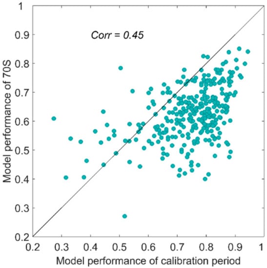
Figure 2.
Comparison of Nash–Sutcliffe and Bias (NSB) for the one-year data based calibration and for the validation of period 1970–1979.
Second, for the two validation periods, the transferred model performances by using parameters calibrated based on one-year data were compared (Figure 3). The NSBs for the two validation periods are similar, with a correlation of 0.8. The correlation values between these two validation periods for the two-year, five-year and ten-year data-based parameter estimation are 0.82, 0.84 and 0.84, respectively. The high correlations imply that the transferability of model parameters is relatively stable, good model performances for the 70s always incorporates perfect simulation for the 80s and vice versa. The difference in model performance between two validation periods increases with the reduction of NSBs, indicating that low-performance simulations are more sensitive to specific periods. This is mainly due to the high uncertainty of model parameters.
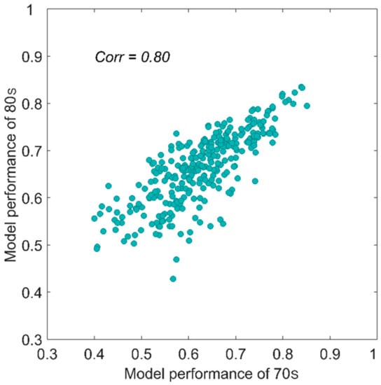
Figure 3.
Comparison of NSBs for the validation period 1970–1979 and 1980–1989 by transferring model parameters from one-year data based model calibration.
4.2. Impact of Data Quality
First, the results of individual calibration for the validation periods were compared. As expected, the model performances show a high positive correlation of 0.93 between 1970–1979 and 1980–1989. The histograms in Figure 4 presents the calibration results for these two periods. Due to measurement errors, the HBV model performs differently for the catchments. For both two validation periods, catchment 15 has the lowest NSB value and catchment 12 shows the highest value, respectively. To have a more equitable comparison between different catchments, we assumed that the individual calibration result is the optimal performance for the validation period. Therefore, all the validation model performances were normalized by the optimal performances. The higher the relative performance means the better the transferability of parameters. A value of 100% means a perfect parameter transfer. The plus signs on the upper part of Figure 4 shows the relative NSBs by transferring model parameters from on one-year data-based calibration (results in 20 validations for each catchment). The result shows that for a specific validation period, the model parameters obtained by short-period data perform differently. Some model parameters can well reproduce the rainfall–runoff response for the study catchments, while some parameters could not obtain reasonable relative NSBs in model validation. It can be seen from the plus signs that, in general, the transferred model performances of 1980–1989 outperformed the results of 1970–1979. For all study catchments, most of the parameters estimated by one-year data can achieve more than 60% relative performances. For catchments 12 and 15, all the parameters calibrated based on one-year data perform well with model performances greater than 80% for both two validation periods.
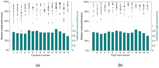
Figure 4.
Model performance by individual calibration and transferred parameters from one-year based calibration:(a) 1970–1979; (b) 1980–1989.
The impacts of data with the same length, but the different quality on model calibration were further discussed. For the calibration based on one-year data, the peak flow and the 10th percentile high flow value were calculated. Figure 5 plots the relative NSBs for 1970–1979 against the peak flow and the 10th percentile high flow of calibration period, respectively. It can be seen clearly from the scatterplots that most of the poor transferred performances (less than 80% relative NSB value) correspond to relatively small peak flows over the calibration period (less than 20 mm). The correlation between model performance and the 10th percentile high flow is not as clear as the peak flow. We can guess that the data sets with low peak flow may not contain as many flood events as the data set with high peak flow. In this case, the calibration process is unable to well capture the dynamic behavior and to reproduce the process of flood events. As a result, the model parameters were underestimated and were not suitable for transfer to other time periods with different climate conditions.
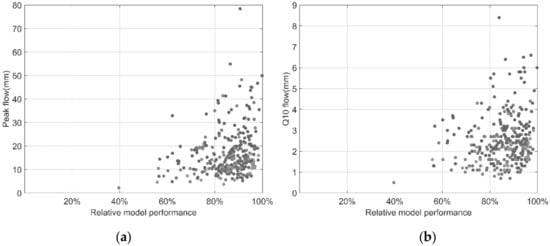
Figure 5.
Comparison of relative NSBs for 1970–1979 and the runoff characteristics during the calibration period. (a) Depth of peak flow; (b) depth of the 10th-percentile high flow.
Furthermore, the correlation between peak flow value and the model parameters was explored. As mentioned previously, we obtained 10,000 parameter sets for each calibration by the ROPE algorithm. Therefore, the mean value and standard deviation of all the optimal parameters were selected to represent the distribution of parameters. The result demonstrates that the peak flow value has a significant influence on the estimation of surface runoff parameters. Figure 6 shows the results for two parameters used for describing surface runoff: threshold water lever (HL) and near surface flow storage constant (K0). The result indicates that for one-year data-based model calibration, the estimation of HL and K0 are highly effected by the peak flow value. A low peak flow implies that the calibration procedure may not provide sufficient information to cope with various climatic conditions, and the hydrological response of the catchment cannot be captured by the model. Therefore, the calibrated parameters are not suitable for transfer to different time periods.
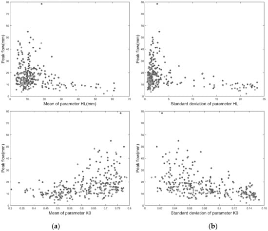
Figure 6.
Comparison of peak flow value and the statistical values of parameters (upper figures) threshold water lever (HL) and (lower figures) residence time (K0). (a) Mean value; (b) standard deviation.
This phenomenon has also been observed in previous studies on the influence of data in model calibration. Yapo et al. [7] found that based on the same length of data, the data set with wet conditions is more sufficient to obtain robust estimates of parameters than the data set with dry conditions. Singh and Bardossy indicated that model calibrated based a small subset of unusual flood events can results in equally good transferability as model parameters calibrated based on the whole observation period [30]. Wright et al. [9] showed that for a two-year based daily model simulation in a semi-arid catchment, removing a peak flow record could strongly affect the estimation of model parameters and the predicting of high flows. The results from this experiment indicate that data quality is of great importance in model calibration. Abundant flood information is important for model parameter identification, which is also a typical challenge for model simulation in data-scarce catchments.
4.3. Impact of Data Quantity
The effects of data quantity on model calibration were investigated by the transferred results of using parameters calibrated based on different lengths of data. Following the design of the first experiment, 20, 10, 4 and 2 validation results were obtained from the calibration based on 1, 2, 5 and 10 continuous years’ data. The mean model performance for each data length category was taken as the transfer result. For a better comparison between different catchments, the results were normalized by the optimal performance for each catchment. Figure 7 shows the mean relative NSBs by transfer parameters that calibrated based on different data lengths for 1970–1979 and 1980–1989, respectively. As expected, for most catchments, the relative NSBs increase significantly with the increase of data length in calibration for both two calibration periods. When the calibration data increases from two to five years, most of the catchments show the greatest increases in model performance. The sensitivity of data lengths in model parameterization varies for the study catchments. For example, the transferability of parameters calibrated based on different lengths of data seems very similar for catchment 9 and 15 in the validation period 1970–1979, while the results are similar for catchment 2, 9, 15 in the validation period 1980–1989. Increasing the quantity of data in model calibration only leads to a slight improvement in validation. However, for catchment 1, the transferred results improve obviously if more years’ data are used for parameter estimation. It can also be found that for some catchments (catchment 2, 3, 9 and 14), the validation NSBs for the period 1970–1979 by transfer parameters from ten-year data-based calibration were slightly smaller than the results based on five-year data. The reason is that the model parameters may be overestimated in the calibration due to the anomalously dry (or wet) climate conditions. There are only 4 and 2 valuation results for the five-year and ten-year data-based calibrations, respectively. Therefore, a single poor transferred performance may have a significant impact on the statistical results. For parameter transfer from ten-year data-based calibration, 11 out of 15 catchments for 1979–1979 and 14 out of 15 catchments for 1980–1989 can obtain more than 90% relative NSBs. The result indicates that ten-year data are sufficient to achieve robust parameter estimations for the study catchments.
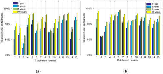
Figure 7.
Relative NSBs by transfer parameters that calibrated based on different lengths of data. (a) 1970–1979; (b) 1980–1989.
The distributions of the model parameters calibrated based on different data lengths were compared. The upper part of Figure 8 shows the typical distribution of the parameter HL and K0 for two catchments, and the lower part of figure shows the corresponding transferred NSBs for 1970–1979, respectively. The distribution range of the selected parameters decreases with the increase of the amount of data, indicating that the uncertainty of parameterization can be reduced if more information is included in the calibration. The model performances improved notably with the increase of data quantity used for calibration. However, for catchment 01611600, when the data length was increased from five to ten years, the relative NSB decreases by 6%. This was mainly due to observational errors and special weather conditions during the calibration. The model was specifically adjusted to the observation period, resulting in the overestimation of model parameters.
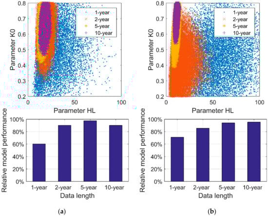
Figure 8.
Distribution of model parameter HL and K0 that calibrated based on (upper) different lengths of data and the (lower) corresponding validation performance. (a) Catchment 01611500; (b) catchment 02016000.
The result of the sensitivity of data length in model calibration is consistent with the general findings of Yapo et al. [7], Anctil et al. [30] and Li et al. [16] where model parameter estimation is strongly affected by the amount of data used in calibration. Based on the large number of experiments that were carried out using different types of models in regions with different climate and underlying conditions, we can conclude that, in general, about eight years of data are required to obtain reliable model parameter estimates. In this study, the result shows that more data series involved in the model calibration usually leads to better transferred model performance. The transferability of model parameters is quite stable while ten-year data were used for model calibration.
In this study, we assumed that the model parameters are constant over time and we did not consider the variation of climatic conditions and catchment characteristics in parameter transfer. However, due to the non-stationary conditions, the model parameters may vary [1,14]. The purpose of modeling is to predict future signatures. Therefore, model parameters should represent the expected climatic conditions and can be transferred to different time periods. Model simulation based on the separation of data series into different climate conditions (e.g., dry and wet periods, warm and cold periods) can help to detect the temporal variations of the model parameters. The transferability of model parameters under non-stationary conditions is worthy of investigation in future work.
4.4. Simultaneous Calibration for Parameterization in Data-Scarce Catchments
As shown before, model parameterization is greatly influenced by the selection of calibration data. Increasing the length of observations shows certain improvements when transferring the parameters to other periods. Furthermore, simultaneous calibration of HBV model was performed for a data-scarce catchment with one-year data and the neighboring catchment with ten-year data (1950–1959) to identify robust parameters for the data-scarce catchment. We treated all study catchments as sparse catchments with only one-year data for calibration. For the data from 1950 to 1969, the simultaneous calibration was carried out for every year separately. It resulted in 20 calibrations and the validation performance was evaluated for the periods 1970–1979 and 1980–1989 as well. The results show that simultaneous calibration always leads to slightly weaker performance than the individual calibration based on one-year data. However, the transferred result for the validation period indicates the robustness of the simultaneous calibration. Taking the validation result of 1970–1979 as an example, the mean NSB of all catchments for individual calibrated parameters is 0.62, while for the simultaneous calibrated parameters the value slightly increases to 0.64. The transferability of simultaneous calibrated parameters was compared with the individual calibrated parameters as shown in Figure 9. It can be seen from the scatterplots that incorporating information from neighboring catchment can provide more reliable parameters for data-scarce catchments. For about 65% of the validation results for 1970–1979 and 64% for 1980–1989, the simultaneous calibrated parameters outperform the individual parameters. Furthermore, approximately 55% of the validation results for both two periods that simultaneous calibration transfer shows better performance than individual transfer. While only about 20% of the individual parameters performed better than simultaneous parameters for both two validation periods. The differences of validated NSBs appears to be greater for data sets with relatively low performances. For data-scarce catchments, if the parameters cannot be effectively identified by itself, using the information from the neighboring catchment is a credible solution to improve the accuracy of prediction. The results suggest that the simultaneous calibration approach offers a possible solution for model parameterization in data-scarce catchments.
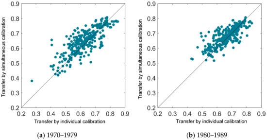
Figure 9.
Comparison of model performances for parameter transfer from individual calibration and simultaneous calibration for periods (a) 1970–1979 and (b) 1980–1989.
It can be found from the scatterplots that a certain number of points lie on the diagonal, indicating that the utilization of additional information does not improve the transferability of the parameters. For about a quarter of the points are located in the lower part of the diagonal, indicating that the parameters of simultaneous calibration lead to weaker model performance than the one by individual calibration. In this study, we assumed that the catchments with spatial proximity are more likely to have similar dynamic behavior. The catchment similarity measurement was not included in the scope of this study. In a simultaneous calibration procedure, only the catchment with the shortest geographical distance was considered. Our previous study of simultaneous calibration for a set of catchments suggests that many catchments share parameters and the selection of catchments for simultaneous calibration is important [20]. This experiment used information from only one neighboring catchment. There are several literatures provide schemes for the identification of catchment similarity based on catchment signatures [19,31,32]. We believe that they could provide some guidance for selecting catchments for simultaneous calibration. In this experiment, only the information from one neighboring catchment was considered, and the simultaneous calibration for a set of similar catchments may be a probable approach to identify parameters data-scarce catchments with robust transferability.
5. Conclusions and Outlook
In this study, we investigated the impacts of data quantity and quality on model calibration and parameter transfer. We also explored the potential solution for model parameterization in data-scarce catchments. Two numeric experiments were conducted on 15 small and medium-sized catchments. The HBV model was used using different lengths of data, the model performances of parameter transfer for two validation periods were evaluated to investigate the impacts of data quality and quantity on model calibration. Meanwhile, the sensitivity of model parameters to high flows were compared. In addition, simultaneous calibration was proposed to incorporate the information from neighboring catchments to improve the parameter estimation in data-scarce catchments. The main findings of this study include:
- (1)
- The model performances of both calibration and validation were greatly affected by the observations used in model calibration. Good calibration result were usually a prerequisite for good validation. Due to different data quality and different climatic conditions, model parameters calibrated based on the same length of data still performed differently;
- (2)
- Flood events during the calibration period had a significant impact on the identification of model parameters, especially for those related to surface runoff generation and concentration. The lack of flood information during the calibration period may have led to the underestimation of model parameters and cause high uncertainty. Abundant flood information was essential to identify model parameters with robust transferability both in space and time;
- (3)
- The transferability of the model parameter increased notably with the increase of the length of data used for model calibration. The sensitivity of data length to parameter estimation varied among the selected catchments. Using ten-year data for calibration, most catchments could obtain more than 90% of the validation model performances, indicating that about ten-year data could achieve reliable parameter estimation for the study catchments;
- (4)
- For model parameter estimation in the data-scarce catchment, the result showed that simultaneous calibration with neighboring catchment could lead to more reliable parameter estimations than only using the limited data. The model parameters could be identified by information from other catchments with a high degree of similarity. The simultaneous calibration approach offered a potential approach for model parameterization in data-scarce catchments.
This research further demonstrates that model parameter estimation is a complex process. Although we know that the model parameterization is highly dependent on the observations used for calibration, it is still difficult to quantify the impact due to the varying sensitivities of data in different catchments. The catchment similarity measurement was not explicitly treated in this research, and more studies are required to further investigate the simultaneous calibration approach for catchments with a similar hydrological response. This can further enhance the transferability of model parameters in data-scarce regions. Currently, all the models were simulated on a daily scale. For small and medium-sized catchments, the floods often converge to the outlet very quickly with short leading times. Therefore, the hourly response of the catchments also deserves to be explored in future work.
Author Contributions
Conceptualization, A.B. and Y.H.; data curation, Y.H.; formal analysis, A.B. and Y.H.; funding acquisition, Y.H.; methodology, A.B. and Y.H.; project administration, Y.H.; resources, A.B.; software, A.B. and Y.H.; supervision, A.B.; validation, Y.H.; visualization, Y.H.; writing—original draft, Y.H.; writing—review & editing, Y.H. and A.B. All authors have read and agreed to the published version of the manuscript.
Funding
This research was funded by the National Key R&D Program of China (Grant No. 2018YFC1508102), the National Natural Science Foundation of China (Grant No. 51909059), the Fundamental Research Funds for the Central Universities (Grant No. B200202036), the Natural Science Foundation of Jiangsu Province (Grant No. BK20190492), the Chinese Postdoctoral Science Foundation (Grant No. 2017M621614) and the Postdoctoral Research Supporting Program of Jiangsu Province (Grant No. 2018K128C).
Conflicts of Interest
The authors declare no conflict of interest.
References
- Minville, M.; Cartier, D.; Guay, C.; Leclaire, L.A.; Audet, C.; Le Digabel, S.; Merleau, J. Improving process representation in conceptual hydrological model calibration using climate simulations. Water Resour. Res. 2014, 50, 5044–5073. [Google Scholar] [CrossRef]
- Yao, C.; Zhang, K.; Yu, Z.; Li, Z.; Li, Q. Improving the flood prediction capability of the Xinanjiang model in ungauged nested catchments by coupling it with the geomorphologic instantaneous unit hydrograph. J. Hydrol. 2014, 517, 1035–1048. [Google Scholar] [CrossRef]
- Bardossy, A. Calibration of hydrological model parameters for ungauged catchments. Hydrol. Earth Syst. Sci. 2007, 11, 703–710. [Google Scholar] [CrossRef]
- Ren, H.Y.; Hou, Z.S.; Huang, M.Y.; Bao, J.; Sun, Y.; Tesfa, T.; Leung, L.R. Classification of hydrological parameter sensitivity and evaluation of parameter transferability across 431 US MOPEX basins. J. Hydrol. 2016, 536, 92–108. [Google Scholar] [CrossRef]
- Li, C.Z.; Zhang, L.; Wang, H.; Zhang, Y.Q.; Yu, F.L.; Yan, D.H. The transferability of hydrological models under nonstationary climatic conditions. Hydrol. Earth Syst. Sci. 2012, 16, 1239–1254. [Google Scholar] [CrossRef]
- Liu, Z.Y.; Martina, M.L.; Todini, E. Flood forecasting using a fully distributed model: Application of the TOPKAPI model to the Upper Xixian catchment. Hydrol. Earth Syst. Sci. 2005, 9, 347–364. [Google Scholar] [CrossRef]
- Yapo, P.O.; Gupta, H.V.; Sorooshian, S. Automatic calibration of conceptual rainfall-runoff models: Sensitivity to calibration data. J. Hydrol. 1996, 181, 23–48. [Google Scholar] [CrossRef]
- Foglia, L.; Hill, M.C.; Mehl, S.W.; Burlando, P. Sensitivity analysis, calibration, and testing of a distributed hydrological model using error-based weighting and one objective function. Water Resour. Res. 2009, 45, W06427. [Google Scholar] [CrossRef]
- Wright, D.P.; Thyer, M.; Westra, S. Influential point detection diagnostics in the context of hydrological model calibration. J. Hydrol. 2015, 527, 1161–1172. [Google Scholar] [CrossRef]
- Wright, D.P.; Thyer, M.; Westra, S.; Renard, B.; McInerney, D. A generalised approach for identifying influential data in hydrological modelling. Environ. Model. Softw. 2019, 111, 231–247. [Google Scholar] [CrossRef]
- Wright, D.P.; Thyer, M.; Westra, S.; McInerney, D. A hybrid framework for quantifying the influence of data in hydrological model calibration. J. Hydrol. 2018, 561, 211–222. [Google Scholar] [CrossRef]
- Bardossy, A.; Das, T. Influence of rainfall observation network on model calibration and application. Hydrol. Earth Syst. Sci. 2008, 12, 77–89. [Google Scholar] [CrossRef]
- Beven, K.; Binley, A. The Future of Distributed Models—Model Calibration and Uncertainty Prediction. Hydrol. Process. 2010, 6, 279–298. [Google Scholar] [CrossRef]
- Coron, L.; Andréassian, V.; Perrin, C.; Lerat, J.; Vaze, J.; Bourqui, M.; Hendrickx, F. Crash testing hydrological models in contrasted climate conditions: An experiment on 216 Australian catchments. Water Resour. Res. 2012, 48, 213–223. [Google Scholar] [CrossRef]
- Daggupati, P.; Yen, H.; White, M.J.; Srinivasan, R.; Arnold, J.G.; Keitzer, C.S.; Sowa, S.P. Impact of model development, calibration and validation decisions on hydrological simulations in West Lake Erie Basin. Hydrol. Process. 2016, 29, 5307–5320. [Google Scholar] [CrossRef]
- Chuan-Zhe, L.I.; Wang, H.; Liu, J.; Yan, D.H.; Yu, F.L.; Zhang, L. Effect of calibration data series length on performance and optimal parameters of hydrological model. Water Sci. Eng. 2010, 3, 378–393. [Google Scholar]
- Shi, W.; Li, L.; Xia, J.; Gippel, C.J. A hydrological model modified for application to flood forecasting in medium and small-scale catchments. Arab. J. Geosci. 2016, 9, 296. [Google Scholar] [CrossRef]
- Hrachowitz, M.; Savenije, H.H.G.; Blöschl, G.; Mcdonnell, J.J.; Sivapalan, M.; Pomeroy, J.W.; Arheimer, B.; Blume, T.; Clark, M.P.; Ehret, U. A decade of Predictions in Ungauged Basins (PUB)—A review. Hydrol. Sci. J. 2013, 58, 1198–1255. [Google Scholar] [CrossRef]
- Wagener, T.; Sivapalan, M.; Troch, P.; Woods, R. Catchment Classification and Hydrologic Similarity. Geogr. Compass 2007, 1, 901–931. [Google Scholar] [CrossRef]
- Bardossy, A.; Huang, Y.C.; Wagener, T. Simultaneous calibration of hydrological models in geographical space. Hydrol. Earth Syst. Sci. 2016, 20, 2913–2928. [Google Scholar] [CrossRef]
- Duan, Q.; Schaake, J.; Andreassian, V.; Franks, S.; Goteti, G.; Gupta, H.V.; Gusev, Y.M.; Habets, F.; Hall, A.; Hay, L.; et al. Model Parameter Estimation Experiment (MOPEX): An overview of science strategy and major results from the second and third workshops. J. Hydrol. 2006, 320, 3–17. [Google Scholar] [CrossRef]
- Bergström, S. Development and Application of a Conceptual Runoff Model for Scandinavian Catchments; Smhi Reports on Hydrology; SMHI: Norrköping, Sweden, 1976. [Google Scholar]
- Kobold, M.; Brilly, M. The use of HBV model for flash flood forecasting. Nat. Hazards Earth Syst. Sci. 2006, 6, 407–417. [Google Scholar] [CrossRef]
- Lindström, G.; Johansson, B.; Persson, M.; Gardelin, M.; Bergström, S. Development and test of the distributed HBV-96 hydrological model. J. Hydrol. 1997, 201, 272–288. [Google Scholar] [CrossRef]
- Huang, Y.C.; Bardossy, A.; Zhang, K. Sensitivity of hydrological models to temporal and spatial resolutions of rainfall data. Hydrol. Earth Syst. Sci. 2019, 23, 2647–2663. [Google Scholar] [CrossRef]
- Bárdossy, A.; Singh, S.K. Robust estimation of hydrological model parameters. Hydrol. Earth Syst. Sci. 2008, 12, 1273–1283. [Google Scholar] [CrossRef]
- Nash, J.E.; Sutcliffe, J.V. River flow forecasting through conceptual models part I—A discussion of principles. J. Hydrol. 1970, 10, 282–290. [Google Scholar] [CrossRef]
- Yapo, P.O.; Gupta, H.V.; Sorooshian, S. Multi-objective global optimization for hydrologic models. J. Hydrol. 1998, 204, 83–97. [Google Scholar] [CrossRef]
- Viney, N.R.; Perraud, J.; Vaze, J.; Chiew, F.H.S.; Post, D.A.; Yang, A. The Usefulness of Bias Constraints in Model Calibration for Regionalisation to Ungauged Catchments; University Western Australia: Nedlands, Australia, 2009; pp. 3421–3427. [Google Scholar]
- Anctil, F.; Perrin, C.; Andreassian, V. Impact of the length of observed records on the performance of ANN and of conceptual parsimonious rainfall-runoff forecasting models. Environ. Model. Softw. 2004, 19, 357–368. [Google Scholar] [CrossRef]
- Ali, G.; Tetzlaff, D.; Soulsby, C.; McDonnell, J.J.; Capell, R. A comparison of similarity indices for catchment classification using a cross-regional dataset. Adv. Water Resour. 2012, 40, 11–22. [Google Scholar] [CrossRef]
- Sawicz, K.; Wagener, T.; Sivapalan, M.; Troch, P.A.; Carrillo, G. Catchment classification: Empirical analysis of hydrologic similarity based on catchment function in the eastern USA. Hydrol. Earth Syst. Sci. 2011, 15, 2895–2911. [Google Scholar] [CrossRef]


© 2020 by the authors. Licensee MDPI, Basel, Switzerland. This article is an open access article distributed under the terms and conditions of the Creative Commons Attribution (CC BY) license (http://creativecommons.org/licenses/by/4.0/).