Actual Evapotranspiration and Biomass of Maize from a Red–Green-Near-Infrared (RGNIR) Sensor on Board an Unmanned Aerial Vehicle (UAV)

 , , , , and
Abstract
:1. Introduction
2. Material and Methods
2.1. Study Area
2.2. Crop Planting and Management
2.3. Data Acquisition
2.3.1. Field Data
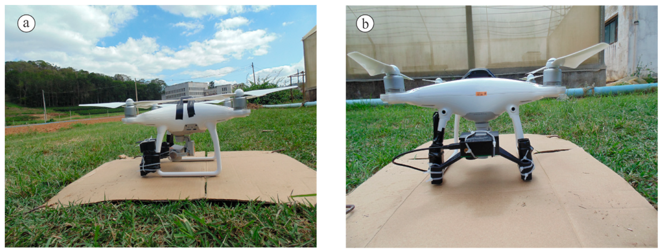
2.3.2. Aerial Data
2.4. Data Processing
2.4.1. Geometric Correction
2.4.2. Conversion from Digital Numbers to Physical Values
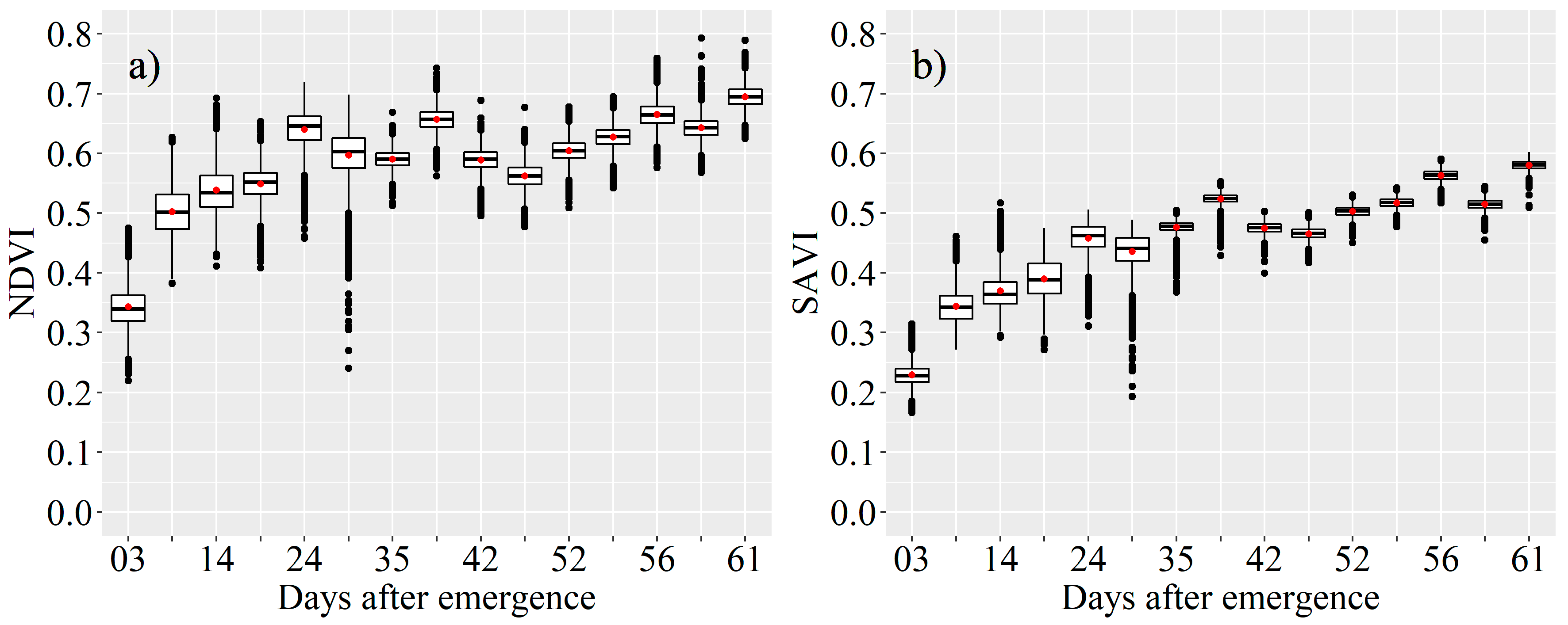
2.4.3. Vegetation Indices (VI)
2.4.4. Actual Crop Evapotranspiration from VI
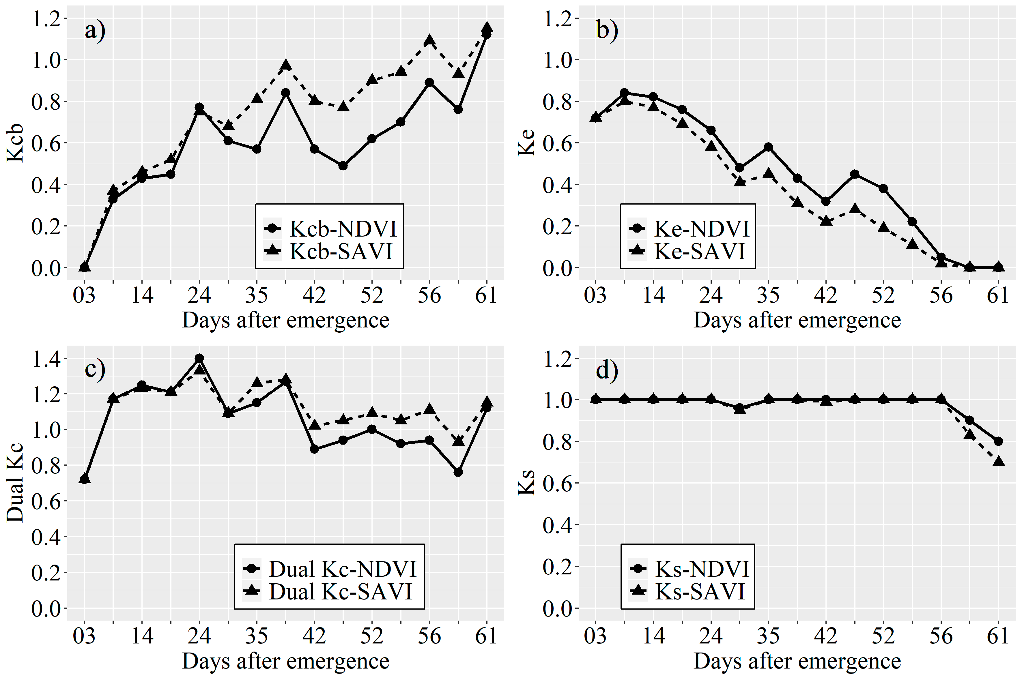
Kcb Estimated by the VI
Evaporation Coefficient (Ke)
Stress Coefficient (Ks)
2.4.5. Estimation of Aboveground Dry Biomass
2.5. Validation of Estimated Aboveground Dry Biomass
3. Results and Discussion
3.1. Kcb Derived from the VIs
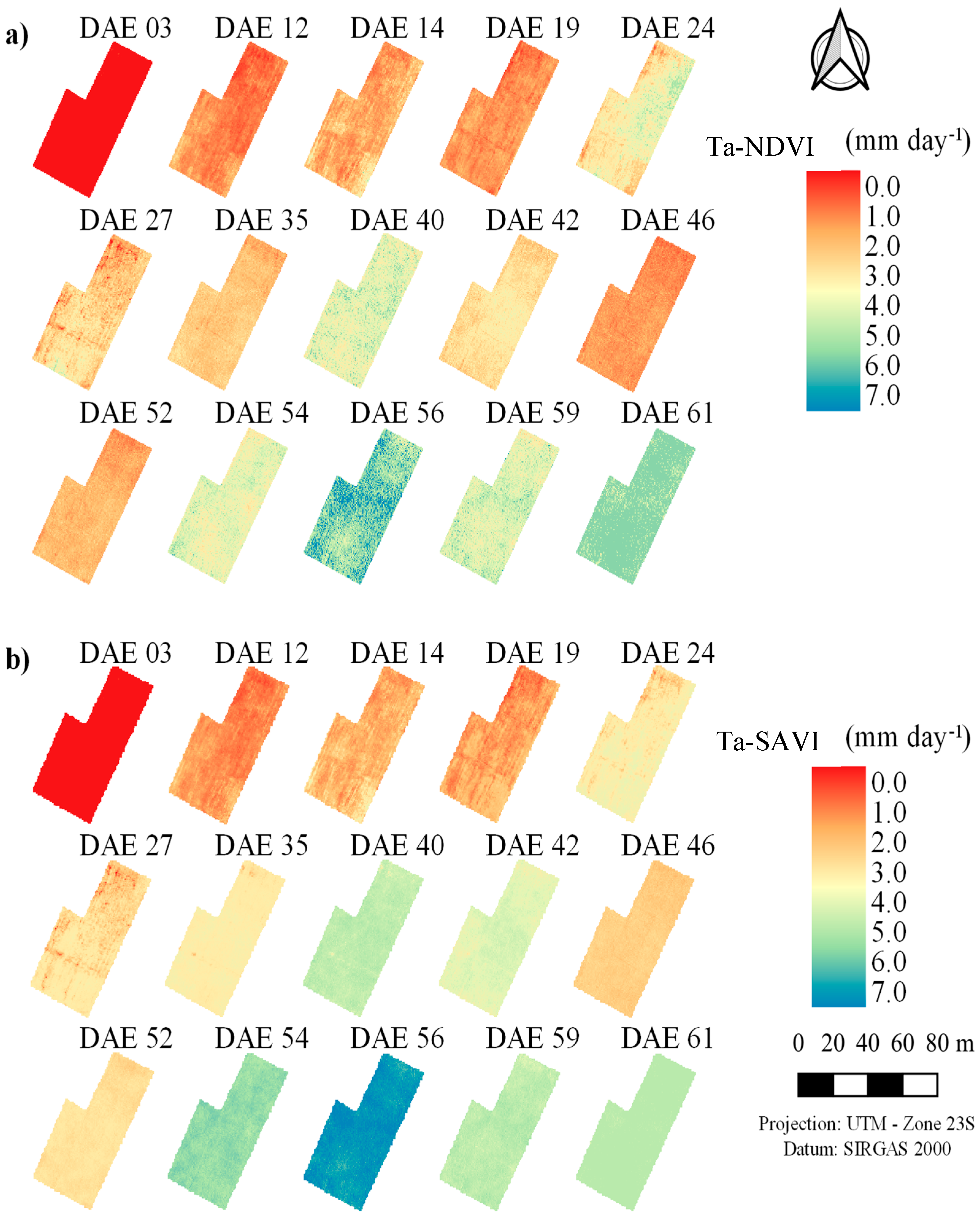
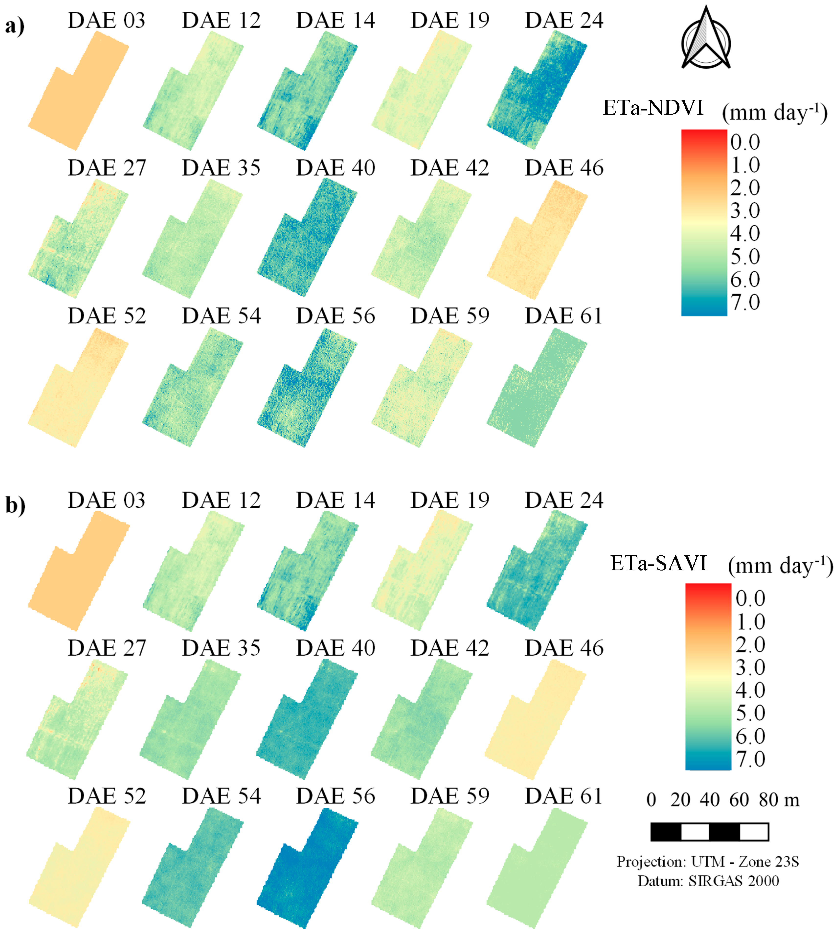
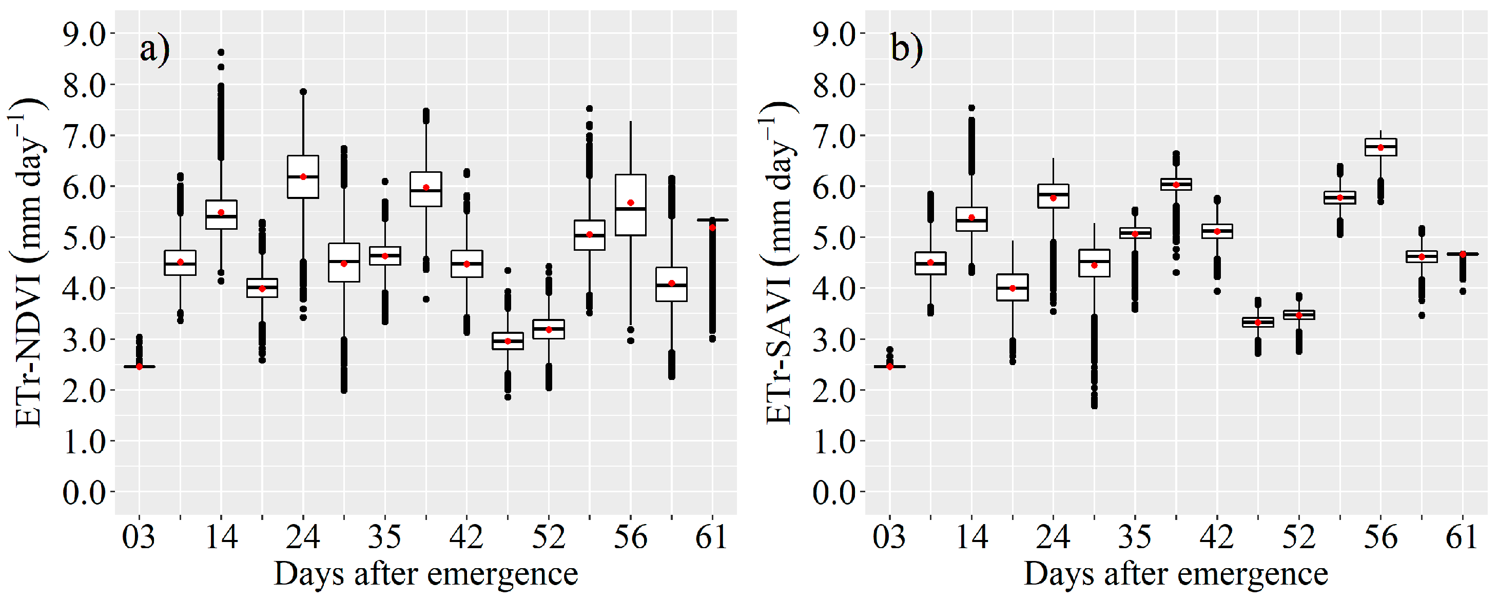
3.2. Actual Transpiration and Evapotranspiration of the Maize Crop
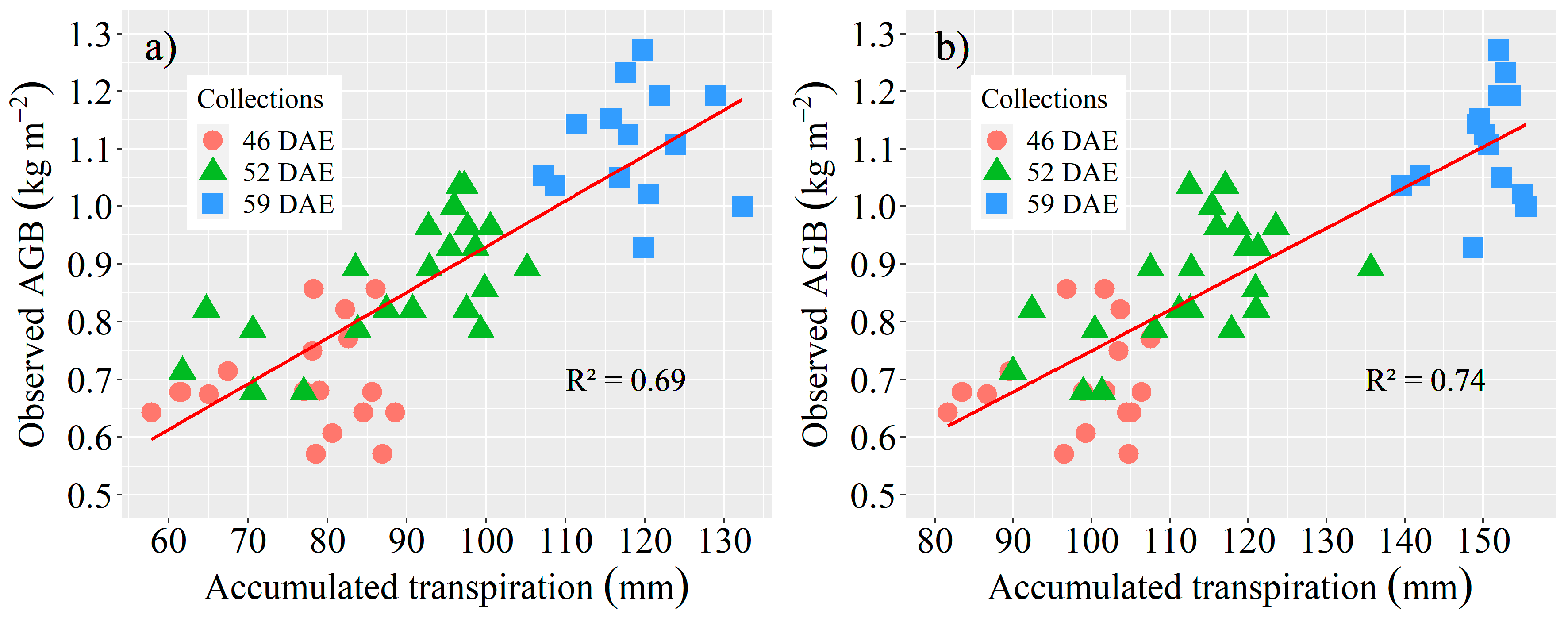
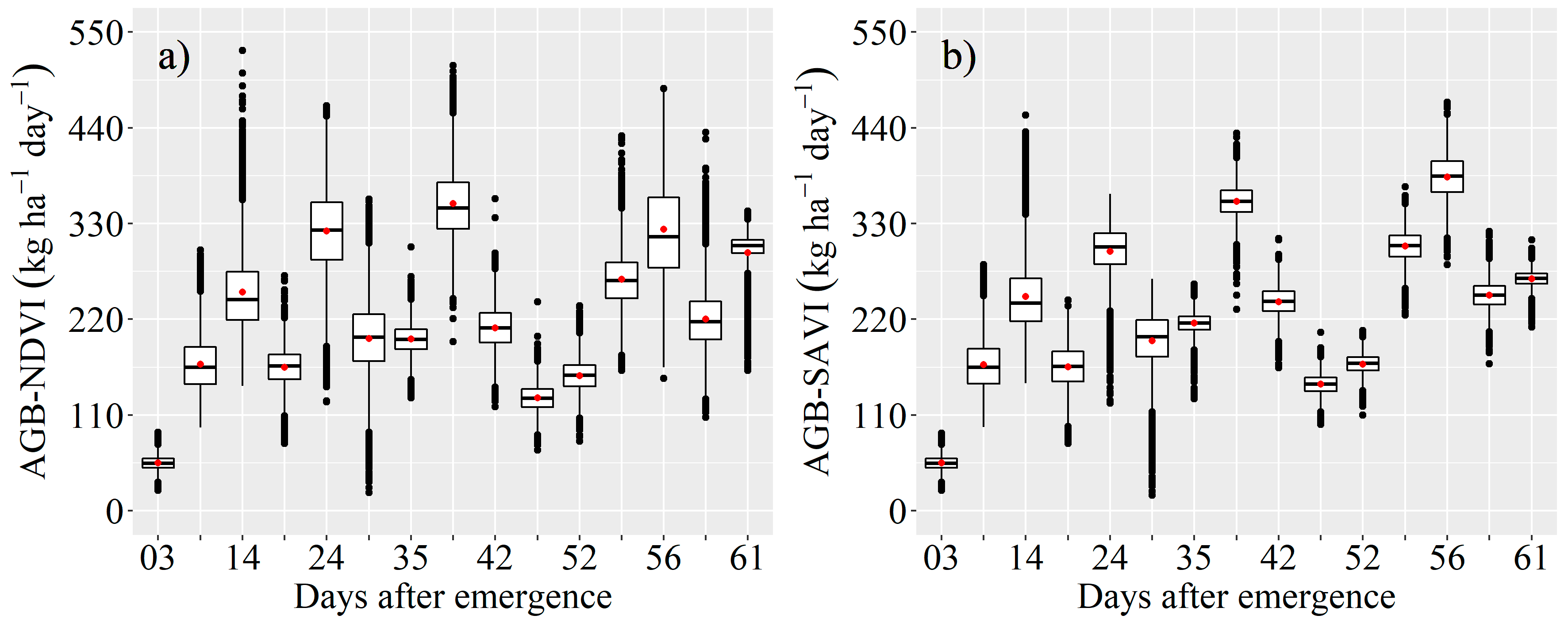
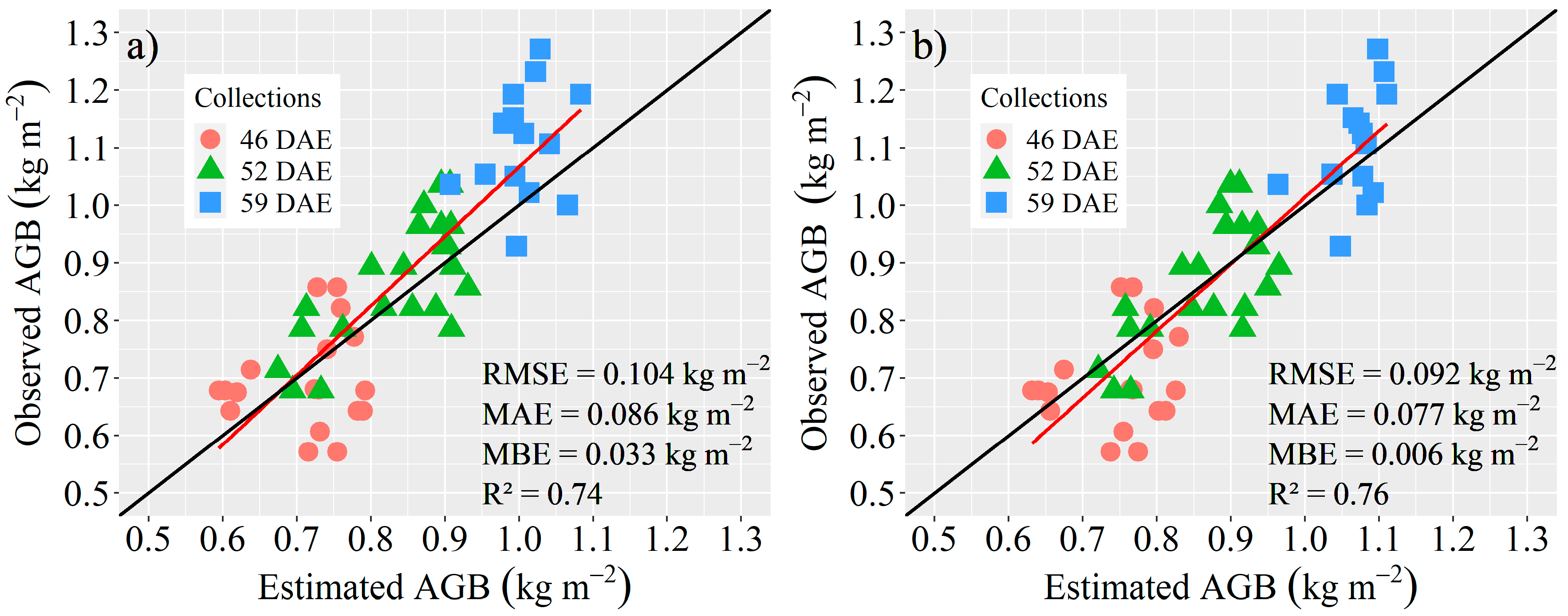
3.3. Estimation of AGB
4. Conclusions
Author Contributions
Funding
Conflicts of Interest
References
- Zheng, H.; Ying, H.; Yin, Y.; Wang, Y.; He, G.; Bian, Q.; Cui, Z.; Yang, Q. Irrigation leads to greater maize yield at higher water productivity and lower environmental costs: A global meta-analysis. Agric. Ecosyst. Environ. 2019, 273, 62–69. [Google Scholar] [CrossRef]
- Tilman, D.; Balzer, C.; Hill, J.; Befort, B.L. Global food demand and the sustainable intensification of agriculture. Proc. Natl. Acad. Sci. USA 2011, 108, 20260–20264. [Google Scholar] [CrossRef] [PubMed] [Green Version]
- UNESCO. Water in a Changing World: The United Nations World Water Development Report 3. 2009. Available online: http://www.unesco.org/new/fileadmin/MULTIMEDIA/HQ/SC/pdf/WWDR3_Facts_and_Figures.pdf (accessed on 19 July 2020).
- Mulla, D.J. Twenty five years of remote sensing in precision agriculture: Key advances and remaining knowledge gaps. Biosyst. Eng. 2013, 114, 358–371. [Google Scholar] [CrossRef]
- Hunt, E.R.; Daughtry, C.S.T. What good are unmanned aircraft systems for agricultural remote sensing and precision agriculture? Int. J. Remote Sens. 2018, 39, 5345–5376. [Google Scholar] [CrossRef] [Green Version]
- Tunca, E.; Köksal, E.S.; Çetin, S.; Ekiz, N.M.; Balde, H. Yield and leaf area index estimations for sunflower plants using unmanned aerial vehicle images. Environ. Monit. Assess. 2018, 190, 682. [Google Scholar] [CrossRef]
- Manfreda, S.; McCabe, M.F.; Miller, P.E.; Lucas, R.; Madrigal, V.P.; Mallinis, G.; Dor, E.B.; Helman, D.; Estes, L.; Ciraolo, G.; et al. On the use of unmanned aerial systems for environmental monitoring. Remote Sens. 2018, 10, 641. [Google Scholar] [CrossRef] [Green Version]
- Maes, W.H.; Steppe, K. Perspectives for remote sensing with unmanned aerial vehicles in precision agriculture. Trends Plant Sci. 2019, 24, 152–164. [Google Scholar] [CrossRef]
- Rabatel, G.; Gorretta, N.; Labbé, S. Getting simultaneous red and near-infrared band data from a single digital camera for plant monitoring applications: Theoretical and practical study. Biosyst. Eng. 2014, 117, 2–14. [Google Scholar] [CrossRef] [Green Version]
- Gowravaram, S.; Tian, P.; Flanagan, H.; Goyer, J.; Chao, H. UAS-based multispectral remote sensing and ndvi calculation for post disaster assessment. ICUAS 2018 2018, 684–691. [Google Scholar] [CrossRef]
- Nijland, W.; de Jong, R.; de Jong, S.M.; Wulder, M.A.; Bater, C.W.; Coops, N.C. Monitoring plant condition and phenology using infrared sensitive consumer grade digital cameras. Agric. Meteorol. 2014, 184, 98–106. [Google Scholar] [CrossRef] [Green Version]
- Bausch, W.C.; Neale, C.M.U. Crop coefficients derived from reflected canopy radiation—A concept. Trans. ASAE 1987, 30, 703–709. [Google Scholar] [CrossRef]
- Er-Raki, S.; Chehbouni, A.; Guemouria, N.; Duchemin, B.; Ezzahar, J.; Hadria, R. Combining FAO-56 model and ground-based remote sensing to estimate water consumptions of wheat crops in a semi-arid region. Agric. Water Manag. 2007, 87, 41–54. [Google Scholar] [CrossRef] [Green Version]
- González-Dugo, M.P.; Mateos, L. Spectral vegetation indices for benchmarking water productivity of irrigated cotton and sugarbeet crops. Agric. Water Manag. 2008, 95, 48–58. [Google Scholar] [CrossRef]
- Campos, I.; Neale, C.M.U.; Arkebauer, T.J.; Suyker, A.E.; Gonçalves, I.Z. Water productivity and crop yield: A simplified remote sensing driven operational approach. Agric. Meteorol. 2018, 249, 501–511. [Google Scholar] [CrossRef]
- Allen, R.G.; Pereira, L.S.; Raes, D.; Smith, M. Crop Evapotranspiration—Guidelines for Computing Crop Water Requirements—FAO Irrigation and Drainage Paper 56, 9th ed.; Food and Agriculture Organization of the United Nations: Rome, Italy, 1998; ISBN 92-5-104219-5. [Google Scholar]
- Li, X.; Kang, S.; Zhang, X.; Li, F.; Lu, H. Deficit irrigation provokes more pronounced responses of maize photosynthesis and water productivity to elevated CO2. Agric. Water Manag. 2018, 195, 71–83. [Google Scholar] [CrossRef]
- Grosso, C.; Manoli, G.; Martello, M.; Chemin, Y.H.; Pons, D.H.; Teatini, P.; Piccoli, I.; Morari, F. Mapping maize evapotranspiration at field scale using SEBAL: A comparison with the FAO method and soil-plant model simulations. Remote. Sens. 2018, 10, 1452. [Google Scholar] [CrossRef] [Green Version]
- Bastiaanssen, W.G.M.; Ali, S. A new crop yield forecasting model based on satellite measurements applied across the Indus Basin, Pakistan. Agric. Ecosyst. Environ. 2003, 94, 321–340. [Google Scholar] [CrossRef]
- Liu, J.; Pattey, E.; Miller, J.R.; McNairn, H.; Smith, A.; Hu, B. Estimating crop stresses, aboveground dry biomass and yield of corn using multi-temporal optical data combined with a radiation use efficiency model. Remote Sens. Environ. 2010, 114, 1167–1177. [Google Scholar] [CrossRef]
- Zwart, S.J.; Bastiaanssen, W.G.M. SEBAL for detecting spatial variation of water productivity and scope for improvement in eight irrigated wheat systems. Agric. Water Manag. 2007, 89, 287–296. [Google Scholar] [CrossRef]
- Wagle, P.; Bhattarai, N.; Gowda, P.H.; Kakani, V.G. Performance of five surface energy balance models for estimating daily evapotranspiration in high biomass sorghum. ISPRS J. Photogramm. Remote Sens. 2017, 128, 192–203. [Google Scholar] [CrossRef] [Green Version]
- Alvares, C.A.; Stape, J.L.; Sentelhas, P.C.; De Moraes Gonçalves, J.L.; Sparovek, G. Köppen’s climate classification map for Brazil. Meteorol. Z. 2013, 22, 711–728. [Google Scholar] [CrossRef]
- INMET. Normais Climatológicas (1961–2018). 2019. Available online: http://www.inmet.gov.br/portal/index.php?r=clima/normaisClimatologicas (accessed on 5 March 2020).
- Santos, H.; Jacomine, P.; Anjos, L.; Oliveira, V.; Lumbreras, J.; Coelho, M.; Almeida, J.; Cunha, T.; Oliveira, J. Embrapa: Sistema Brasileiro de Classificação de Solos, 5th ed.; Embrapa, Ed.: Brasília-DF, Brasil, 2018; ISBN 9788570358004. Available online: https://www.embrapa.br/solos/busca-de-publicacoes/-/publicacao/1094003/sistema-brasileiro-de-classificacao-de-solos (accessed on 10 June 2019).
- Yang, H.; Lee, Y.; Jeon, S.Y.; Lee, D. Multi-rotor drone tutorial: Systems, mechanics, control and state estimation. Intell. Serv. Robot. 2017, 10, 79–93. [Google Scholar] [CrossRef]
- Mapir. Available online: https://www.mapir.camera/products/survey3w-camera-red-green-nir-rgn-ndvi (accessed on 16 January 2019).
- Qgis; Version 2.18; Software For Geographic Information System; Open Source Geospatial Foundation: Chicago, IL, USA, 2016.
- Rouse, R.W.H.; Haas, J.A.W.; Deering, D.W. Monitoring vegetation systems in the great plains with ERTS. Third Earth Resour. Technol. Satell. Symp. Tech. Present. Nasa Sp-351 1974, I, 309–317. [Google Scholar]
- Huete, A. A soil-adjusted vegetation index (SAVI). Remote Sens. Environ. 1988, 25, 295–309. [Google Scholar] [CrossRef]
- García, P.; Pérez, E. Mapping of soil sealing by vegetation indexes and built-up index: A case study in Madrid (In Spain). Geoderma 2016, 268, 100–107. [Google Scholar] [CrossRef]
- Gilabert, M.A.; González-Piqueras, J.; García-Haro, F.J.; Meliá, J. A generalized soil-adjusted vegetation index. Remote Sens. Environ. 2002, 82, 303–310. [Google Scholar] [CrossRef]
- Zhang, L.; Niu, Y.; Zhang, H.; Han, W.; Li, G.; Tang, J.; Peng, X. Maize canopy temperature extracted from UAV thermal and RGB imagery and its application in water stress monitoring. Front. Plant Sci. 2019, 10, 1–18. [Google Scholar] [CrossRef]
- Taiz, L.; Zeiger, E.; max Moller, I.; Murphy, A. Plant Physiology & Development; Sinauer Associates Inc.: Sunderland, MA, USA, 2015; ISBN 9781605352558. [Google Scholar]
- Choudhury, B.J.; Ahmed, N.U.; Idso, S.B.; Reginato, R.J.; Daughtry, C.S.T. Relations between evaporation coefficients and vegetation indices studied by model simulations. Remote Sens. Environ. 1994, 50, 1–17. [Google Scholar] [CrossRef]
- Monteith, J.L. Solar radiation and productivity in tropical ecosystems. J. Appl. Ecol. 1972, 9, 747. [Google Scholar] [CrossRef] [Green Version]
- Coaguila, D.N.; Hernandez, F.B.T.; de Teixeira, A.H.C.; Franco, R.A.M.; Leivas, J.F. Water productivity using SAFER—Simple algorithm for evapotranspiration retrieving in watershed. Rev. Bras. Eng. Agrícol. E Ambient. 2017, 21, 524–529. [Google Scholar] [CrossRef] [Green Version]
- Teixeira, A.D.; de Miranda, F.R.; Leivas, J.F.; Pacheco, E.P.; Garçon, E.A.M. Water productivity assessments for dwarf coconut by using Landsat 8 images and agrometeorological data. ISPRS J. Photogramm. Remote Sens. 2019, 155, 150–158. [Google Scholar] [CrossRef]
- Hatfield, J.L.; Asrar, G.; Kanemasu, E.T. Intercepted photosynthetically active radiation estimated by spectral reflectance. Remote Sens. Environ. 1984, 14, 65–75. [Google Scholar] [CrossRef]
- Asrar, G.; Myneni, R.B.; Choudhury, B.J. Spatial heterogeneity in vegetation canopies and remote sensing of absorbed photosynthetically active radiation: A modeling study. Remote Sens. Environ. 1992, 41, 85–103. [Google Scholar] [CrossRef]
- Moran, M.S.; Maas, S.J.; Pinter, P.J. Combining remote sensing and modeling for estimating surface evaporation and biomass production. Remote Sens. Rev. 1995, 12, 335–353. [Google Scholar] [CrossRef]
- Toureiro, C.; Serralheiro, R.; Shahidian, S.; Sousa, A. Irrigation management with remote sensing: Evaluating irrigation requirement for maize under Mediterranean climate condition. Agric. Water Manag. 2017, 184, 211–220. [Google Scholar] [CrossRef]
- Taghvaeian, S.; Chávez, J.L.; Hansen, N.C. Infrared thermometry to estimate crop water stress index and water use of irrigated maize in northeastern Colorado. Remote. Sens. 2012, 4, 3619–3637. [Google Scholar] [CrossRef] [Green Version]
- Duchemin, B.; Hadria, R.; Erraki, S.; Boulet, G.; Maisongrande, P.; Chehbouni, A.; Escadafal, R.; Ezzahar, J.; Hoedjes, J.C.B.; Kharrou, M.H.; et al. Monitoring wheat phenology and irrigation in Central Morocco: On the use of relationships between evapotranspiration, crops coefficients, leaf area index and remotely-sensed vegetation indices. Agric. Water Manag. 2006, 79, 1–27. [Google Scholar] [CrossRef]
- Rosa, R.D.; Ramos, T.B.; Pereira, L.S. The dual Kc approach to assess maize and sweet sorghum transpiration and soil evaporation under saline conditions: Application of the SIMDualKc model. Agric. Water Manag. 2016, 177, 77–94. [Google Scholar] [CrossRef]
- Nascentes, R.F.; Carbonari, C.A.; Simões, P.S.; Brunelli, M.C.; Velini, D.; Duke, S.O. Low doses of glyphosate enhance growth, CO 2 assimilation, stomatal conductance and transpiration in sugarcane and eucalyptus. Pest Manag. Sci. 2017, 74, 1197–1205. [Google Scholar] [CrossRef]
- Kim, T.-H.; Böhmer, M.; Hu, H.; Nishimura, N.; Schroeder, J.I. Guard cell signal transduction network: Advances in understanding abscisic Acid, CO2, and Ca2+ Signaling. Annu. Rev. Plant Biol. 2010, 61, 561–591. [Google Scholar] [CrossRef] [Green Version]
- Kang, S.; Zhang, F.; Hu, X.; Zhang, J. Benefits of CO2 enrichment on crop plants are modified by soil water status. Plant Soil 2002, 238, 69–77. [Google Scholar] [CrossRef]
- Driscoll, S.P.; Prins, A.; Olmos, E.; Kunert, K.J.; Foyer, C.H. Specification of adaxial and abaxial stomata, epidermal structure and photosynthesis to CO2 enrichment in maize leaves. J. Exp. Bot. 2006, 57, 381–390. [Google Scholar] [CrossRef] [PubMed] [Green Version]
- Campos, I.; González-Gómez, L.; Villodre, J.; González-Piqueras, J.; Suyker, A.E.; Calera, A. Remote sensing-based crop biomass with water or light-driven crop growth models in wheat commercial fields. Field Crop. Res. 2018, 216, 175–188. [Google Scholar] [CrossRef]
- Twohey, R.J.; Roberts, L.M.; Studer, A.J. Leaf stable carbon isotope composition reflects transpiration efficiency in Zea mays. Plant J. 2019, 97, 475–484. [Google Scholar] [CrossRef] [PubMed] [Green Version]
- Fandiño, M.; Cancela, J.J.; Rey, B.J.; Martínez, E.M.; Rosa, R.G.; Pereira, L.S. Using the dual-K c approach to model evapotranspiration of Albariño vineyards (Vitis vinifera L. cv. Albariño) with consideration of active ground cover. Agric. Water Manag. 2012, 112, 75–87. [Google Scholar] [CrossRef]
- Yang, Y.; Xu, W.; Hou, P.; Liu, G.; Liu, W.; Wang, Y.; Zhao, R.; Ming, B.; Xie, R.; Wang, K.; et al. Improving maize grain yield by matching maize growth and solar radiation. Sci. Rep. 2019, 9, 1–11. [Google Scholar]
- Killi, D.; Bussotti, F.; Raschi, A.; Haworth, M. Adaptation to high temperature mitigates the impact of water deficit during combined heat and drought stress in C3 sunflower and C4 maize varieties with contrasting drought tolerance. Physiol. Plant 2017, 159, 130–147. [Google Scholar] [CrossRef]
- Trout, T.J.; Dejonge, K.C. Water productivity of maize in the US high plains. Irrig. Sci. 2017, 35, 251–266. [Google Scholar] [CrossRef] [Green Version]
- Wang, Y.; Janz, B.; Engedal, T.; De Neergaard, A. Effect of irrigation regimes and nitrogen rates on water use efficiency and nitrogen uptake in maize. Agric. Water Manag. 2017, 179, 271–276. [Google Scholar] [CrossRef] [Green Version]
- Liao, C.; Wang, J.; Dong, T.; Shang, J.; Liu, J.; Song, Y. Using spatio-temporal fusion of Landsat-8 and MODIS data to derive phenology, biomass and yield estimates for corn and soybean. Sci. Total Environ. 2019, 650, 1707–1721. [Google Scholar] [CrossRef]


| Date | DAE | Growth Stages | T | RH | VW | Rs | ETo | Pd | Pd−1 | Pbi |
|---|---|---|---|---|---|---|---|---|---|---|
| (°C) | (%) | (m s−1) | (MJ m−2 d−1) | (mm) | (mm) | (mm) | (mm) | |||
| 10/22/2018 | 3 | V2 | 19.65 | 71.50 | 2.70 | 16.42 | 3.41 | 0.00 | 0.00 | 21.2 |
| 10/31/2018 | 12 | V3 | 23.95 | 71.00 | 2.50 | 17.53 | 3.83 | 0.00 | 1.60 | 42.6 |
| 11/02/2018 | 14 | V4 | 24.4 | 73.50 | 1.30 | 22.46 | 4.38 | 0.20 | 13.20 | 13.4 |
| 11/07/2018 | 19 | V5 | 24.25 | 67.00 | 2.00 | 14.88 | 3.29 | 0.00 | 0.200 | 32 |
| 11/12/2018 | 24 | V6 | 24.75 | 67.50 | 1.90 | 20.25 | 4.34 | 0.00 | 0.00 | 67.6 |
| 11/15/2018 | 27 | V7 | 24.6 | 73.00 | 3.50 | 18.56 | 4.31 | 7.00 | 0.00 | 7.00 |
| 11/23/2018 | 35 | V8 | 22.9 | 71.00 | 3.30 | 17.10 | 4.02 | 0.00 | 0.00 | 139.8 |
| 11/28/2018 | 40 | V10 | 22.95 | 70.50 | 1.10 | 24.38 | 4.73 | 0.20 | 10.20 | 13.8 |
| 11/30/2018 | 42 | V12 | 24.25 | 68.50 | 3.20 | 23.76 | 5.05 | 5.00 | 0.00 | 5.00 |
| 12/04/2018 | 46 | V12 | 22.75 | 74.00 | 0.90 | 14.67 | 3.15 | 0.00 | 3.40 | 29.4 |
| 12/10/2018 | 52 | V13 | 19.8 | 80.50 | 0.20 | 15.07 | 3.19 | 0.20 | 1.80 | 64.2 |
| 12/12/2018 | 54 | V14 | 24.15 | 67.50 | 2.00 | 26.74 | 5.49 | 0.00 | 0.00 | 0.00 |
| 12/14/2018 | 56 | V14 | 25.35 | 63.50 | 2.50 | 29.65 | 6.07 | 0.00 | 0.00 | 0.00 |
| 12/17/2018 | 59 | VT | 25.20 | 66.50 | 3.00 | 28.70 | 5.95 | 0.00 | 0.00 | 0.00 |
| 12/19/2018 | 61 | VT | 27.75 | 60.50 | 2.50 | 27.05 | 5.8 | 0.00 | 0.00 | 0.00 |
© 2020 by the authors. Licensee MDPI, Basel, Switzerland. This article is an open access article distributed under the terms and conditions of the Creative Commons Attribution (CC BY) license (http://creativecommons.org/licenses/by/4.0/).
Share and Cite
Argolo dos Santos, R.; Chartuni Mantovani, E.; Filgueiras, R.; Inácio Fernandes-Filho, E.; Cristielle Barbosa da Silva, A.; Peroni Venancio, L. Actual Evapotranspiration and Biomass of Maize from a Red–Green-Near-Infrared (RGNIR) Sensor on Board an Unmanned Aerial Vehicle (UAV). Water 2020, 12, 2359. https://doi.org/10.3390/w12092359
Argolo dos Santos R, Chartuni Mantovani E, Filgueiras R, Inácio Fernandes-Filho E, Cristielle Barbosa da Silva A, Peroni Venancio L. Actual Evapotranspiration and Biomass of Maize from a Red–Green-Near-Infrared (RGNIR) Sensor on Board an Unmanned Aerial Vehicle (UAV). Water. 2020; 12(9):2359. https://doi.org/10.3390/w12092359
Chicago/Turabian StyleArgolo dos Santos, Robson, Everardo Chartuni Mantovani, Roberto Filgueiras, Elpídio Inácio Fernandes-Filho, Adelaide Cristielle Barbosa da Silva, and Luan Peroni Venancio. 2020. "Actual Evapotranspiration and Biomass of Maize from a Red–Green-Near-Infrared (RGNIR) Sensor on Board an Unmanned Aerial Vehicle (UAV)" Water 12, no. 9: 2359. https://doi.org/10.3390/w12092359