Abstract
High-quality economic development and the realization of ecological civilization have become the main goals of China’s economic development. This study constructed a global reference Malmquist–Luenberger productivity index model of directional distance function from the perspective of mixed disposability and divided water resources green efficiency into pure technical efficiency change (PEC) index, scale efficiency change (SEC) index, pure technology change (PTC) index and scale technology change (STC) index. The results show the following: (1) The value of China’s water resources green efficiency increased by 1.1% from 2000 to 2016. The central region improved the most (1.4%), followed by the western (1%) and eastern (0.9%) regions. The water resources green efficiency improved in all provinces except Guangxi and Yunnan. (2) The water resources green efficiency is significantly affected by national policies, and there may not be a significant positive correlation with economic development. At present, the water resources green efficiency in most provinces still needs to be improved. (3) From 2000 to 2016, China’s water resources green efficiency decomposition index showed an upward trend except for SEC, and PTC was the main driving force for improving China’s water resources green efficiency. (4) The variation of PEC among provinces showed an inverted “N” trend, while the differences of SEC and STC showed an ascending trend, and PTC showed an inverted “U” trend. The proportions of provinces in which PEC, SEC, and STC indices improved were 40%, 46.67%, and 60%, respectively.
1. Introduction
Water resources have unique characteristics and are a critical resource for life on Earth. Access to water is the basic condition of human existence and an important material basis for most production activities. While enjoying the benefits of water resources, humans are also facing global water shortages and deterioration of the water environment. Global water consumption has increased six times in the past 100 years [1] and is expected to grow steadily at a rate of about 1% per year in the future [2]. China’s per capita water resources (about 2200 m3/person) are only 25% of the global average [3], and China is one of the countries with a severe water shortage. However, the development and utilization of water resources in China has reached the limit of carrying capacity of these resources, and water pollution has gradually increased. The pollution not only destroys the water ecological environment, but also threatens public health, leading to the constant occurrence of human diseases [4], and reducing the subjective well-being of residents [5]. The scarcity of water resources and the deteriorating water ecological environment have hindered China’s national strategy of promoting high-quality development and building an ecological civilization.
An increase in water resources and the improvement of water utilization efficiency are the main ways to alleviate China’s water crisis. However, because of limited global water resources, improving water utilization efficiency has become the more achievable solution to the water crisis. Unfortunately, under the existing ecological civilization system, the indicators for water resource utilization efficiency are not comprehensive enough because they ignore the characteristics of water ecological environmental pollutants (their generation and treatment), as well as the factors of social sustainable development. In addition, existing research regarding water utilization efficiency has been based only on the perspective of wastewater discharges, and the relationship between water resources and other ecological environmental pollutants has not been fully considered. To overcome the limits of existing research, this study developed a water resources green efficiency evaluation index system and measurement model based on the ecological civilization system and the goal of high-quality development and ecological civilization construction. The index and model include economic, social, ecological environment indicators and the index is of great practical significance for objectively evaluating the water resource utilization efficiency of China as a whole and of the provinces, clarifying the driving factors of efficiency, and improving water resources green efficiency.
This research aims to clarify the internal driving factors of efficiency by objectively evaluating the water resources green efficiency in various provinces of China. The research can provide a realistic basis for the realization of China’s water ecological civilization construction and high-quality development. The innovations of this paper mainly lie in: (1) Improving the evaluation method of water resource utilization efficiency, and reasonably solve multiple unexpected outputs in the process of water resource utilization. (2) Establishing a water resources green efficiency index system, so as to reflect the requirements in terms of economy, social development and ecological environment. (3) While studying the external driving factors of water resource utilization efficiency, the internal factors are also studied based on the water resource utilization itself.
2. Literature Review
The study of water resource utilization efficiency mainly includes evaluation methods, evaluation index systems and influencing factors. The evaluation methods of water resource utilization efficiency mainly include single index evaluation and total factor evaluation. Single index evaluation is the ratio of water resources input to a certain indicator to reflect water resources utilization efficiency in a certain field [6,7,8], but this method has limitations, such as one-sided result and strong subjectivity. The total factor evaluation method is based on the input–output ratio of the overall factors in the production process, which can evaluate the efficiency objectively and truly. Total factor water resource utilization efficiency evaluation methods include Stochastic Frontier Analysis (SFA) and Data Envelopment Analysis (DEA). Kopp [9] used stochastic frontier analysis to measure agricultural irrigation water utilization efficiency, and was then widely used to evaluate water use efficiency [10,11,12]. However, the SFA model cannot consider multiple outputs, and the DEA model can make up for the shortcomings of the SFA model. Gadanakis et al. [13], Morales and Heaney [14] measure the economic efficiency of water resources based on traditional radial DEA models, and some scholars use non- radial and non-angular SBM model [15], super-SBM model [16], and Färe and Njinkeu [17] constructed a Malmquist productivity index that dynamically evaluates efficiency. With the deterioration of the water environment, scholars have gradually paid attention to the environmental efficiency of water resources. The environmental efficiency of water resources is generally based on the economic efficiency of water resources with the addition of unexpected outputs [18,19]. Scholars use non-radial and non-angular SBM models that consider undesired outputs to measure water resource environmental efficiency [20,21]. In addition, Malmquist–Luenberger productivity index model can also evaluate water resource environmental efficiency [22,23].
Regarding the formulation of the index system, without considering water environmental pollution factors, scholars mostly use water consumption, labor force, and capital investment as input factors, and the output factor is economic development. When considering water environmental pollution, some scholars use water pollution as an input indicator [24,25], but most scholars use water pollution as an output indicator, such as Wang et al. [26]. Zhao et al. [27] used sewage as the single undesired output indicator. Li and Ma [28], and Wang et al. [29] used multiple undesired output indicators such as chemical oxygen demand and ammonia nitrogen emissions. At the same time, it is necessary to point out that the existing literature also has water resources green efficiency studies, such as regarding China’s green water efficiency [30], and industrial green efficiency [31,32], but these articles are still based on environmental water efficiency studies and fail to include social development, ecological factors, and the essential differences of water resources green efficiency included in this study.
As for the driving factors of water resources utilization efficiency, scholars mostly study the external influencing factors of water resources utilization efficiency by modeling. Geng et al. [33] used the Log Mean Divisia Index (LMDI) model to find that economic development, increased industrial proportion, and population influx can drive the increase in industrial wastewater discharge in various provinces, and technical progress can reduce wastewater discharge. Shang et al. [34] used the simplified Laspeyres model to study the driving factors of industrial water use in Tianjin and found that technical progress has driven down industrial water consumption, while industrial scale has increased water consumption. Sun et al. [35], Zhao et al. [27], and Ma et al. [36] all conducted research using spatial econometric models and found that the driving factors of water resource utilization efficiency in different regions are quite different.
Through literature review, we found that:
(1) The evaluation of water resource utilization efficiency pays more attention to the economic and environmental efficiency in the process of water resource utilization, which makes the water resource allocation process overemphasize the economic orientation and cannot reflect the ecological and social attributes of water resource utilization. As a result, the allocation of water resources cannot seek dynamic balance among multiple goals, which is not conducive to high-quality economic development and harmonious coexistence between man and nature.
Based on above, water resources green efficiency in this study is defined as: in a certain period and productivity level, with a certain amount of input from other natural and social resources, such as water resources, while obtaining the largest economic output, to meet mankind’s ever-increasing demands for a better life in terms of environment, health and social welfare, and to realize a virtuous circle of ecological environment in the utilization of water resources. In order to quantify the efficiency of achieving “economic-social-ecological” win-win in the process of water resources utilization, the damage to ecological environment caused by unexpected output is orderly reduced based on the characteristics of pollutants.
(2) Both traditional DEA models and non-radial and non-angular DEA models assume that the unexpected output has the same change ratio, that is, the expected output and the unexpected output have the same production restriction law. However, the assumption of the same rate of change is contrary to the objective law of the development of things because of the differences in the characteristics of each output index [37]. Although a few literatures have made disposability hypothesis [38] for unexpected output, it is also based on the same disposability and ignores the difference of indicators.
(3) Because the non-parametric DEA model estimates the efficiency value based on a certain time point and it is a static efficiency analysis, and the efficiency value only represents the technical efficiency of the time point, so it cannot evaluate the technical progress and other efficiency values. However, production is a long-term continuous process. As the primary productive force, production technology will also continue to improve. In addition to technical efficiency, the actual production process is also affected by technical progress and scale factors.
(4) The existing literature mainly studies the driving mechanism of water resources utilization efficiency from external factors, and few studies the influencing factors based on the efficiency value itself. Therefore, based on the essence of the water resources green efficiency, this study will construct a water resources green efficiency measurement model from the perspective of mixed disposability in order to realize the “economic-social-ecological” win-win of water resources utilization. Combined with the Malmquist Total factor productivity index, the water resources green efficiency and its internal driving factors were evaluated to provide a realistic basis for the construction of water ecological civilization and high-quality development in China.
3. Materials and Methods
Data Envelopment Analysis (DEA) is proposed by the famous American operations researcher Charnes et al. [39]. It is a tool for evaluating the relative effectiveness of performance for similar individuals (i.e., organizations or projects) and is essentially a linear programming model. DEA models that can handle unexpected outputs are divided into traditional radial DEA models and non-radial, non-angular SBM models, but both have insurmountable limitations.
Firstly, when unexpected outputs are addressed in the traditional radial DEA model, the efficiency value determined by the model overestimates the actual efficiency of the decision-making unit whenever there is excessive input or insufficient output (i.e., non-zero relaxation of input or output). Furthermore, the efficiency value measured by the input-oriented radial DEA model cannot reflect the degree of reduction in input factors in the case of fixed output. Secondly, the non-radial and non-angular SBM model is mainly based on the average relaxation of all input factors and output factors to obtain the non-efficiency score. When some or all input factors and output factors change in the same proportion, the SBM model may underestimate the efficiency value of the decision-making unit. Therefore, when constructing any DEA efficiency measurement model, it is not only necessary to consider the disposition of unexpected output, but also to address the radial relationship between input and output.
3.1. Hybrid Directional Distance Function with Mixed Disposability
Based on the above analysis, a hybrid directional distance function was constructed on the basis of the hybrid distance function. This was constructed because the directional distance function can not only treat expected and unexpected outputs differently, but also define the unexpected output of the decision unit as having strong or weak disposability based on the joint-production framework. Therefore, based on the hybrid distance function model, a hybrid directional distance function (HDDF) model was constructed according to the directional distance function expression.
Learning from the methods of Zhou et al. [40] and Färe and Grosskopf [41], it is assumed that the matrices of input, expected output and unexpected output are, respectively, , and , and that the non-radial directional distance function under the variable scale return hypothesis is expressed as Equation (1).
In Equation (1) is the normalized weight vector corresponding to input, expected output and unexpected output, (β is the efficiency value of the decision-making unit). According to the treatment method of Tone [42], the input matrix is decomposed into a radial input part and a non-radial input part , and . (k represents the number of input indicators. k1 represents the number of radial indicators. k2 represents the number of non-radial indicators.) The output matrix also can be decomposed into a radial output part and a non-radial output part and . (s indicates the number of output indicators. s1 represents the number of radial indicators. s2 represents the number of non-radial indicators.) The unexpected output matrix can be similarly divided into a radial part and a non-radial part . Therefore, the direction vector can be decomposed into six parts, . The production possibility set of the mixed directional distance function from the perspective of mixed disposability is:
represents the production possibility set from the perspective of mixed disposability, represents the input as a non-radial indicator, indicates the expected output as a non-radial indicator, indicates the unexpected output as a non-radial indicator and has mixed disposability. When some of the elements in the unexpected output are radial indicators, represents strong disposability, indicates the weak disposability. represents the weight coefficient, when the constraint condition is , it indicates that the returns to scale are variable, and when the constraint condition does not exist, it indicates that the returns to scale are unchanged.
3.2. Total Factor Productivity Index Model
Through the previous analysis of DEA theory [43], the Malmquist index model was determined to be most appropriate for objectively and accurately evaluating dynamic changes and their driving factors of water resource green efficiency during the study period.
Chung et al. [44] constructed a Malmquist index model with unexpected outputs based on the direction–distance function, namely the Malmquist–Luenberger productivity index (i.e., ML index). The ML index model is based on the cross-reference of the adjacent front edge of panel data to evaluate the degree of improvement in efficiency. However, compared with the adjacent front cross-reference, the Global Malmquist–Luenberger (GML) index can make the efficiency values transitive and cyclic multiplicative over an entire expedition period. Thus, the GML index can more fully reflect the improvement of water resources green efficiency than ML index. Therefore, in this study the GML index was combined with the HDDF model to evaluate the improvement of China’s water resources green efficiency, and decompose the internal driving factors of efficiency improvement. (It should be noted that endogenous economic growth theory classifies technical factors and scale factors as internal factors of economic development. Thus, in this study technical and scale factors were also treated as the internal driving factors for the improvement of water resources green efficiency.)
By referring to the method of constructing the GML index by Oh [45], the GML index from time t to t + 1 is defined as Equation (2):
where NRt is the non-radial indicator at time t, NR(t+1) is the non-radial indicator at time t + 1, Rt represents the radial indicator at time t, R(t+1) represents the radial indicator at time t + 1, and the other parameters are as defined previously. (EC = technology efficiency change and TC = technology change).
According to Zofio [46], the GML index can be decomposed into a pure technical efficiency change (PEC) index, scale efficiency change (SEC) index, pure technological change (PTC) index and a scale technological change (STC) index. Thus, Equation (3) can be expanded to develop Equation (4):
In Equation (4), the subscript “c” of variable D represents the constant return to scale, while “v” represents variable return to scale. If the GML value is >1 (<1), the evaluated decision unit moves toward the front (away from the front) in the time period t to t + 1. That is, the water resources green efficiency is improved (deteriorated) compared to the previous time period. If the PEC value is >1 (<1), the pure technical efficiency is increased (decreased) in the period from time t to t + 1. SEC denotes the scale efficiency change, i.e., the scale effect caused by the change in efficiency value. If the SEC value is >1 (<1), the scale efficiency is improved (decreased) in the period from time t to t + 1. PTC indicates that the movement of technology frontiers from time t to t + 1; if the PTC value is >1 (<1), technological progress (retrogression) has occurred. Likewise, STC indicates the scale effect of technological progress in the period from time t to t + 1; if the STC value is >1, technological change deviates from constant returns to scale. If the STC value is <1, technology moves toward constant returns to scale.
3.3. Data Processing
Based on the essence of water resources green efficiency, panel data from 30 provinces, municipalities and autonomous regions in China from 2000 to 2016 were used (data from the four provinces of Tibet, Hong Kong, Taiwan and Macao were not included due to data quality and access issues). An empirical study on the water resources green efficiency in different provinces of China was conducted using the Hybrid Directional Distance Function-Global Malmquist-Luenberger (HDDF-GML) model from the perspective of unexpected non-disposable output. The original data for each indicator were extracted from the China Statistical Yearbook, China Energy Statistical Yearbook, China Environmental Statistical Yearbook, China Rural Statistical Yearbook, China Water Resources Bulletin and the statistical yearbooks of 30 provincial administrative units. The following specific data were used.
3.3.1. Input Indicators
Input indicators for water resources green efficiency include labor, capital, energy, and water resources.
(1) Labor input
The employed population at the end of the year was selected as the input of labor resources. This indicator can reflect the actual labor input of each province.
(2) Capital investment
Because the statistical yearbooks of national and provincial administrative units reflect the scale of social construction and purchase of fixed assets only in a given year, they cannot reflect the cumulative capital resources that exist in society. Instead, the “Perpetual inventory method” typically is used to estimate capital stock. The method of Shan [47] was used to calculate the capital stock of each provincial administrative unit, and the prices were adjusted based on those in year 2000. Since Shan used the “perpetual inventory method” to gradually expand the capital stock of various provinces in China, he learned useful content by comparing the existing capital stock research literature, and at the same time discarded some unreasonable expectations and repeated calculation methods, and reconstructed the four core indicators in capital stock estimation. Especially the detailed calculation of the base period capital stock and depreciation rate, which can provide more accurate basic data for phasing out the capital stock of various provinces in China. Therefore, this article chooses the method of Shan.
Because Chongqing became a municipality in 1997, the capital stock of Chongqing and Sichuan Province was determined according to the gross domestic product ratio in 1998, and the capital stock of each year was calculated based on this ratio.
(3) Energy input
Energy is an essential input factor in the global economic development system [48,49,50]. In the ecosystem, there is a close relationship between water and energy, and carbon emissions [51]. If the ecosystem has sufficient water, it can reduce socio-economic water and carbon emissions [52], and it has the role of suppressing carbon emissions [53], thus energy consumption included in the input system. The total terminal energy consumption was adopted as the energy input indicator. Energy consumption was expressed as the annual energy consumption of each province converted into metric tons of standard coal.
(4) Water resources input
As the source of life, water resources are an irreplaceable natural resource for humans. Because water is the key to production and the foundation of ecology the total amount of water (nationally and by province) was used as an input factor into the indicator system.
3.3.2. Expected Output Indicators
The expected output indicators for water resources green efficiency included economic development and social development indicators.
(1) Indicator of economic development
Economic development is an important evaluation index to measure the economic efficiency of water resources. The gross domestic product of each province was adopted as the economic development indicator and the price was adjusted based on the prices in year 2000.
(2) Social development index
High-quality economic development and construction of an ecological civilization require China’s social and economic development to follow the modern ideas of innovation, coordination, “greenness”, openness and sharing to meet the residents’ desire for a better quality of life. Water Resources Utilization also needs to realize “economy-society-ecology” win-win goals. However, social development indicators have been used rarely to assess water efficiency according to the existing research literature. Therefore, against the background of ecological civilization construction, social development factors should be reflected in the process of water resources utilization. Social development includes economy, culture, education, medical care, etc. The present situation of social development is the result of the joint action of various factors. Therefore, in this study, social development was regarded as the expected output of water resources utilization. The indicators listed in Table 1 were selected as elements in the indicator system for measuring the social development index.

Table 1.
Components of the indicator system of the social development index.
Components of the social development evaluation index were defined as follows.
- Population growth refers to the ratio of the natural increase in the population (the number of births minus the number of deaths) for within a certain period of time (i.e., one year) to the average number (or the number of people in the current period).
- The proportion of the population aged 65 and over refers to the proportion of the population aged 65 and over in the sample survey during a certain period in each region.
- Engel’s coefficient refers to the proportion of total food expenditure in the total personal consumption expenditure.
- Urbanization rate refers to the proportion of permanent urban residents at the end of a year.
- Proportion of financial expenditures on education and science and technology refers to the education expenditure and science and technology expenditure in the general public budget expenditure in each region.
- Medical resources refer to the number of health technicians per 10,000 population.
The above indicator data were derived from the 2001–2017 China Statistical Yearbook and the statistical yearbooks of the provinces. Relevant price data were adjusted based on prices in the year 2000. The original data were all normalized before being used in the evaluation. Drawing on existing research [54], Equation (5) was developed for calculating the social development index:
In Equation (5), is the t-year social development index of a certain province. The greater the G value, the better the social development conditions. N indicates the number of indicators. represents the unstructured quantitative value of the original data of a provincial social development evaluation indicator in year t (This paper uses the normalization method to dimensionlessly quantify the original data of indicators).
The analysis of the indicators listed in Table 1 showed that reasonable improvement of the population growth, urban development level, financial input in science and education, and medical resources had a positive effect on social development. Each of these four indicators was defined as a high quality indicator. In contrast, increases in the proportion of population aged 65 and above, and an increasing Engel’s coefficient, were detrimental to social development; thus, each of these two indicators was defined as a low-quality indicator. The functional expressions for the normalization of high- and low-quality indicators were described as Equations (6) and (7), respectively.
High quality indicators normalized function:
Low quality indicators normalized function formula:
In Equations (6) and (7), represents the original value of index I in year t. represents the original data of all years (2000–2016) for index I. represents the largest original data in all years for index I. Likewise, represents the smallest value of the original data in all years for index I.
3.3.3. Unexpected Output Indicators and Disposability Analysis
Based on the definition of the essence of green efficiency of water resources and the setting of the input index, this study divides the unexpected output index into water pollution emissions and carbon emissions. Water pollution emission includes agricultural non-point source pollution, industrial and domestic wastewater discharge.
Agricultural non-point source pollution was estimated by means of unit investigation and evaluation method [55]. The coefficients of fertilizer application in farmland and livestock and poultry breeding were separately consulted from the handbook of fertilizer loss coefficient for agricultural pollution sources and the handbook of pollution discharging coefficient for aquaculture published in the first national pollution source survey. The coefficient of rural life and farmland solid waste refered to the practice of Lai et al. [55]. The total carbon emissions were calculated by using the research method of Chen [56] based on fossil energy consumption. Due to space limitations, the detailed calculation method will not be repeated here.
Due to the differences in the characteristics of the unexpected output, this article analyzes the disposability of the unexpected output of the water resources green efficiency from the perspectives of pollution characteristics, treatment costs, and environmental regulations.
(1) Disposability analysis of agricultural non-point source pollution:
(a) Characteristics of agricultural non-point source pollution. Agricultural non-point source pollution in China has a single type, which mainly includes Chemical Oxygen Demand (COD), Total Nitrogen (TN) and Total Phosphorus (TP), the main cause of these pollution is agricultural inputs. Some scholars pointed out that China’s reduction in agricultural non-point source pollution emissions can increase crop yields to a certain extent [57]. (b) Treatment cost of agricultural non-point source pollution. The existing experience and policy incentives show that agricultural non-point source pollution control has strong economic feasibility, such as biogas power grid, straw biomass power plants can bring certain economic benefits, which is inconsistent with the economic significance of weak disposability of unexpected output. (c) Regulations on agricultural non-point source pollution. Due to the late formulation and implementation of rural environmental policies in China, it is difficult to adapt to agricultural non-point source pollution with randomness, concealment and dispersion in a short time, resulting in the failure of environmental regulation on agricultural non-point source pollution, temporarily difficult to convert to weak disposability. Therefore, China’s agricultural non-point source pollution is highly disposable.
(2) Disposability analysis of wastewater discharge:
(a) Wastewater discharge characteristics. Industrial production and residents’ lives lead to wastewater discharge, but when the wastewater treatment technology and hardware construction do not meet the requirements of wastewater discharge, reducing the total amount of wastewater discharge will affect the industrial output value and the living quality of residents. (b) Treatment cost of wastewater. Wastewater discharge is polluted water produced at the end of production and through life, and treatment leads to increased costs. China has encouraged the use of reclaimed water as a substitute for water that is not in direct contact with the human body at the policy level, and has implemented it in some seriously water-scarce cities and high-water-consuming industries. However, there are still some limitations in the construction and operation of reclaimed water recovery systems, due to the large investment in the early stage and the imperfect urban infrastructure. (c) Environmental regulations for wastewater discharge. The impact of environmental regulation on economic development in China is uncertain. When environmental problems threaten the sustainable development of social economy, the intensity of environmental regulation will increase, which will lead to an increase in the production cost of industrial enterprises. Therefore, the wastewater discharge in China has weak disposability at present.
(3) Analysis of carbon emissions disposability
(a) The characteristic of carbon emissions. According to the 2019 Statistical Review of World Energy released by BP, carbon reduction is still a global problem, and China’s total carbon emissions will continue to grow, unable to achieve significant emission reduction targets in a short period of time. (b) The treatment cost of carbon emissions. The characteristics of carbon emissions indicate that China cannot cut its carbon emissions significantly at the present time. China needs to reduce its carbon emissions at the expense of economic development speed—that is, the reduction in unexpected output is premised on the reduction in expected output. (c) The environment regulation of carbon emissions. On the one hand, the government uses market-based incentives such as carbon trading to increase carbon emissions costs and curb energy consumption. On the other hand, through administrative orders to force the closure of high energy-consuming and high-polluting enterprises, the government forces some enterprises to develop and use low-carbon technology.
4. Result and Discussion
4.1. Dynamic Trend of Water Resources Green Efficiency
Based on the above analysis, we used the GML index model combined with mixed directional distance function model under the perspective of mixed disposability of unexpected outputs to explore the improvement of water resources green efficiency in China during the review period.
4.1.1. Time Variation Characteristics of Water Resources Green Efficiency Improvement
The software MaxDEA 7.0 (www.dea.com) (Beijing Realworld Software Company Ltd., Beijing, China, 2018) was used to measure China’s water resources green efficiency in the period 2000–2016 (Table 2). Due to space limitations, only six annual efficiency values from the survey period are presented and discussed here.
Table 2.
Water resources green efficiency for selected periods based on Hybrid Directional Distance Function-Global Malmquist-Luenberger (HDDF-GML) model.
1. Time-varying characteristics at the national level
As shown in Figure 1, China’s water resources green efficiency index value during the study period was less than 1 in 2001–2002, 2003–2004 and 2007–2008, that is, the water resources green efficiency deteriorated in these years. In other years, the efficiency index value exceeded 1, meaning that the water resources green efficiency improved. Overall from 2000 to 2016, China’s water resources green efficiency improved (by 1.1%) during the study period. This may have occurred because China’s economy was rapidly growing in the early 21st century. Furthermore, the awareness of protecting the water environment at the beginning of the study period was weak, resulting in years of deteriorating water resources green efficiency. In China’s “Eleventh Five-Year Plan” formulated in 2005, the national government implemented a series of protection policies for environmental protection and medical care, which reversed the deterioration of water resources green efficiency for two years. However, in 2007, due to the global financial crisis, the government subsequently introduced many industrial stimulus policies, resulting in the deterioration of China’s water resources green efficiency in 2007–2008. Since 2008, the water resources green efficiency index in China has always exceeded 1, indicating that the water resources green efficiency has been continuously improving. This continuous improvement can be attributed to the formulation and implementation of environmental protection policies. For example, after the concept of building an ecological civilization was proposed in 2007, the construction of an ecological civilization has been pursued and was promoted to the national strategic level in 2012.
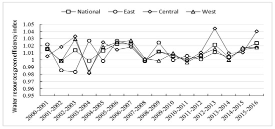
Figure 1.
National and regional changes in water resources green efficiency during the study period 2000–2016.
2. Time-varying characteristics at the regional level
Due to the large expanse of China’s land area, and the great difference of social economic development and climate environment, this paper will divide China into three regional groups: The eastern grouping included 11 provinces (Beijing, Tianjin, Hebei, Liaoning, Shanghai, Jiangsu, Zhejiang, Shandong, Fujian, Guangdong, and Hainan). The central grouping included eight provinces (Shanxi, Jilin, Heilongjiang, Henan, Anhui, Hubei, Hunan, and Jiangxi). The western grouping included 11 provinces (Inner Mongolia, Chongqing, Sichuan, Guizhou, Yunnan, Guangxi, Shaanxi, Gansu, Qinghai, Ningxia and Xinjiang) (the full text of the eastern and western provinces are all the same); according to the level of economic development. As can be seen from Table 2, the water resources green efficiency in the eastern, central and western regions improved during the study period, which is consistent with the conclusion on a national basis. The comparative analysis shows that the greatest efficiency improvement was achieved in the central region, with the efficiency value increasing by 1.4%, followed by that in the western region (1%) and the eastern region (0.9%). However, these results indicate that the difference in the water resources green efficiency among regions was narrow.
In addition, as shown in Figure 1, the trend of water resources green efficiency in the eastern region was negatively correlated with that in the central and western regions before 2007. After 2008, the change trends of water resource green efficiency in the three regions were consistent. The reason is that there is a notable lag in technology transfer. Prior to 2008, as the eastern part of the country was a technology exporter to other areas of the country, thus, while the eastern region improved the water resources green efficiency due to the development and implementation of new technologies, the central and western regions were still applying somewhat outdated production technology. As a result, the water resources green efficiency in these two regions was negatively affected by out-of-date technology compared to technology used in the eastern region. However, after improved technology was transferred from the east to the central and western regions, the trend in efficiency deterioration was curbed. While the eastern region entered the next round of technology research and development, the central and western regions also entered a new round of technical adjustment. During this adjustment, some industries that were harmful to the environment were transferred to the central and western regions. Nevertheless, after 2008, the development and application of clean technologies occurred more widely in the central and western regions, such that the trends in water resources green efficiency in the eastern, central and western regions were similar.
3. Time-varying characteristics at the provincial level
The results presented in Table 2 also show that, except for the efficiencies achieved in Guangxi and Yunnan, the water resources green efficiency of all other provinces improved during the period 2000–2016. (Note: rounding of data resulted in the water resources green efficiency in Liaoning, Fujian, Hainan and Qinghai being interpreted as equal to 1, whereas the original values determined using the HDDF-GML models for these four provinces were actually slightly different, i.e., 1.000008625, 1.0000105, 1.0001125 and 1.002027063, respectively). As can be seen from Table 3, water resources green efficiency in 17 of the 30 provinces improved from 2001 to 2002, deteriorated in 9 of the 30 provinces, and remained unchanged in the other provinces.
Table 3.
Variations in water resources green efficiency index values in provinces during selected years of the study period 2000–2016.
During the period 2005–2006, only the Guangdong, Guangxi, and Qinghai provinces exhibited deteriorating water resources green efficiency. The number of provinces with improved water resources green efficiency increased by five, and the number of provinces with unchanged efficiency values increased by two. However, in 2010–2011, the number of provinces with improved water resources green efficiency decreased to 14, the number of provinces with deteriorating efficiencies increased to 12, and the number of provinces with unchanged water resources green efficiency decreased to four. During 2015–2016, the number of provinces with improved water resources green efficiency increased to 17, whereas the number of provinces with unchanged efficiency reached 10 as in previous years, and the number of provinces with deteriorating efficiency decreased to three.
These results show that, on the one hand, the relationship between water resources green efficiency and economic development was small, and the improvement of water resources green efficiency was also affected by factors in addition to those considered in this study. Thus, it is necessary to further identify all factors affecting the water resources green efficiency. On the other hand, the improvement of water resources green efficiency was variable and prone to relapse, implying that the government must continually formulate and implement effective policies that stimulate and sustain the efficiency improvements. Under the influence of high-quality economic development and ecological civilization construction, achieving the harmonious goals of “economy-society-ecological environment” improvement will be the main challenge in the future development process.
4.1.2. Spatial Differentiation Characteristics of Water Resources Green Efficiency Improvement
(1) Results presented in Table 2 and Figure 2 show that water resources green efficiency improvement was achieved in 14 provinces (Beijing, Shanxi, Inner Mongolia, Jilin, Heilongjiang, Jiangsu, Zhejiang, Anhui, Hubei, Chongqing, Sichuan, Guizhou, Gansu and Ningxia) and nationwide. The degree of efficiency improvement in these 14 provinces exceeded 1.1% and was higher than that at the national level. In contrast, the improvement in water resources green efficiency in 16 other provinces (Tianjin, Hebei, Liaoning, Shanghai, Fujian, Jiangxi, Shandong, Henan, Hunan, Guangdong, Guangxi, Hainan, Yunnan, Shaanxi, Qinghai and Xinjiang) was slower than that at the national level. This difference shows that the water resources green efficiency in most provinces still needs to be improved, and it is necessary to adjust the input–output ratio based on high-quality economic development to improve the green efficiency of water resources.
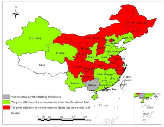
Figure 2.
Average water resource green efficiency improvement (for the 2000–2016 study period) at the provincial level compared to that at the national level.
(2) The top ten provinces in terms of water resources green efficiency improvement during 2000–2016 were Shanxi, Beijing, Inner Mongolia, Jiangsu, Ningxia, Anhui, Heilongjiang, Gansu, Chongqing and Zhejiang. The green efficiency of water resources in these provinces improved faster than the national average. Figure 2 shows that the areas with the fastest improvements in water resources green efficiency were mainly distributed in the western region. This phenomenon may have been due to the absence of water quality issues and serious water pollution in some provinces in the eastern and central regions, while water pollution in the western regions was relatively light and the ecological environment was better than in the east [58]. Moreover, the late-developing advantage of economic development in the western region has made it pay more attention to ecological environment protection, so that the water resources green efficiency improvement in the western region was higher than that in the eastern and central regions. These results also indicate there was no significant positive correlation between the improvement of water resources green efficiency and economic development.
(3) Table 2 and Figure 2 show that the water resources green efficiency in Guangxi has mostly deteriorated over the past 17 years, and improvement in water resources green efficiency in Yunnan, Tianjin and Liaoning was stagnant in most years. In particular, the water resources green efficiency in Yunnan did not change throughout the study period. This stagnation occurred mainly because Guangxi, as one of the 10 non-ferrous metal producing areas in China, pursued economic benefits through extensive mining, resulting in water pollution and ecological environment destruction, and deterioration of water resources green efficiency. As the pillar industries of Yunnan, the tobacco industry, sugar industry and tea industry also cause large environmental problems. However, the importance of water resources to agriculture has enabled the government to strengthen the protection of water resources, effectively stabilizing Yunnan’s water resources green efficiency [59]. Tianjin and Liaoning have well-developed economies. However, due to the inefficient industrial structure and serious population loss, the allocation of resources was unbalanced, resulting in the stagnation of water resources green efficiency in most years.
(4) The improvement of water resources in Hebei, Shandong, Henan, Hunan and Hainan provinces was lower than the national average. However, the improvements were achieved mostly at the expense of the ecological environment. As a result, the social development index of individual regions decreased instead of increasing, resulting in a lower degree of improvement in the water resources green efficiency. These results also emphasize that blindly pursuing economic development while ignoring the development of ecological environment and social benefits may lead to a “bubble” in the form of water utilization efficiency. Therefore, true improvements in water resources green efficiency can be achieved only through high-quality economic development, in which there are rational allocations of resources, efforts to optimize and upgrade the industrial structure, reductions in pollution output and reductions in ecological environment damage.
4.2. Decomposition of Driving Factors for Water Resources Green Efficiency
Based on the mixed directional distance function model, the HDDF-GML index decomposition model was used to explore the driving factors for water resources green efficiency. According to the method of Zofío [46], water resources green efficiency is divided into pure technical efficiency change (PEC) index, scale efficiency change (SEC) index, pure technology change (PTC) index and scale technology change (STC) index. The decomposition results of water resources green efficiency for the period 2000–2016 are shown in Table 4.
Table 4.
Decomposition of the HDDF-GML Index of water resources green efficiency in China for selected years during the study period 2000–2016.
4.2.1. Time-Varying Characteristics of Water Resources Green Efficiency Decomposition
(1) Time-varying characteristics of efficiency decomposition at the national level
As can be seen from Table 4 and Figure 3, firstly, from the perspective of PEC, the national average for the period 2000–2016 was 1.001, an increase of only 0.1%, indicating a slow rising trend in the PEC. Secondly, from the perspective of SEC, the 2000–2016 national average for the period 2000–2016 was 0.9994, which indicated a decrease of 0.06% compared to the value in 2000. An improvement trend in this index was exhibited only in years 2000–2001, 2001–2002, 2003–2004, 2004–2005, 2007–2008, 2010–2011 and 2015–2016. Moreover, in terms of PTC, the national average for the period 2000–2016 was 1.0122, which indicated an increase of 1.22% compared to the value in 2000, and was higher than the increase in the total factor productivity index (1.07%). It shows that PTC has been improving continuously through the 21st century. Finally, in terms of STC, the national average for the period 2000–2016 was 1.0007, indicating an increase of 0.7% in this component since 2000. It showed that water resources scale technology has shown a slow upward trend since 2000.
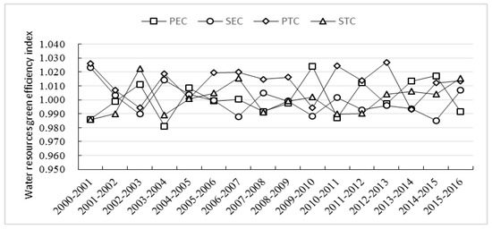
Figure 3.
Changes in components of water resources green efficiency in China during the study period 2000–2016 (PEC = pure technical efficiency change, SEC = scale efficiency change, PTC = pure technology change and STC = scale technology change).
From the perspective of national water resources green efficiency decomposition, the increase in PEC indicates that China can effectively use technological innovation to improve the water resources green efficiency, which means that the current technology application has a positive externality. The largest increase in PTC shows that the improvement of China’s water resources efficiency mainly depends on technological innovation, which may be due to China’s substantial increase in technology research and development expenses in recent years. STC also helps to improve the water resources green efficiency, indicating that technology accumulation in the process of research and development can form a positive scale effect, thereby improving the water resources green efficiency. Where we need to be vigilant is the inhibitory effect of SEC on the water resources green efficiency. The reason for this is that water-saving awareness in water-rich areas is poor, which makes them prone to waste. Generally speaking, while strengthening technology research and development in the future, the country should continue to attach importance to the application of new technologies and tap the potential of existing technologies. This will not only significantly improve the water resources green efficiency, but also help save research and development cost. At the same time, the country urgently needs to strengthen water-saving publicity and policy implementation in areas with abundant water resources to reverse the negative external effects of water resources scale efficiency.
(2) Time-varying characteristics of efficiency decomposition at the regional level
Figure 4 shows that in the eastern region, the PEC of water resources green efficiency greatly improved in 2000–2001 and 2009–2010. SEC decreased much faster in 2006–2007 and 2009–2010 than in other years. PTC showed an upward trend in 2004–2005, but exhibited an abrupt and severe decrease during 2009–2010 that was followed by continuous improvement. STC deteriorated significantly in 2007–2008 and 2010–2011.
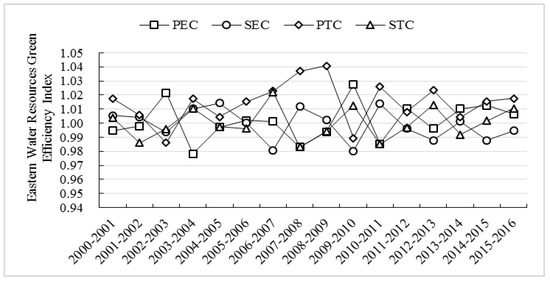
Figure 4.
Changes in components of water resources green efficiency in the eastern region of China during the study period 2000–2016 (PEC = pure technical efficiency change, SEC = scale efficiency change, PTC = pure technology change and STC = scale technology change).
The temporal trend of the decomposition of the water resources green efficiency in central China (Figure 5) showed that PEC significantly increased in 2000–2003 and significantly decreased in 2011–2012. SEC significantly deteriorated in 2000––2003 but markedly improved during 2011–2013. PTC deteriorated significantly in both 2000–2004 and 2012–2014. STC showed significant improvement in 2000–2003, but significant deterioration during the period 2013–2015.
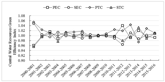
Figure 5.
Changes in components of water resources green efficiency in the central region of China during the study period 2000–2016 (PEC = pure technical efficiency change, SEC = scale efficiency change, PTC = pure technology change and STC = scale technology change).
Variations in components of water resources green energy in the western region are shown in Figure 6. PEC greatly improved during the periods 2003–2005 and 2010–2015. SEC seriously deteriorated in 2000–2003 and 2013–2015. PTC declined in 2003–2005 and 2005–2010. STC reached its highest value in 2002–2003 and the lowest value in 2003–2004.
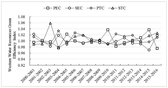
Figure 6.
Changes in the components of water resources green efficiency in the western region of China during the study period 2000–2016 (PEC = pure technical efficiency change, SEC = scale efficiency change, PTC = pure technology change and STC = scale technology change).
Based on the above analysis, it is found that in the process of increasing research and development (R & D) Investment, China should pay more attention to improving the utilization ratio of resources utilization under the existing technological conditions, so as to realize the construction of an innovative country and an environment-friendly society. At the regional level, technological progress in the central and western regions often benefits from technology transfer from the eastern region, making PTC in the central and western regions lag behind that in the eastern region. However, after obtaining advanced technology from the east, the central and western regions have also neglected the role of PEC, SEC and STC. Therefore, in the process of improving water resources green efficiency, all areas of China should increase the funding of R & D and improve the innovation ability of science and technology. More importance should be attached to the application of advanced technologies so as to realize the science-based allocation of human, material and financial resources, and quickly improve the water resources green efficiency level.
4.2.2. Spatial Differentiation Characteristics of Water Resources Green Efficiency Decomposition
(1) Spatial difference analysis of efficiency decomposition at national level
The standard deviation and coefficient of variation of the efficiency decomposition index were calculated for each province from 2000 to 2016, as shown from Figure 7, Figure 8, Figure 9 and Figure 10. The mean variance indicates the absolute difference between provinces, and the coefficient of variation reflects the relative difference between provinces.
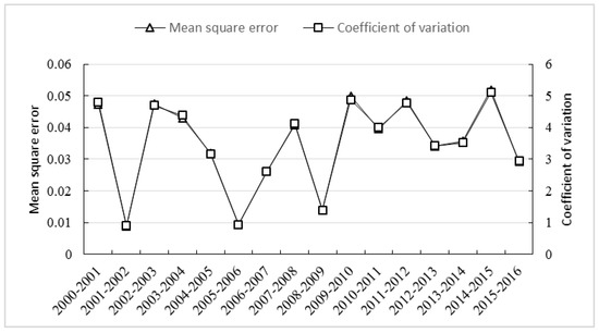
Figure 7.
Changes in average variance and coefficient of variation of PEC.
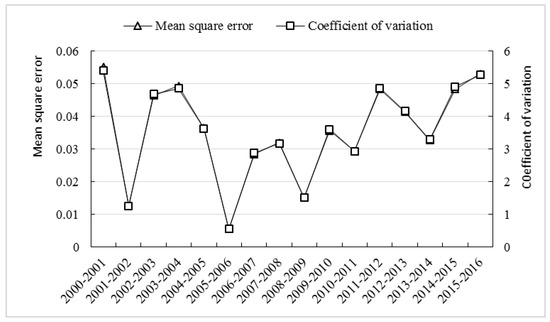
Figure 8.
Changes in average variance and coefficient of variation of SEC.
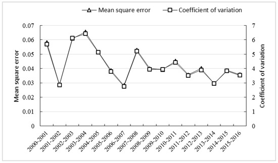
Figure 9.
Changes in average variance and the coefficient of variation of PTC.
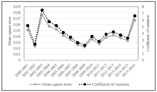
Figure 10.
Changes in average variance and the coefficient of variation of STC.
It can be seen from the figures that the trends of absolute and relative differences in the water resources green efficiency between provinces since 2000 were the same or similar. From the trend of the difference curve between provinces, the trend line of the difference in PEC between provinces fluctuated first before increasing and then decreasing (Figure 7). The difference in SEC between provinces was small (Figure 8), and the difference in STC was increasing (Figure 10). The difference in PTC fluctuated first and then decreasing steadily (Figure 9). All four indicators showed that the ability of Chinese provinces to master frontier technology gradually decreased, and the scale effect in different provinces was quite different. Therefore, at the national level, it is necessary to further improve the efficiency and scale effect of technological change to realize coordinated development among provinces and the spatial balance of water requirements.
(2) Spatial difference analysis of efficiency decomposition at provincial level
As can be seen from Table 5, only Tianjin, Qinghai, Gansu and Guizhou among the 30 provinces in the country have not improved in PTC. The proportions of provinces in which PEC, SEC, and STC indices improved were 40%, 46.67%, and 60%, respectively. This conclusion is consistent with the characteristics of the time change of each index.
Table 5.
GML index decomposition interval division by province during the study period 2000–2016.
By further analysis of Figure 11, it is found that the five provinces with the largest increase and decrease in PEC in the study period were mainly located in central and western provinces, while the central and eastern coastal provinces where PEC remained unchanged account for 57.14%. The five provinces with the largest increase and decrease in SEC were also mainly located in the central and western provinces. Specifically, it mainly includes Sichuan and Yunnan in the west, Hubei, Anhui, and Jilin in the central, and Jiangsu in the east. While the scale effect of technological changes improved in most of China.
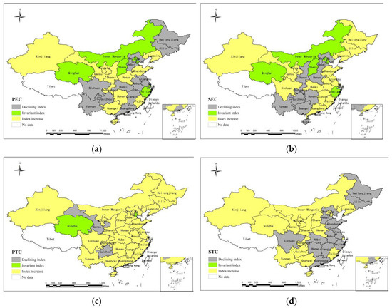
Figure 11.
Spatial differentiation characteristics of water resource green efficiency index: (a) Spatial differentiation of pure technology efficiency change (PEC), (b) Spatial differentiation of scale efficiency change (SEC), (c) Spatial differentiation of pure technology change (PTC) and (d) Spatial differentiation of scale technology change (STC).
These results may be due to the fact that the eastern coastal provinces early paid attention to the innovation of environmental protection technologies and equipment. However, there is still a certain gap between the technical efficiency of the developed eastern provinces and that of the western developed countries, leading to low-level repetitive investment and a decline in the scale effect of technological efficiency, which leads to low-level repeated investment. This is also an urgent problem to be solved in the process of realizing the green development of social economy in the future.
Most of the central provinces are home to (mainly) heavy industries, which are slow to respond to the innovation of pure technical efficiency, which has led to a decline in the PEC. However, some central provinces have seized the policy dividend of “the rise of central China” to optimize and upgrade their industrial structure and improve pure technical efficiency. Most western provinces can avail of the “late-development advantage” to avoid low level investment and construction, and improve the PEC of production. However, a few western provinces are temporarily unable to quickly improve PEC due to the inertia of economic development and poor natural conditions.
It can be seen from the analysis of spatial differentiation characteristics that the improvement of water resources green efficiency in China has been mainly due to the improvement of pure technology, such that PEC and STC have relatively less impetus. SEC appears to hinder the effect. Technological progress has promoted the improvement of water resources green efficiency in China, which is in line with the theoretical hypothesis that “technology will not be forgotten” with regard to frontier technologies, as espoused by Henderson [60]. The results from this study also are consistent with the empirical results in most of the relevant literature [61].
5. Conclusions and Recommendations
5.1. Conclusions
This study utilized the HDDF-GML index model under from the perspective of mixed disposability to evaluate the dynamic changes of water resources green efficiency in China from 2000 to 2016. Furthermore, Zofío’s [46] decomposition method was used to study the inherent driving factors of water resources green efficiency. The main conclusions are as follows:
Firstly, in terms of the time-varying characteristics of water resources green efficiency improvement, water resources green efficiency has improved overall (by 1.1%) between 2000 and 2016. The efficiency has improved the most in China’s central region, with an increase of 1.4%, followed by that in the western region (1%), and the eastern region (0.9%). On a provincial level, the water resources green efficiency has improved in all provinces except Guangxi and Yunnan. In different time periods, the number of provinces in which the water resources green efficiency has improved, deteriorated and unchanged has increased.
Secondly, in terms of the spatial differentiation of water resources green efficiency improvement, the efficiencies in 14 provinces (Beijing, Shanxi, Inner Mongolia, Jilin, Heilongjiang, Jiangsu, Zhejiang, Anhui, Hubei, Chongqing, Sichuan, Guizhou, Gansu and Ningxia) are higher than the national level. In contrast, the rate of water resources green efficiency improvement in Tianjin, Hebei, Liaoning, Shanghai, Fujian, Jiangxi, Shandong, Henan, Hunan, Guangdong, Guangxi, Hainan, Yunnan, Shaanxi, Qinghai and Xinjiang is lower than the national level. The top ten provinces for improvement are Shanxi, Beijing, Inner Mongolia, Jiangsu, Ningxia, Anhui, Heilongjiang, Gansu, Chongqing and Zhejiang. From spatio-temporal analysis of green efficiency of water resources, it can be found that water resources green efficiency is significantly affected by national policies, but there may not be a significant positive correlation with economic development. At present, the water resources green efficiency in most provinces still needs to be improved.
Thirdly, in terms of time-varying characteristics of water resources green efficiency decomposition, SEC has declined during 2000–2016 but the other three indices have increased. PTC is increasing faster than PEC and STC. Provinces in the eastern, central and western regions, as well as China nationally, should pay more attention to improving resource utilization under existing technical conditions in the process of increasing R & D investment.
Finally, in terms of spatial differentiation characteristics of water resources green efficiency decomposition, the absolute and relative differences in water resources green efficiency among provinces since 2000 have been the same or similar. The inter-provincial differences of PEC are variable, and have decreased before increasing and then decreasing again. In contrast, the differences of SEC and STC have shown overall upward trends, and the difference of the PTC have decreased steadily after an initial increase. Except for Tianjin City and Qinghai, Gansu and Guizhou provinces, where the PTC is unchanged or decreasing, all other provinces are in a state of improvement. The proportions of provinces that exhibit improved PEC, SEC, and STC are 40%, 46.67%, and 60%, respectively.
5.2. Recommendations
Based on the above conclusions, the following recommendations are made.
(1) Establish a circular economy development model to achieve simultaneous economic-social-ecological goals. First, in the process of economic development, the ecological economic development model of “resource source control, supplemented by pollution end management” should be implemented. The scope of clean energy should be expanded and the “pollution first and treatment later” model should be abandoned. Second, strengthen the process control of social and economic development, improve the degree of resource recycling, and use resources to make “reduce, reuse, recycle” the production code of conduct, so that the economic system and the material cycle of the ecosystem are coordinated. Finally, strengthen results control, encourage residents to consume green products, improve social recognition of green products, and develop a functional and sharing economy so as to make full use of excess capacity, promote supply-side structural reform, achieve economic “connotative” development, and thereby improve the water resources green efficiency.
(2) Increase investment in R & D and enhance independent innovation capabilities. At the national level, the government should improve the environment for scientific and technological innovation through the combination of market mechanisms and administrative management, strengthen intellectual property protection, and increase the enthusiasm of independent research and development. Financial instruments should be used to increase financial support for independent innovation, and especially to strengthen financial support for high-technology and environmentally friendly industries. The government should introduce social forces, strengthen its supervision of R & D investment costs, ensure earmarking, and help increase R & D output rate. Domestic scientific and technological talents should be cultivated, and leading international talents should be introduced in science and technology, while improving the initiative of R & D talents and promoting green technology. Thus establish and promote a sound scientific and technological innovation system for building an innovative country. At the provincial level, less-developed provinces should quickly encourage enterprises to increase the investment of R & D funds according to their own economic foundation and industrial structure. Furthermore, central transfer payments should be used to increase financial support for independent innovation and increase corporate enthusiasm for R & D investment. The situation should be avoided that the development of enterprises is hindered by excessive R & D investment, so as to realize the effect of increasing R & D investment in water resources green efficiency.
(3) Introduce technology in an orderly manner and increase the rate of technology introduction and conversion. The process of independent innovation includes not only original technological innovation, but also the transformation of foreign advanced technologies. Through learning and absorbing foreign advanced technologies, new technologies that meet the needs of China’s social and economic development can be formed. Therefore, in the process of technology introduction, it is necessary to not only ensure that the advanced technology is appropriate, but also that it is adaptable. In addition, the local conversion rate of foreign advanced technology must improve, thereby achieving the purpose of promoting domestic technological progress, and ultimately improving water resources green efficiency.
(4) Balance technical efficiency and scale efficiency. In the process of strengthening independent innovation and technology introduction, more attention should be paid to improving technology efficiency and scale efficiency, thereby improving resource utilization efficiency and scale efficiency of resource input through existing technical conditions. In addition, in the process of promoting technological progress, attention should also be paid to increases in the scale of technology and understanding that technological progress has a scale effect, so that scientific and technological innovation can better promote water resources green efficiency.
Author Contributions
Conceptualization, H.Z. and H.C.; Methodology, H.Z. and H.C.; Software, G.M.; Validation, H.Z., H.C. and M.W.; Formal Analysis, H.Z.; Investigation, H.Z.; Data Curation, H.Z. and W.J.; Writing—Original Draft Preparation, H.Z.; Writing—Review and Editing, M.W. and W.J.; Resources: R.L.; Visualization, G.M.; Supervision, H.C.; Project Administration, R.L.; Funding Acquisition, R.L. and W.J. All authors have read and agreed to the published version of the manuscript.
Funding
This study was funded by the Major Project of National Social Science Foundation of China (No.19ZDA107), the Key Project of National Social Science Foundation of China (No.18AZD014) and the Youth Fund Project of Humanities and Social Sciences Research of Education Ministry (No.18YJC790065).
Acknowledgments
This study was financially supported by the Youth Fund Project of Humanities and Social Sciences Research of Education Ministry (No.18YJC790065) and the Key Project of National Social Science Foundation of China (No.18AZD014).
Conflicts of Interest
The authors declare no conflict of interest.
References
- Wada, Y.; De Graaf, I.E.M.; Van Beek, L.P.H. High-resolution modeling of human and climate impacts on global water resources. J. Adv. Model. Earth Syst. 2016, 8, 735–763. [Google Scholar] [CrossRef]
- The United Nations World Water Assessment Programme. The United Nations World Water Development Report 2014: Water and Energy; UNESCO: Paris, France, 2014. [Google Scholar]
- Jia, S.F.; Zhang, J. Institutional reform of water resources management in China. China Popul. Res. Environ. 2011, 21, 102–106. (In Chinese) [Google Scholar] [CrossRef]
- Nabi, G.; Ali, M.; Khan, S.; Kumar, S. The crisis of water shortage and pollution in Pakistan: Risk to public health, biodiversity, and ecosystem. Environ. Sci. Pollut. Res. 2019, 26, 10443–10445. [Google Scholar] [CrossRef] [PubMed]
- Thoradeniya, B.; Pinto, U.; Maheshwari, B. Perspectives on impacts of water quality on agriculture and community well-being—A key informant study from Sri Lanka. Environ. Sci. Pollut. Res. 2017, 26, 2047–2061. [Google Scholar] [CrossRef]
- Wenter, A.; Zanotelli, D.; Montagnani, L.; Tagliavini, M.; Andreotti, C. Effect of different timings and intensities of water stress on yield and berry composition of grapevine (cv. Sauvignon blanc) in a mountain environment. Sci. Hortic. 2018, 236, 137–145. [Google Scholar] [CrossRef]
- Legesse, G.; Cordeiro, M.R.C.; Ominski, K.H.; Beauchemin, K.A.; Kröbel, R.; McGeough, E.; Pogue, S.; McAllister, T.A. Water use intensity of Canadian beef production in 1981 as compared to 2011. Sci. Total. Environ. 2018, 619, 1030–1039. [Google Scholar] [CrossRef]
- Yawen, Z.X.L. Changes and mechanism of internal water use of products in Tianjin. Res. Sci. 2016, 38, 52–63. [Google Scholar] [CrossRef]
- Kopp, R.J. The Measurement of Productive Efficiency: A Reconsideration. Q. J. Econ. 1981, 96, 477. [Google Scholar] [CrossRef]
- Lei, Y.T.; Huang, L.P.; Zhang, H. Research on the dynamic evolution and the driving factors of industrial water consumption efficiency in China. Res. Environ. Yangtze Basin. 2017, 26, 159–170. (In Chinese) [Google Scholar] [CrossRef]
- Mellah, T.; Ben Amor, T. Performance of the Tunisian Water Utility: An input-distance function approach. Util. Policy 2016, 38, 18–32. [Google Scholar] [CrossRef]
- Guerrini, A.; Romano, G.; Leardini, C. Economies of scale and density in the Italian water industry: A stochastic frontier approach. Util. Policy 2018, 52, 103–111. [Google Scholar] [CrossRef]
- Gadanakis, Y.; Bennett, R.; Park, J.; Areal, F.J. Improving productivity and water use efficiency: A case study of farms in England. Agric. Water Manag. 2015, 160, 22–32. [Google Scholar] [CrossRef]
- Morales, M.; Heaney, J. Benchmarking Nonresidential Water Use Efficiency Using Parcel-Level Data. J. Water Resour. Plan. Manag. 2016, 142, 04015064. [Google Scholar] [CrossRef]
- Tone, K. A slacks-based measure of efficiency in data envelopment analysis. Eur. J. Oper. Res. 2001, 130, 498–509. [Google Scholar] [CrossRef]
- Jin, W.; Liu, S.S.; Zhang, K.; Kong, W. Influence of agricultural production efficiency on agricultural water consumption. J. Nat. Res. 2018, 33, 1326–1339. (In Chinese) [Google Scholar] [CrossRef]
- Färe, R.; Njinkeu, D. Computing returns to scale under alternative models. Econ. Lett. 1989, 30, 55–59. [Google Scholar] [CrossRef]
- Yang, W.; Li, L. Analysis of Total Factor Efficiency of Water Resource and Energy in China: A Study Based on DEA-SBM Model. Sustainability 2017, 9, 1316. [Google Scholar] [CrossRef]
- Rolfe, J.; Windle, J.; McCosker, K.; Northey, A. Assessing cost-effectiveness when environmental benefits are bundled: Agricultural water management in Great Barrier Reef catchments. Aust. J. Agric. Resour. Econ. 2018, 62, 373–393. [Google Scholar] [CrossRef]
- Lorenzo-Toja, Y.; Vázquez-Rowe, I.; Marín-Navarro, D.; Crujeiras, R.M.; Moreira, M.T.; Feijoo, G. Dynamic environmental efficiency assessment for wastewater treatment plants. Int. J. Life Cycle Assess. 2017, 23, 357–367. [Google Scholar] [CrossRef]
- Shi, T.; Zhang, X.; Du, H.; Shi, H. Urban water resource utilization efficiency in China. Chin. Geogr. Sci. 2015, 25, 684–697. [Google Scholar] [CrossRef]
- Maziotis, A.; Molinos-Senante, M.; Sala-Garrido, R. Assesing the Impact of Quality of Service on the Productivity of Water Industry: A Malmquist-Luenberger Approach for England and Wales. Water Resour. Manag. 2016, 31, 2407–2427. [Google Scholar] [CrossRef]
- Song, M.; Wang, R.; Zeng, X. Water resources utilization efficiency and influence factors under environmental restrictions. J. Clean. Prod. 2018, 184, 611–621. [Google Scholar] [CrossRef]
- Huang, R.; Li, Y. Undesirable input–output two-phase DEA model in an environmental performance audit. Math. Comput. Model. 2013, 58, 971–979. [Google Scholar] [CrossRef]
- Worthington, A.C. A review of frontier approaches to efficiency and productivity measurement in urban water utilities. Urban Water J. 2013, 11, 55–73. [Google Scholar] [CrossRef]
- Wang, S.; Zhou, L.; Wang, H.; Li, X. Water Use Efficiency and Its Influencing Factors in China: Based on the Data Envelopment Analysis (DEA)—Tobit Model. Water 2018, 10, 832. [Google Scholar] [CrossRef]
- Zhao, L.; Sun, C.; Liu, F. Interprovincial two-stage water resource utilization efficiency under environmental constraint and spatial spillover effects in China. J. Clean. Prod. 2017, 164, 715–725. [Google Scholar] [CrossRef]
- Li, J.; Ma, X.-C. Econometric analysis of industrial water use efficiency in China. Environ. Dev. Sustain. 2014, 17, 1209–1226. [Google Scholar] [CrossRef]
- Wang, Y.; Bian, Y.; Xu, H. Water use efficiency and related pollutants’ abatement costs of regional industrial systems in China: A slacks-based measure approach. J. Clean. Prod. 2015, 101, 301–310. [Google Scholar] [CrossRef]
- Che, L.; Bai, Y.P.; Zhou, L.; Wang, F.; Ji, X.M.; Qiao, F.W. Spatial pattern and spillover effects of green development efficiency in China. Sci. Geogr. Sin. 2018, 38, 1788–1798. (In Chinese) [Google Scholar] [CrossRef]
- Jin, W.; Zhang, H.-Q.; Liu, S.-S.; Zhang, H.-B. Technological innovation, environmental regulation, and green total factor efficiency of industrial water resources. J. Clean. Prod. 2019, 211, 61–69. [Google Scholar] [CrossRef]
- Fu, J.; Xiao, G.; Guo, L.; Wu, C. Measuring the Dynamic Efficiency of Regional Industrial Green Transformation in China. Sustainability 2018, 10, 628. [Google Scholar] [CrossRef]
- Geng, Y.; Wang, M.; Sarkis, J.; Xue, B.; Zhang, L.; Fujita, T.; Yu, X.; Ren, W.; Zhang, L.; Dong, H. Spatial-temporal patterns and driving factors for industrial wastewater emission in China. J. Clean. Prod. 2014, 76, 116–124. [Google Scholar] [CrossRef]
- Shang, Y.; Lu, S.; Li, X.; Sun, G.; Shang, L.; Shi, H.; Lei, X.; Ye, Y.; Sang, X.; Wang, H. Drivers of industrial water use during 2003–2012 in Tianjin, China: A structural decomposition analysis. J. Clean. Prod. 2017, 140, 1136–1147. [Google Scholar] [CrossRef]
- Sun, C.; Zhao, L.; Zou, W.; Zheng, D.-F. Water resource utilization efficiency and spatial spillover effects in China. J. Geogr. Sci. 2014, 24, 771–788. [Google Scholar] [CrossRef]
- Ma, H.; Shi, C.; Chou, N.-T. China’s Water Utilization Efficiency: An Analysis with Environmental Considerations. Sustainablity 2016, 8, 516. [Google Scholar] [CrossRef]
- Li, Y.L.; Wu, C. Random DEA model considering the weak disposability of undesirable outputs. J. Manag. Sci. China 2014, 17, 17–28. (In Chinese) [Google Scholar] [CrossRef]
- Xue, S.; Yang, T.; Zhang, K.; Feng, J. Spatial effect and influencing factors of agricultural water enivronmental efficiency in China. Appl. Ecol. Environ. Res. 2018, 16, 4491–4504. [Google Scholar] [CrossRef]
- Charnes, A.; Cooper, W.; Rhodes, E. Measuring the efficiency of decision making units. Eur. J. Oper. Res. 1978, 2, 429–444. [Google Scholar] [CrossRef]
- Zhou, X.; Luo, R.; Yao, L.; Cao, S.; Wang, S.; Lev, B. Assessing integrated water use and wastewater treatment systems in China: A mixed network structure two-stage SBM DEA model. J. Clean. Prod. 2018, 185, 533–546. [Google Scholar] [CrossRef]
- Färe, R.; Grosskopf, S. Directional distance functions and slacks-based measures of efficiency: Some clarifications. Eur. J. Oper. Res. 2010, 206, 702. [Google Scholar] [CrossRef]
- Tone, K. A Hybrid Measure of Efficiency in DEA; GRIPS Policy Information Center Research Report; National Graduate Institute for Policy Studies: Tokyo, Japan, 2004. [Google Scholar]
- Cheng, G. Data Development Analysis: Methods and MaxDEA Software; Intellectual Property Publishing House: Beijing, China, 2017. [Google Scholar]
- Chung, Y.; Färe, R.; Grosskopf, S. Productivity and Undesirable Outputs: A Directional Distance Function Approach. J. Environ. Manag. 1997, 51, 229–240. [Google Scholar] [CrossRef]
- Oh, D.-H. A global Malmquist-Luenberger productivity index. J. Prod. Anal. 2010, 34, 183–197. [Google Scholar] [CrossRef]
- Zofío, J.L. Malmquist productivity index decompositions: A unifying framework. Appl. Econ. 2007, 39, 2371–2387. [Google Scholar] [CrossRef]
- Shan, H.J. Reestimating the capital stock of China: 1952–2006. J. Quant. Tech. Econ. 2008, 10, 17–31. (In Chinese) [Google Scholar] [CrossRef]
- Medrano, H.; Tomás, M.; Martorell, S.; Escalona, J.-M.; Pou, A.; Fuentes, S.; Flexas, J.; Bota, J. Improving water use efficiency of vineyards in semi-arid regions. A review. Agron. Sustain. Dev. 2014, 35, 499–517. [Google Scholar] [CrossRef]
- Urpelainen, J. Export orientation and domestic electricity generation: Effects on energy efficiency innovation in select sectors. Energy Policy 2011, 39, 5638–5646. [Google Scholar] [CrossRef]
- Stern, D.I. Modeling international trends in energy efficiency. Energy Econ. 2012, 34, 2200–2208. [Google Scholar] [CrossRef]
- Chhipi-Shrestha, G.; Hewage, K.; Sadiq, R. Water–Energy–Carbon Nexus Modeling for Urban Water Systems: System Dynamics Approach. J. Water Resour. Plan. Manag. 2017, 143, 04017016. [Google Scholar] [CrossRef]
- Yousefi, M.; Khoramivafa, M.; Damghani, A.M. Water footprint and carbon footprint of the energy consumption in sunflower agroecosystems. Environ. Sci. Pollut. Res. 2017, 24, 19827–19834. [Google Scholar] [CrossRef]
- Xu, J. Coupling mechanism of regional carbon-water symbiosis system and water resources regulation and control under low carbon perspective. Appl. Ecol. Environ. Res. 2017, 15, 457–465. [Google Scholar] [CrossRef]
- Sun, C.Z.; Jiang, K.; Zhao, L.S. Measurement of green efficiency of water utilization and its spatial pattern in China. J. Nat. Res. 2017, 32, 1999–2011. (In Chinese) [Google Scholar] [CrossRef]
- Lai, S.Y.; Du, P.F.; Chen, J.N. Evaluation of non-point source pollution based on unit analysis. J. Tsinghua Univ. 2004, 44, 1184–1187. [Google Scholar] [CrossRef]
- Chen, S.; Shiyi, C. Engine or drag: Can high energy consumption and CO2 emission drive the sustainable development of Chinese industry? Front. Econ. China 2009, 4, 548–571. [Google Scholar] [CrossRef]
- Xiong, Y.; Peng, S.; Luo, Y.; Xu, J.; Yang, S. A paddy eco-ditch and wetland system to reduce non-point source pollution from rice-based production system while maintaining water use efficiency. Environ. Sci. Pollut. Res. 2014, 22, 4406–4417. [Google Scholar] [CrossRef]
- Sun, C.Z.; Ma, Q.F.; Zhao, L.S. Green efficiency changes for water resources in china based on SBM-Malmquist model. Res. Sci. 2018, 40, 993–1005. (In Chinese) [Google Scholar] [CrossRef]
- Liu, S.S.; Han, F.M.; Cai, A.N.; Zhang, K.; Jin, W. Influence of agricultural water use efficiency on agricultural water consumption in consideration of regional differences. Res. Environ. Yangtze Basin 2017, 26, 2099–2110. (In Chinese) [Google Scholar] [CrossRef]
- Henderson, A.R. The bootstrap: A technique for data-driven statistics. Using computer-intensive analyses to explore experimental data. Clin. Chim. Acta 2005, 359, 1–26. [Google Scholar] [CrossRef]
- Hu, B.; Wang, F.; Li, J.Y.; Yu, L.Y.; Zhang, S.H. Efficiency evaluation on urban eco-civilization construction via SBM-Undesirable Model-Taking Tianjin as an example. J. Arid Land Res. Environ. 2015, 29, 13–18. (In Chinese) [Google Scholar] [CrossRef]


© 2020 by the authors. Licensee MDPI, Basel, Switzerland. This article is an open access article distributed under the terms and conditions of the Creative Commons Attribution (CC BY) license (http://creativecommons.org/licenses/by/4.0/).