Abstract
The paper presents a new approach to identify the unknown characteristics (release history and location) of contaminant sources in groundwater, starting from a few concentration observations at monitoring points. An inverse method that combines the forward model and an optimization algorithm is presented. To speed up the computation, the transfer function theory is applied to create a surrogate transport forward model. The performance of the developed approach is evaluated on two case studies (literature and a new one) under different scenarios and measurement error conditions. The literature case study regards a heterogeneous confined aquifer, while the proposed case study was never investigated before, it involves an aquifer-river integrated flow and transport system. In this case, the groundwater contaminant originated from a damaged tank, migrates to a river through the aquifer. The approach, starting from few concentration observations monitored at a downstream river cross-section, accurately estimates the release history at a groundwater contaminant source, even in presence of noise on observations. Moreover, the results show that the methodology is very fast, and can solve the inverse problem in much less computation time in comparison with other existing approaches.
1. Introduction
The problem of the identification of a contaminant source has attracted the attention of many researchers in recent decades. Although many approaches have been developed so far, no definite cure has yet been proposed. This is due to its ill-posed nature together with scarce, frequently also inaccurate data [1]. There are three main approaches to solve numerically the problem of contaminant source identification: mathematical, probabilistic, and simulation—optimization. In the mathematical method, the governing contaminant transport equation is first solved, and then, considering the superposition principle, the final solution, which includes all involved sources, is obtained. Since this approach leads to a linear, ill-posed algebraic system of equations, regularization methods are used for overcoming the ill-posed condition [2]. Skaggs and Kabala [3] were the pioneers in this approach; they recovered the release history of a groundwater contaminant originating from a known, single source and applied Tikhonov regularization (TR) in numerical experiments for improving the ill-posed condition of the system. Skaggs and Kabala [3] showed that the method performance is significantly affected by the measurement errors of the input data. The method of quasi-reversibility (QR) [4] was applied to recover the release history of the groundwater contaminant plume. The results showed that the implementation of the QR method is easier but less accurate than the TR method. Liu and Ball [5] used a least-squares method modified by adding a Tikhonov regularization term to estimate the groundwater contaminant source release history. It is notable that the mathematics formulation takes much less consuming time, but it is more complex than other methods. Moreover, probabilistic and geostatistical methods have attracted researchers’ attention to identifying the characteristics of the contaminant sources. The most important feature of this approach is that including the problem in a stochastic framework, the parameters to estimate become random variables. In this method, unknowns are discovered without the use of iterative methods, or at least with fewer iterations than the optimization method. This approach was developed by Bagtzoglou et al. [6]. They solved the transport equation to estimate the groundwater contaminant source location and release history using the random walk particle method. Liu and Wilson [7] introduced the backward probabilities method to solve the contaminant transport equation in a two-dimensional heterogeneous aquifer. Woodbury and Ulrych [8] used the minimum relative entropy (MRE) approach to recover the release and evolution histories of a plume in a groundwater one-dimensional system with constant known dispersivity and uniform velocity. Cupola et al. [9] extended the MRE approach to 2-D domains. Neupauer and Wilson [10,11] developed a backward probability model based on the adjoint state method (BPM-ASM) to identify the source location of a conservative contaminant release in the one-dimensional domain [10], two- dimensional domain [11] and of a non-conservative pollutant (first-order decay) in the one-dimensional domain [12]. Neupauer et al. [13], compared the results of Tikhonov regularization (TR) to the one of minimum relative entropy (MRE) in the recovery of the release history of a conservative contaminant in a one-dimensional domain. The results showed the MRE method is more robust than TR in error-free data condition, but the TR method is better if there is an error in data. Snodgrass and Kitanidis [14] developed an efficient geostatistical method to estimate the contaminant source release, considering the source location known. Michalak and Kitanidis [15] applied a geostatistical approach combined with the adjoint state method for the recovery of historical groundwater contaminant distribution. By using this approach, the groundwater contaminant release history can be recovered, even in the heterogeneous domain. Boano et al. [16] applied a geostatistical method to identify the release history of contaminant source with a linear decay reaction using a finite number of concentration data located at a known location in a river. Butera et al. [17] employed a simultaneous release history and source location identification methodology (SRSI) to identify the groundwater pollution source location and the release history. Gzyl et al. [18] applied a multi-step approach to identify groundwater contaminant source and release history in a real field case study. Their approach consists of three steps: performing integral pumping tests, identifying sources, and recovering the release history using a geostatistical method. Cupola et al. [19] evaluated the relative effectiveness of two methods: SRSI and BPM-ASM using data collected through sandbox experiments. The results showed the effective performance of both methods. However, the SRSI method requires some weak hypotheses regarding the statistical structure of the unknown release function and a preliminary definition of the probable source location. In addition, BPM-ASM needs to assume some hypotheses about the contaminant release time in the backward probability model. Recently, the group of Gómez-Hernández developed a new approach based on Kalman filter to estimate the source release, its location, and aquifer properties [20,21,22]. The last category of inverse problem solution method is the simulation–optimization approach. The optimization method consists of the integration of both simulation and optimization models. The main purpose of simulation models is to solve the governing flow and transport equations for given initial and boundary conditions. However, these models are not capable of obtaining the inverse solution. In order to identify the input of the forward model that best fits the observed data, these models have to be integrated with optimization procedures. This approach has a simplicity of formulation—it is one of the most widely used by researchers—but the computational cost is relatively high. Certainly, Gorelick [23] was among the first in identifying the characteristic of groundwater contaminant source (locations and intensity of pollutant sources) using linear programming and the least squares regression. Datta et al. [24] developed a new methodology, based on a pattern-recognition algorithm, to identify unknown groundwater pollution source locations and intensities by using Bayes’ optimal decision rule to achieve this purpose. Wagner [25] presented a methodology based on a non-linear maximum likelihood method for simultaneous estimation of aquifer parameters and source characteristics. Mahar and Datta [26,27] used an embedded nonlinear optimization model to identify the characteristics of unknown groundwater pollution sources. Mahar and Datta [26] obtained preliminary identification of source location in the first phase, the duration of the activity and intensity, using an embedded optimization technique. In the second step, an optimal monitoring network design was presented using the preliminary identification results; in the final step, unknown source characteristics were recovered with new data set at the designed monitoring well locations. They also presented the embedded nonlinear optimization model to determine simultaneously unknown groundwater pollution sources and aquifer parameters [27]. Aral et al. [28] formulated a modified version of the genetic algorithm namely, the progressive genetic algorithm to identify unknown contaminant source location and release histories. Sun et al. [29] introduced a new framework (constrained robust least squares, CRLS), which is a new version of RLS, for recovering the release history of contaminant sources. The performance of CRLS model is evaluated through one- and two- dimensional test cases, which showed the model performance is better than RLS, while the system is ill-posed and uncertain. Ayvaz [30] proposed a linked simulation–optimization model to recover the release histories and to determine the locations of the groundwater contaminant sources. He applied the heuristic harmony search algorithm in the optimization model.
The optimization procedure bases on an iterative procedure that requires many forward model runs. Several approaches, such as surrogate modeling, are available to improve the simulation model efficiency by reducing the forward model computation time. The most important surrogate model can be framed in the data-driven model category, see Table 1 for a summary.

Table 1.
Summary of data-driven models and related references.
Groundwater (GW) and surface water (SW) are components of the hydrological cycle that mutually affect each other. So far, various models were created to investigate the hydrological behavior of GW-SW integrated systems [51,52,53]. However, with the progress of computers and the increase of their speed and computational power, models are now capable of coupling surface hydrodynamic systems to groundwater [54,55,56,57,58].
To evaluate the performance of the presented approach, two main case studies with some scenarios are considered. The first one is a literature case study [30,48] that consists of a two-dimensional heterogeneous aquifer with two contaminant sources and seven monitoring wells. The second one is a complex hypothetical case study including an aquifer-river integrated system that presents polluted surface water originated by the groundwater contaminant migration of the leakage from a damaged underground tank. A detailed inspection of the studies conducted in the field of contaminant source identification indicates that all of them are applied only in groundwater or rivers, and no studies have been undertaken to consider, in the inverse modeling procedure, both river, and groundwater domains, with mutual interaction. In other words, in all coupled models of groundwater and surface water, flow and transport equations are solved in a forward way. Therefore, a methodology that can solve inverse problems in the integrated domains of the aquifer and river is of interest. In particular, the inverse problem analyzed in this paper consists of the estimate of the contaminant source location and release history in the groundwater and groundwater-river domains. A simulation–optimization approach based on a surrogate transport model has been applied. The transfer function theory is used to create surrogate transport model. It is convenient, very fast compared to other existing approaches and the output can be easily determined for any given input. Another advantage is that governing complex differential and integral equations are transformed into simple and easy algebraic equations. Therefore, it can be used for real scenarios of pollutant transport problems. The other important issue is that the problem of aquifer-river system is a novel one, and it has been investigated for the first time in this study by the transfer function approach.
For all cases and scenarios, the related statistical parameters are obtained and analyzed in terms of accuracy and effectiveness. The structure of the present paper is as follows: In Section 2, details of the applied methods and performance metrics are given. In Section 3, the test cases and results are shown. Finally, the conclusion is introduced in the fourth section.
2. Mathematical statements
2.1. Flow and Contaminant Transport Equations in Groundwater
For the sake of simplicity, let us consider two-dimensional flow in a confined aquifer with known hydraulic parameters. It has to be noted, that the developments presented hereafter can be generalizable to three-dimensional aquifers, in either confined or unconfined systems. To solve uncoupled contaminant transport problems known velocity field is required. Then, it is necessary to determine the groundwater flow field. Equation (1) shows the two-dimensional water balance, including the Darcy law, in a heterogeneous anisotropic confined aquifer [59].
where and are values of the principal components of the transmissivity tensor in and directions [], respectively; is the piezometric head []; is the volumetric flux per unit area sources or sinks of water []; is the storativity of the porous material [-] and is the time []. The symbols used in this paper are listed in the Supplementary Materials.
Equation (2) describes the transport process in an aquifer with the injection of a non-sorbing, non-reactive solute at a point source [59]:
where is a vector describing the point location in the two-dimensional domain, [-] is the effective porosity, [LT−1] is the effective velocity at location and time [T], [L2T−1] is the dispersion tensor, [ML−3] is the concentration at location and time , is the differential operator Nabla and s(t) [MT−1] is the amount of contaminant per unit time injected into the aquifer through the source located at and δ [L−3] is Dirac delta function.
2.2. Transfer Function Theory in Groundwater
The solution of the linear differential Equation (2) considering the initial and boundary conditions ; , is given by the following convolution integral [60]:
where g(x, t − τ) is the transfer (kernel) function that describes the effects at the location and time by an impulse injection occurring at location and time τ. In complex flow conditions, such as non-uniform flow fields and non-isotropic and heterogeneous aquifers, there is no analytical solution of the transfer function, thus, the use of numerical approaches is unavoidable. The stepwise input function procedure methodology [17,49] is one of the best numerical strategies for the Kernel functions calculation. It is shortly described as follows:
Considering a simple variable transformation τ = t − τ, Equation (3) can be rewritten as:
Assuming a stepwise input function as s(t − τ) = F0· H(t − τ) where H(t − τ) [-] is the Heaviside step function (for t − τ > 0 it is equal to unity) and F0 [] is the amount of pollutant per unit time injected into the aquifer, after taking the time derivative of Equation (4), results in [17]:
The concept of Equation (5) is that the transfer function at a generic point can be calculated from the derivative of the breakthrough curve (concentration history) at the same location , due to a stepwise contaminant injection at the location x0. Under field conditions, it is rarely possible to determine the response of an aquifer due to an indefinite step injection, because it has a very long experimentation time. However, a calibrated numerical flow and transport model are often available, and can easily simulate the effect of a contaminant injection on an aquifer and calculate its response at each monitoring point. Accordingly, the breakthrough curves in different locations and their numerical derivative can be determined to solve the inverse problems. Figure 1 shows the schematic of a dimensionless breakthrough curve and its derivative named transfer function (TF).

Figure 1.
(a) Breakthrough curve; (b) derivative of the breakthrough curve (TF).
The relationship between the observed concentration at the monitoring time , originated from unknown input injection function may be expressed as a function of the release process by the Equation (6), see [14,61]:
where is a vector (m×1) of observed concentration data, represents the forward concentration and is a vector of measurement errors. For a conservative contaminant source, the relation between and is linear, therefore Equation (6) can be rewritten as [14]:
Equation (7) represents the matrix form of Equation (3) where the components of the matrix are computed transfer functions values at known times and locations. The transfer matrix includes all the characteristics of the flow and transport process. In addition, due to the linearity of the governing differential equation, it is named the sensitivity matrix. The elements of the matrix allow the computation of the observation data by varying the release value s. Assuming monitoring locations, the sensitivity matrix , discretized with time intervals results in [17]:
where is the kernel function obtained at the observation location at time . The transfer matrix , calling the sampling time, can be shown as the following block matrix:
Considering sources of contaminant located at by the linearity of the advection-dispersion equation, the observed concentration at a generic position can be computed using the superposition principle through the following [17]:
The vector of the release function in Equation (7) is made up of the collection of sub-vectors , where is the number of the time values used to discretize the release history of the ith source. The total dimension of is [17]:
In this research, the discretization time interval and is equal for each source, thus, becomes . The transfer matrix becomes a block matrix [17]:
whose dimensions are and in the present case m × n· N. The generic matrix describes the effects of the contaminant release in the ith source on the measured concentration data at the mth monitoring point.
2.3. Flow and Pollutant Transport Equations in a River
The solution of the pollutant transport equation in a river requires the knowledge of the river mean velocity. One-dimensional equations of continuity and momentum conservation in river systems, named Saint Venant’ equations, are as follows [62]:
where is the river discharge rate, is the cross-sectional area, is lateral inflow , [L] denotes water level, [-] represents the flow resistance term, α [-] is the momentum distribution coefficient; and t are, respectively, the curvilinear and temporal coordinates. The following equation describes the one-dimensional conservative transport process in rivers:
where is the concentration, is the dispersion coefficient, is the source term presented in Equation (16) in a general form modified from Boano et al. (2005) [16] where [M] is the discharged contaminant total masses, [] is the release histories, and [L−1] is the source spatial distribution in the rth source. These functions are normalized as . Moreover, is assumed independent.
Equation (15) assumes that the considered substance is completely mixed over the cross-sections and reflects two transport mechanisms: (1) advective transport through the mean flow, and (2) dispersive transport due to concentration gradients [16].
2.4. Transfer Function Theory in a River
To solve the inverse problem in a river, an explicit relationship between the release history and the observed concentration is needed. The application of the dynamic systems theory [63,64] into river transport as an input-output system is one of the approaches to find such an explicit relationship.
Let us consider a point pollutant source located at with the Dirac delta spatial distribution function [equivalently, within in Equation (16)] and a single measurement point () at . The river can be considered as a linear system with a single input release history at and a single output observed concentration at a location , in the interval . As a result of the linearity of Equation (15), the relation between the input and the output can be written as the convolution integral [16]:
where is the transfer function (kernel function) at , which is defined as the response of the system to a unitary impulse i.e., . The transfer function is thus the solution of the system of Equations (15), considering together with the initial condition . Equation (17) can be easily extended as:
If the time domain is discretized into times , the observation can be related to the source by the general expression:
where is a random vector of the observations at times , is a vector of the discretized release history, h is the model function and is a random vector that represents the measurement errors. For a conservative contaminant source, the relation between z and fs is linear and thus Equation (19) can be rewritten as [14]:
where H is a matrix, whose generic element is:
For pollutant sources and measurement points the sensitivity matrix H, z and fs will be a block matrix, in which every component is a matrix and every element of the matrix is a vector:
The concept of the unit hydrograph in hydrology can be used for calculating the transfer functions k(x,t) in river systems. Accordingly, the responses of unit loadings, that are shifted as much as unit loading time, are computed separately in measurement points. Based on the principle of superposition, which is employed due to the linearity of the governing contaminant transport equation, these responses will be shifted as much as unit pulse loading time. A unit-pulse loading is a step loading with unit intensity and specified duration. The response curve is the concentration-time curve at a specified location, which is resulted due to this unit-pulse loading as Figure 2.
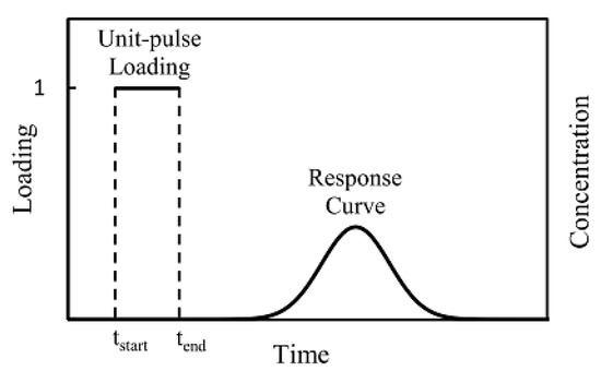
Figure 2.
Schematic representation of unit-pulse loading and response curve [50].
2.5. Optimization Inverse Problem in Integrated Aquifer-River Domain
Equations (7) and (20) should be solved simultaneously in an integrated aquifer-river domain, to compute the groundwater contaminant source release histories with the use of known measured concentrations in the river. This is an inverse problem and since the number of equations and the number of unknowns are not equal, the system is over-determined that requires a special technique to be solved. The optimization technique is a widespread tool in solving these problems. Fmincon solver, available in the optimization toolbox of MATLAB R2017b software [65], is one of the classic optimization methods to solve the constrained minimization problems that can be employed in the present research. It uses different search algorithms to find the optimal point of a constrained linear/nonlinear multivariable function. In this work, the Interior point algorithm of the Fmincon solver is used; it solves linear and nonlinear convex optimization problems.
The optimization solution starts with an initial guess (w0) as an unknown input vector value (source release histories) and the convergence of Karush-Kuhn-Tucker () conditions is checked. The approach minimizes the objective function objF in Equation (23) considering upper and lower constraints on pollutant release history (w):
where m is the number of concentration observations, Ci represents the measured concentration in the river downstream, the estimated concentration in the river downstream using the forward model and wmax are upper values of injected source fluxes in groundwater model. If the constraints are satisfied, the optimal solution has been reached, otherwise, the algorithm moves to a new point changing the search direction utilizing the Newton-Raphson method, and changing the step size (applying the merit function or the filter methods) to obtain an updated estimation. These steps will continue until the convergence criterion is achieved. For more details, see [66].
2.6. Error on Observations
In real field cases, due to the limited precision of the measurement devices and the influence of sampling conditions, errors may be developed in the measured data. So, in the synthetic scenarios, to evaluate the performance of simulation–optimization methodology in the presence of measurement errors, we resort to corrupt the sampled true concentration data by adding random relative errors according to the following relationship [67]:
where is a random number from a Gaussian standard population, stands for the error amplitude and the product is equal to the relative measurement error in the generic location . Normal random errors equal to 5% and 10% of the standard deviation have been applied in the present study. It should be noted that one set of concentration data perturbed by Equation (24) corresponds to one sample realization. By generating corrupted observations, it is possible to evaluate the performance of the proposed model for different sample realizations and to obtain an average result together with an estimate of the outcome uncertainty [30]. In this work, 10 different realizations have been considered.
2.7. Evaluation of Performance
Since the problems in hand are synthetic cases, the outcomes are compared with the actual contaminant release histories and the estimated data. The results are evaluated according to the metrics used by Ayvaz [30]: normalized error (NE), percent average estimation error (PAEE), standard deviation (SD), Equation (25) and with the known metrics proposed by Anderson and Woessner [68], Equation (26): mean error (ME), mean absolute error (MAE), root mean squared error (RMSE) and normalized root mean squared error (NRMSE).
where is the average (on realizations) computed flux for the stress period and source and is the actual source fluxes for the same period and source.
3. Results and Discussion
Two case studies with different scenarios have been considered to verify the methodology. The first is a literature test case [30,48] dealing with groundwater pollution, and the second is a new case, never introduced before, which considers groundwater–river integrated system and analyzes the groundwater contamination, originating from leakage from an underground damaged tank, as moving to the river and then traveling downstream along the watercourse.
3.1. First Case Study—Literature Case Study
To evaluate the applicability of the proposed methodology, we considered a literature case introduced by Ayvaz [30] and later adopted in Xing et al. [48]. Figure 3 shows the discretization grid of the numerical model of the studied aquifer. Table 2 summarizes the hydraulic and geometry characteristics. For this aquifer, the specified head boundary conditions on the upper-left () and lower right () side, and no-flow boundary at the other sides are considered. The head values on the and sides are 100.0 m and 80.0 m, respectively above a horizontal plane. The aquifer system consists of five different hydraulic conductivity zones, whose isotropic conductivity values are: = 0.0004 m/s, = 0.0002 m/s, = 0.0001 m/s, = 0.0003 m/s and = 0.0007 m/s. The conductivity values are taken as uniform inside each zone. Therefore, the aquifer case dealt with a steady-state and non-uniform flow conditions one. There are two active contaminant sources ( and ) and seven monitoring locations (–) in the aquifer domain. The total simulation time is 10 years divided into 20 stress periods () of 6 months each. It is assumed that both sources release conservative compounds during the first 24 months. Therefore, the contaminant transport process in the aquifer is transient.
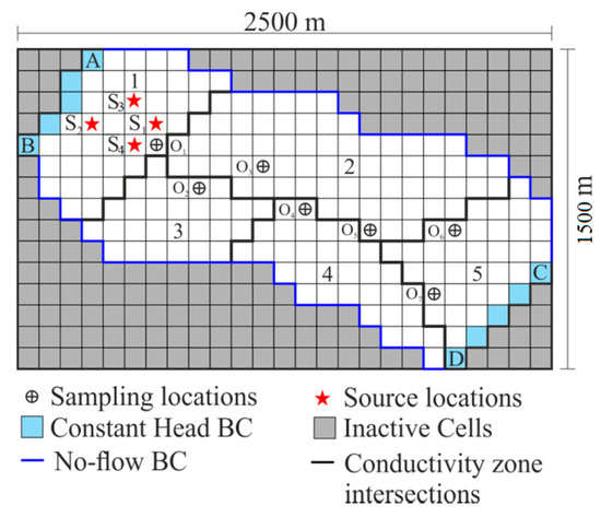
Figure 3.
Two-dimensional aquifer model.

Table 2.
Case 1: hydraulic and geometry characteristics.
3.1.1. Procedure to Estimate the Contaminant Release History in the Aquifer
Since it is a hypothetical case study, observed data generation is required. To achieve this goal, a forward model including flow and contaminant transport models is employed. The following main steps are needed to be followed:
- Setting up a groundwater flow and transport numerical model of the case study. The MODFLOW [69] and MT3DMS [70] codes are used for this purpose. In this process, the domain of the solution is a network with block-centered grids where the values of the piezometric heads, the velocities and contaminant concentrations in the center of cells are computed;
- Injecting the true release contaminant at the source and recording the concentration data in the monitoring points as ;
- Applying the unit loadings in each source separately and calculating the breakthrough curves at the monitoring locations;
- Computing the transfer functions () by processing the observed breakthrough curves;
- Solving the optimization problem [Equation (23)] to identify the unknown release history that best fits the estimated data to the observed ones.
3.1.2. Results
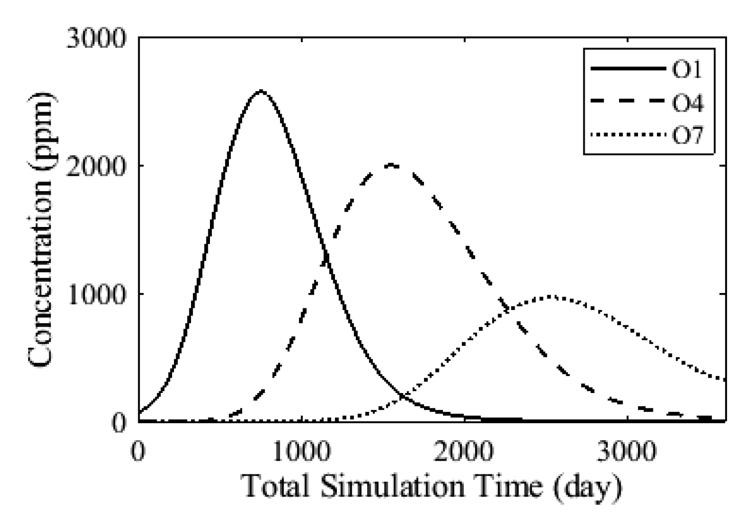
MODFLOW and MT3DMS codes are applied to simulate the groundwater flow and transport processes, respectively; the concentration data in monitoring wells are extracted from the results and adopted as observations. Few concentration curves in sampling wells , and are shown in Figure 4 as an example. The transfer functions (g(x,t) of Equation (5)) at the end of the simulation are presented in Figure 5 for both sources and seven specified sampling wells. For the present case, several scenarios to identify sources release histories are considered; in all of them, the observed concentration-time series at monitoring wells are considered as input data for the inverse problem. Some analyzed scenarios have been introduced by Ayvaz [30].

Figure 4.
Concentration curves in the sampling locations
, and .

Figure 5.
Transfer function curves in sampling wells due to source 1 (a) and source 2 (b); they represent g(x,t) of Equation (5).
- First scenario
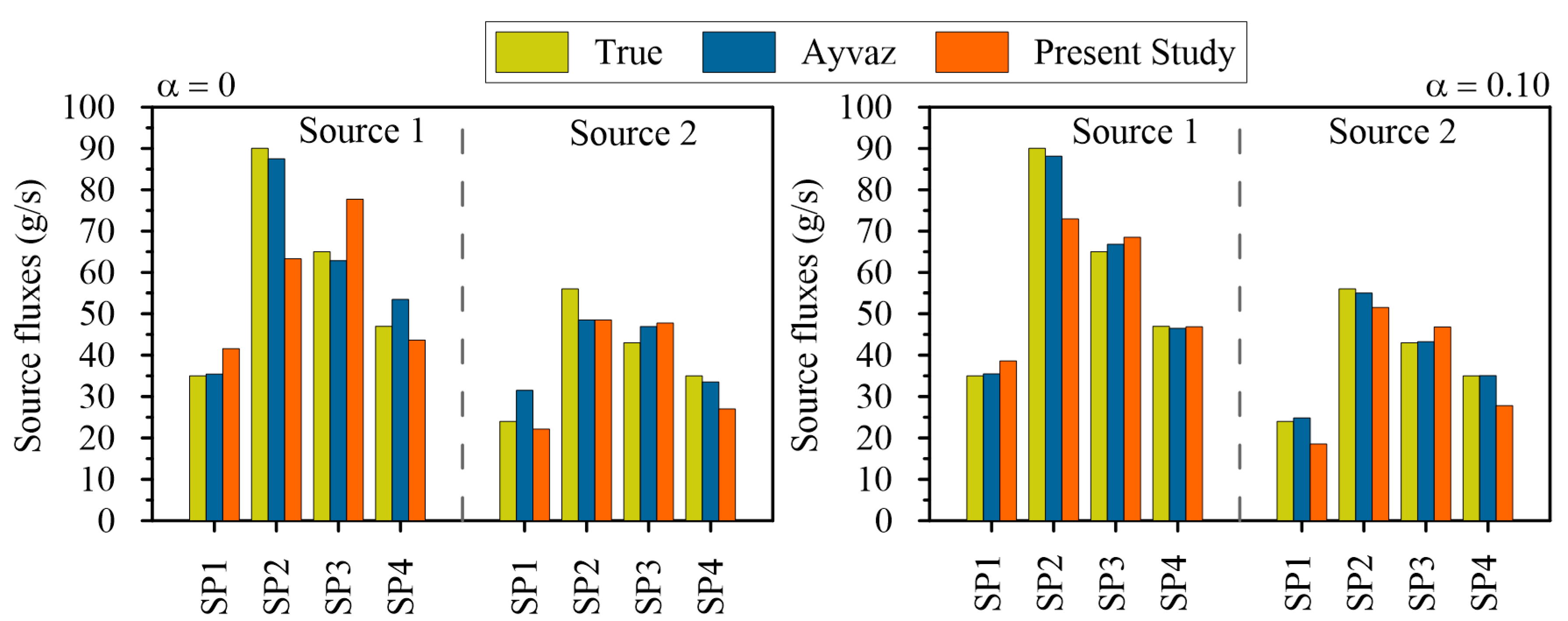
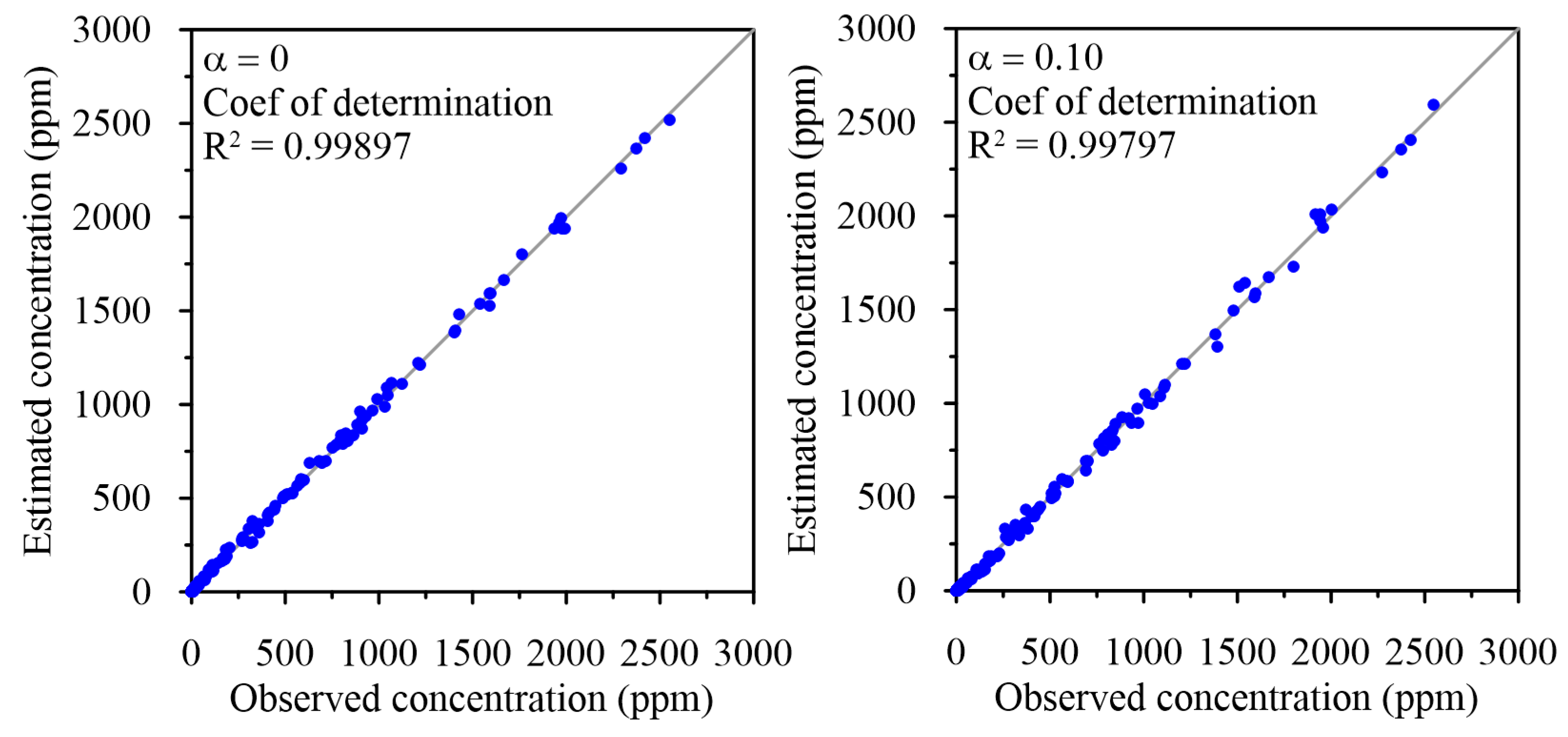
In this scenario, the purpose is the identification of sources release histories ( and ) using the transfer function theory, assuming that the source locations are known. It is also assumed that the concentration data are available only at the end of each stress period with a length of 180 days. Therefore, taking into account 20 stress periods and seven monitoring wells, 140 concentration data are recorded as observations. Finally, the release histories of the two sources were recovered. Figure 6 shows the results of the identification of the release histories. The results are compared with those of Ayvaz [30] in two cases, error-free and perturbed data. The estimated versus observed concentrations are presented in Figure 7; it is clear that the approach estimated well the concentration observations. Ayvaz [30] applied his model for simultaneous identification of unknown locations and release histories of the groundwater contaminant sources. For more details, see reference [30], where the total number of iterations of the identification process was 32,659, using the genetic algorithm (GA). The present approach, which is based on the transfer function theory, has the advantage of identifying release histories of sources with only one run of the simulation model. The resulting transfer matrixes are integrated with an optimization algorithm (Interior point algorithm of Matlab Fmincon solver) that converges to the specified tolerance in less than 600 iterations. The present methodology can identify source release fluxes, mostly with the same accuracy of the literature studies, employing only one run of the complete simulation model and in much less computation time: in fact, each application of the transfer function to surrogate the transport process requires only 1/100 of the computation time of the complete simulation model.

Figure 6.
Recovered release histories of sources 1 and 2 in error-free data condition (α = 0) and in error-perturbed data condition (α = 0.1).
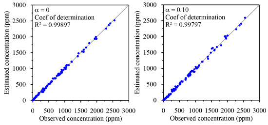
Figure 7.
Estimated vs. observed concentration in error-free data condition (α = 0) and in error-perturbed data condition (α = 0.10).
The present approach outcomes are compared with the ones obtained by [30] in Table 3. Although applying of 10% error to concentration data the results show some differences when compared to [30] considering PAEE, it can be noted that the present methodology produces even better results than [30] in identifying source fluxes in some stress periods. Furthermore, the results of the inverse solution have been achieved only with one simulation model run in much less computation time. This significant advantage justifies the application of the present approach in real and complex cases, when large inverse problem dimensions are involved.

Table 3.
Comparison of the estimated and actual source release histories with Ayvaz (2010) in α = 0.1.
Table 4 reports, according to Equation (26), the computed ME, MAE, RMSE and NRMSE for the source fluxes for all the studied scenarios in the present work. Regarding the first scenario, the present approach can well reproduce the source fluxes even if Ayvaz performs better. This is due to the approximation of using the transfer function instead of the full model and to the minimization algorithm.

Table 4.
Mean error (ME), mean absolute error (MAE), root mean square error (RMSE) and normalized root mean squared error (NRMSE), computed for case study 1 on source fluxes (g/s).
Several case studies, not reported here for brevity, to identify contaminant source release histories have been performed; increasing the number of contaminant sources, changing the monitoring locations and scenarios to determine the minimum number of sampling locations. In the end, the most important result is that, if the number of contaminant sources increases, the number and location of the monitoring wells and their distance from the contaminant sources become crucial in the identification of contaminant source release histories. Increasing the number of contaminant sources, the number of unknown variables in the optimization problem increase and for recovering the characteristics of the sources, more information about the contaminant sources is needed. This information can be obtained from the sampling points which contain information on the distribution of contamination concentrations at different times. The position of sampling points is another important issue that needed to be considered. The closer points to the source are important in retrieving the contaminant source values in the initial times, where for the far ones are effective in retrieving the contaminant source values in the succedent time of a mass loading pattern. Additionally, recovering two or more sources using only one measurement point is impossible, due to the non-uniqueness difficulty. In this case, the effect of the sources is convoluted, and an infinite number of solutions can be found. On the other hand, placing a large number of monitoring points would also result in redundancy in the information collected. Therefore, an appropriate monitoring network design, which can provide sufficient information related to the distribution of contamination, is strongly recommended in real field cases.
It is interesting to know what the results will be if the new goal is to identify the source fluxes for all simulation periods, and not only for the first 2 years. In other words, is the present methodology, based on transfer function theory, capable to identify source fluxes accurately if there is no information about the time starting of the release? The second scenario was developed to investigate this question.
- Second scenario
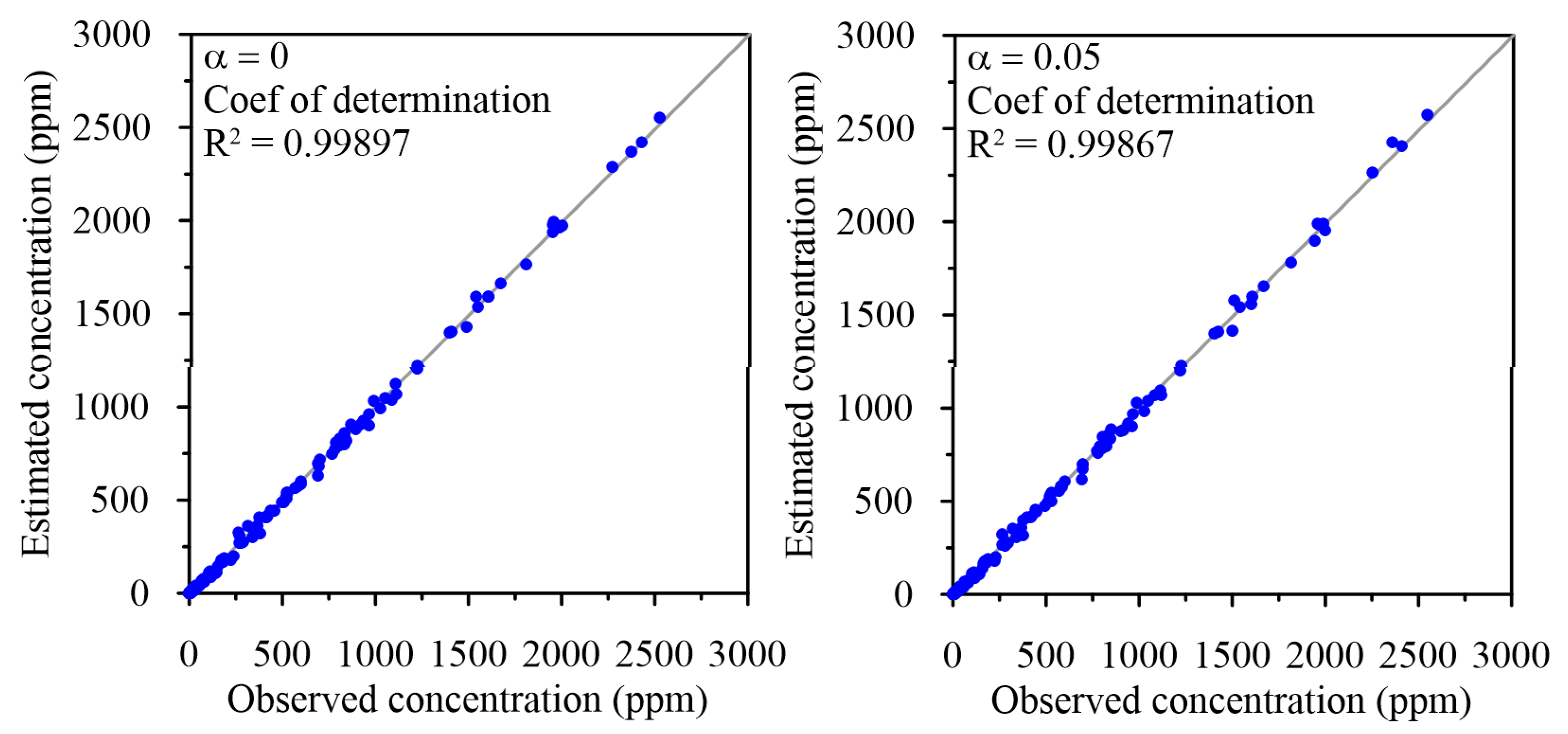
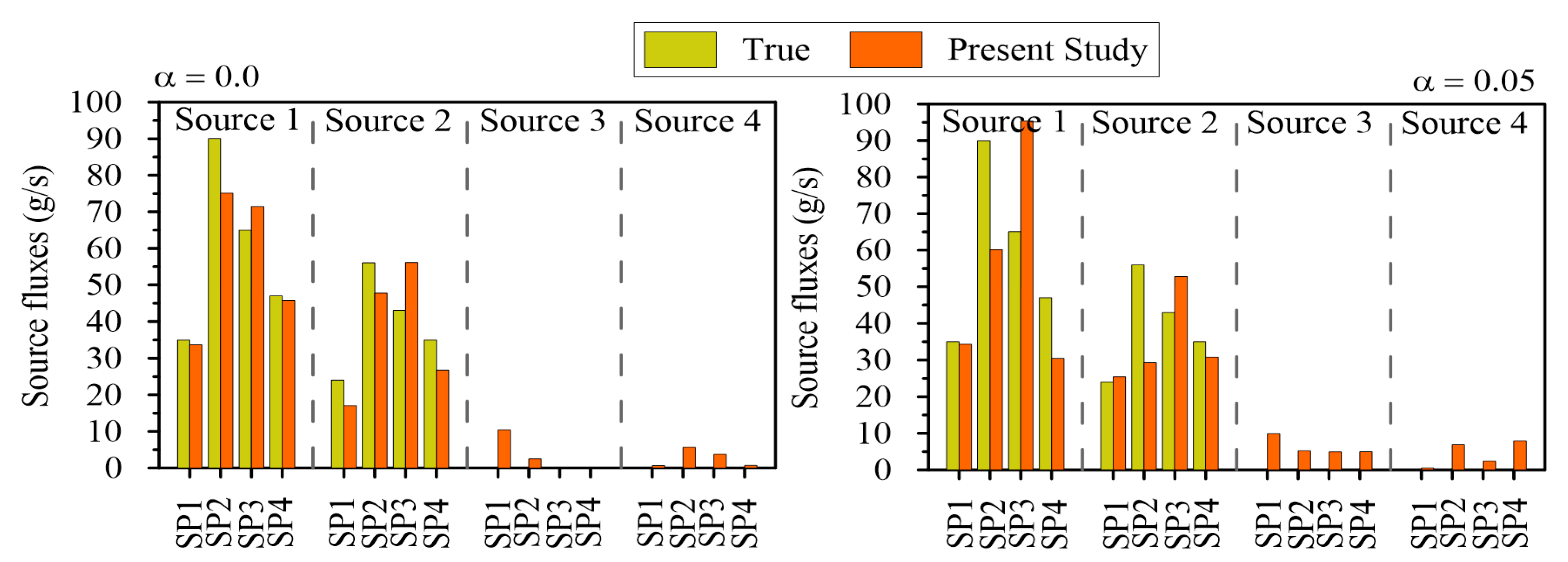
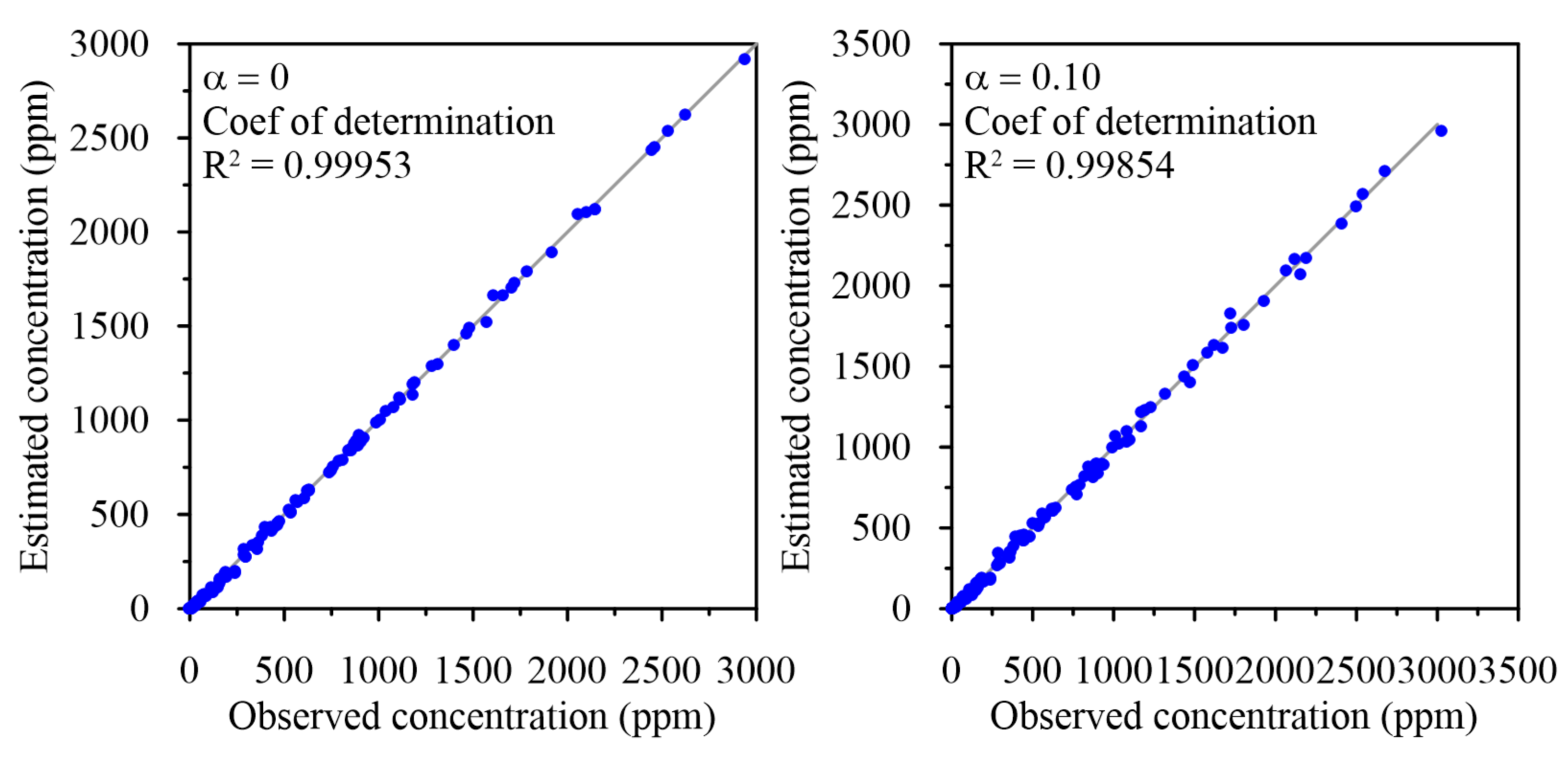
In this scenario, a set up to identify the source release histories for 10-years simulation periods (3600 days) with a stress period of 180 days is prepared. Considering two sources S1 and S2 with the same number of observations used in the first scenario, 40 unknown release fluxes will be detected. An error level of 5 % is applied to the observation and 10 realizations are generated. Figure 8 shows the results of source fluxes identification in error-free and error-perturbed data conditions. Estimated versus observed concentrations are also presented in Figure 9. Additionally, in this scenario, the method estimates very well the concentration observations.
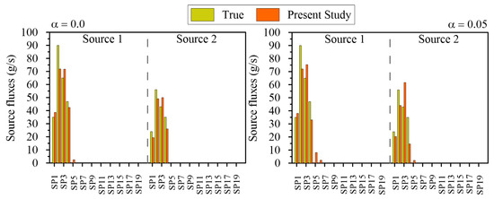
Figure 8.
Recovered release histories of sources 1 and 2 in error-free data condition (α = 0) and in error-perturbed data condition (α = 0.05).
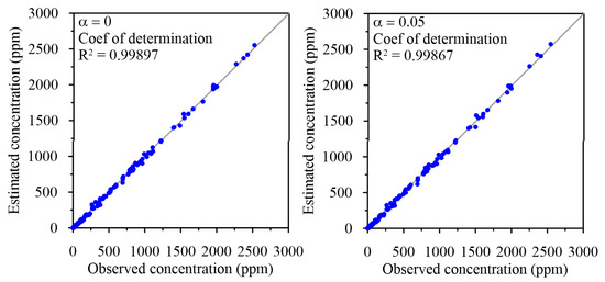
Figure 9.
Estimated vs. observed concentration in error-free data condition (α = 0) and in error-perturbed data condition (α = 0.05).
For this case, see Table 4, the calculated NRMSE was 4.3% and 7.1 % in error-free and error-perturbed data conditions, respectively. These results show that the presented methodology can identify source release history properly, considering the same number of observations of the first scenario and no information about the starting or ending time of the source activity.
- Third scenario
For a more accurate comparison with [30], the locations of sources are assumed to be unknown. In this regard, the approach proposed by [17] is used, which assumes the existence of several potential sources in the domain. The locations of the sources should be introduced to the model. If the location of a source is not known, a candidate location or locations can be introduced to the model as potential sources. The model will obtain the release history of all introduced sources. The location with a remarkable release history represents a true source and the location with release history close to o zero is a false one. According to that, four contaminant possible sources (sources 1 and 2 are real source locations; sources 3 and 4 are potential sources) are hypothesized in the aquifer, see Figure 3. The transfer function curves of the seven monitoring wells resulting from sources 1 and 2 are the same (see Figure 5a,b), and the ones from the sources 3 and 4 are depicted in Figure 10a,b, respectively.

Figure 10.
General transfer function curves in seven sampling wells due to source 3 (a) and source 4 (b); they represent g(x,t) of Equation (5).
Considering the same observation used in the two previous scenarios, the reconstructed release histories are obtained and presented, for error-free and error-perturbed data conditions, in Figure 11. The method estimated the source release history at all four potential sources. It is clear, from Figure 11, that, although some negligible concentration values were estimated for the release histories at the sources 3 and 4, the present model correctly identifies the real sources 1 and 2. Sources 3 and 4 are false, due to the close to zero release history. This demonstrates the capability of the model, not only in the source release estimation, but also in its location identification. Calculated NRMSE is equal to 7.8% and 15.7% in free-error and error-perturbed data conditions, respectively. It can be concluded here that the present methodology can efficiently identify the release histories, even when the source locations are unknown and the observed concentration data are not accurate with only one run of the complete simulation model. Each application of the transfer function to surrogate the transport process requires only 1/100 of the computation time of the complete simulation model. The estimated versus observed concentration data curve in the free-error scenario and for 10 realizations of error-perturbed data conditions are shown in Figure 12. The method estimates well the concentration observations.

Figure 11.
Recovered release histories of sources 1, 2, 3 and 4 in error-free data condition (α = 0) and in error-perturbed data condition (α = 0.05).
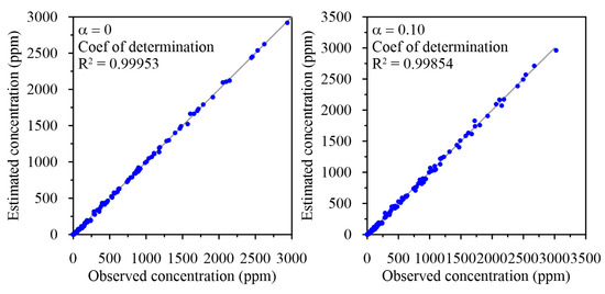
Figure 12.
Estimated vs. observed concentration in error-free data condition (α = 0) and in error-perturbed data condition (α = 0.1).
3.2. Second Case Study—A Groundwater-River Integrated System
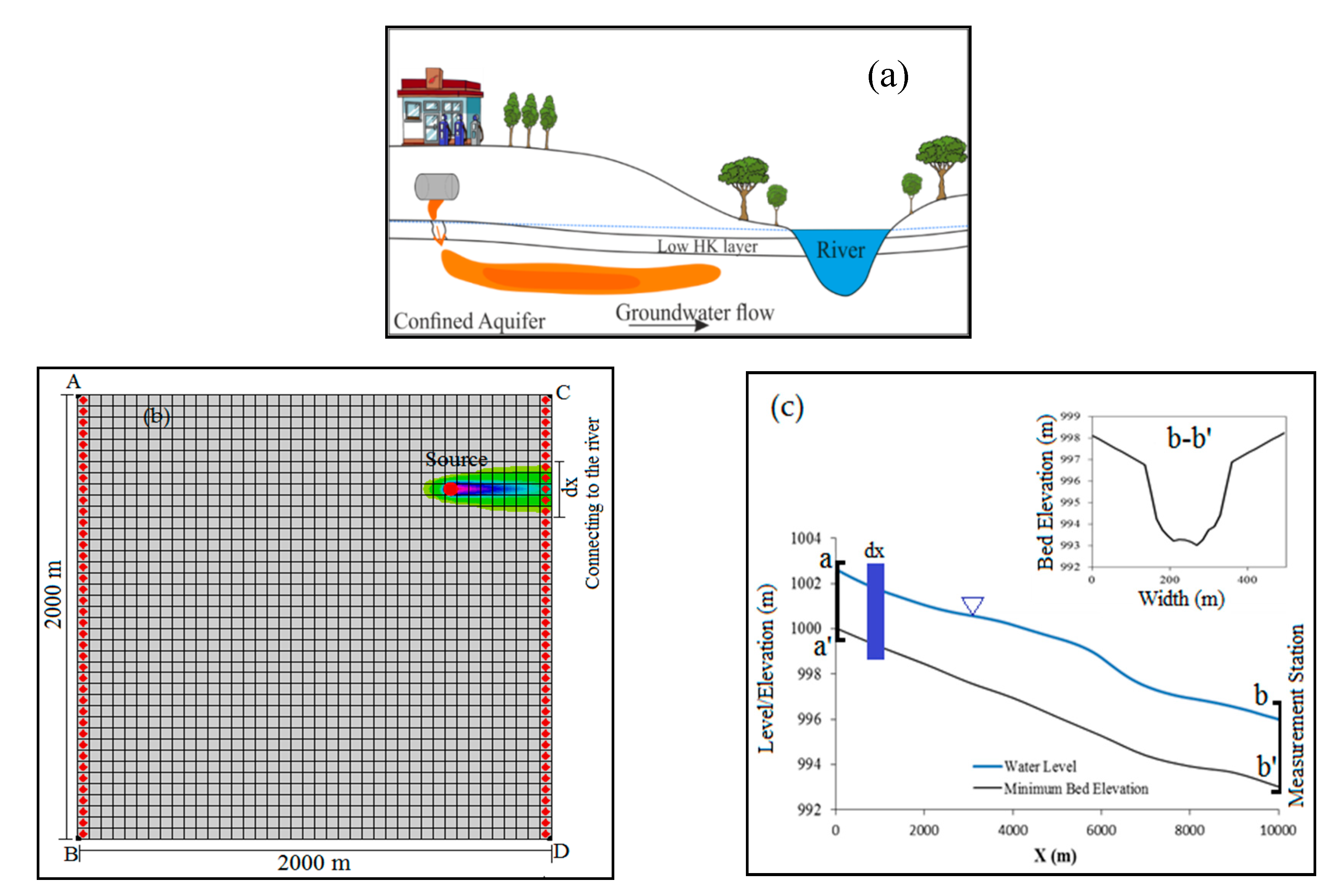
The second test case deals with a hypothetical transport of a conservative pollutant that is released in a confined aquifer and reaches a river, then moves along the stream to a monitoring cross-section where it is detected. The pollution origin is spilling from an underground tank that reaches the confined aquifer below through a discontinuity in the top confinement (see Figure 13a for a sketch view). The contaminant then moves into the groundwater body reaching the downstream river.
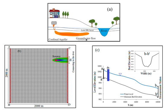
Figure 13.
(a) Sketch view of the case study; (b) the plan view of the study area and the distribution of contaminant source after 182 days; (c) water surface profile in the river and cross-section at the chainage 10 km.
The confined 2-D aquifer has dimensions 2000 m × 2000 m (Figure 13b). The saturated thickness of the aquifer varies from 58.75 m to 10 m from west to east side. This thickness decreases due to the rising of the aquifer bottom (1.5%) and a lowering of the top boundary (1%). The north and south sides (AC and BD) have no-flow boundary conditions and the west one (AB) has a specified head. The east boundary is contiguous to the river. The boundary condition on the east side (CD) is coherent with the river water levels that have been extracted from the results of the flow simulation model. The head value on the boundary AB is 1022.0 m above a horizontal reference plane; the hydraulic conductivities are anisotropic with values in x and y directions = 0.0007 m/s and = 6.95·10−5 m/s, respectively. Steady-state and uniform flow conditions in the aquifer are assumed. One active contaminant source in the aquifer and one measuring location in the river downstream are considered. The total simulation time is 1 year divided into four stress periods (SP) of 3 months equal duration. It is assumed that the source releases a conservative compound with unit discharge during each stress period. Thus, the contaminant transport process in the integrated aquifer-river system is transient. The values of the hydrogeological parameters are given in Table 5 (x and y coordinates are oriented to east and north directions, respectively). It has to be noticed that, for a source with unit volumetric discharge, the source mass loading (W) is equal to the concentration (C), because of the equation W = Q · C.

Table 5.
Case 2: hydraulic and geometry characteristics.
The synthetic river is 10 km long with 11 irregular cross-sections 1 km apart. Flow depth and discharge results are distributed along the stream in 101 and 100 intervals, respectively. Constant discharge of 300 m3/s with a contaminant concentration equals to zero is considered as a boundary condition on (). A constant water level of 996 m and zero concentration gradient are regarded on () as boundary conditions. Figure 13c shows the water level profile and the cross-section at the chainage 10 km. The concentration-time data, resulting from the simulation at the chainage 10,000 m, are considered as observations in the virtual experiment. These observations have been used to estimate the release history in the point source located in the aquifer by the developed method.
It is considered, for sake of simplicity, a conservative contaminant; but it is important to note that the transfer function approach can be applied also for sorbing reactive solute [18].
3.2.1. Procedure to Estimate Contaminant Release in Aquifer-River Domain
In the integrated aquifer-river system inverse problem, the purpose is the identification of the groundwater contaminant source release histories using the known measured concentrations in the river. Therefore, Equations (7) and (20) should be solved simultaneously. The following are the main steps in solving the inverse problem:
- Setting up the river forward hydrodynamic model using MIKE11;
- Identification of the specified extension of the river connected to the aquifer;,extraction of the water levels in the river model and inserting them as the hydraulic boundary conditions of the aquifer model;
- Setting up a groundwater flow and transport model considering known release history () in the contaminant source by the MODFLOW and MT3DMS codes;
- Computing the concentrations in the cells at the intersection with the river and simulation of the contaminant transport process in the river by MIKE11 to obtain in the control section of the river downstream;
- Computing the in the intersection cells and the in the control section of the river downstream using the unit loading method;
- Computing the vector in Equation (7) considering the known vector and the matrix ;
- Converting to the mass loading vector by the relation , where is the groundwater discharge from the aquifer to the river in each cell, then applying as transport boundary conditions in the river model;
- Computing (equal to in the control section of the river downstream) in Equation (20), considering the known vector and the matrix ;
- Solving the optimization problem (Equation (23) to identify the unknown contaminant source release history, which results in best fits the observed data compared to the estimated ones.
3.2.2. Considerations at the Intersection of the Integrated Aquifer-River System
- The flow direction
Groundwater flows naturally in the gradient direction. In areas where groundwater levels are below the river water surface system, the direction of groundwater flow will be from the river to the groundwater system. Streams that receive water from the groundwater system are called ‘gaining’ streams and those that lose water to the groundwater system are called ‘losing’ streams. The gaining or losing character of streamflow may be consistent throughout a stream or it may be highly variable based on the stream reach location. The flow direction at the aquifer-river intersection is regarded from the groundwater into the river (gaining stream).
- Source type
Let us consider the rectangular area of the cells of the aquifer discretized domain located on the integrated border with dimension and in and directions, respectively. The boundary condition at the aquifer-river intersection is considered as a distributed source. Butera and Tanda [66] showed that the influence of and is remarkable only if the source dimensions are comparable to the plume extension. Therefore, considering the definition of point source “point source is a source with negligible area compared to where it drains’’ [71], and the insignificant dimensions of distributed sources applied in the present research, Equation (17), which is valid for the point sources, can be used to compute in the river downstream cross-section.
- Time scale
Generally, since the movement of groundwater is much slower than the one of the rivers, the time scale of the transport process in the groundwater and river is month/year and hour/day, respectively. On the other hand, in an integrated aquifer-river system, the time scale of the groundwater simulation model affects the time scale of the river transport process. It means that if the total simulation time in the groundwater model is, for example, one year, the simulation time in the river model needs to be also one year. This makes the task difficult to handle in terms of calculating the transfer function in the river model. In fact, the yearly computation of the transfer function in the river requires storing the concentration data with a small-time discretization that would lengthen the computation time. Considering large time discretization reduces the computation time and on the other hand, leads to a loss of concentration information to form the transfer matrix. Accordingly, the river transfer function is computed for one day considering a small-time discretization to keep the concentration information. Then, assuming the system characteristics are constant over time, the transfer function is extended for the entire simulation period. It is important to remark that the river flow is assumed in steady state.
3.2.3. Results
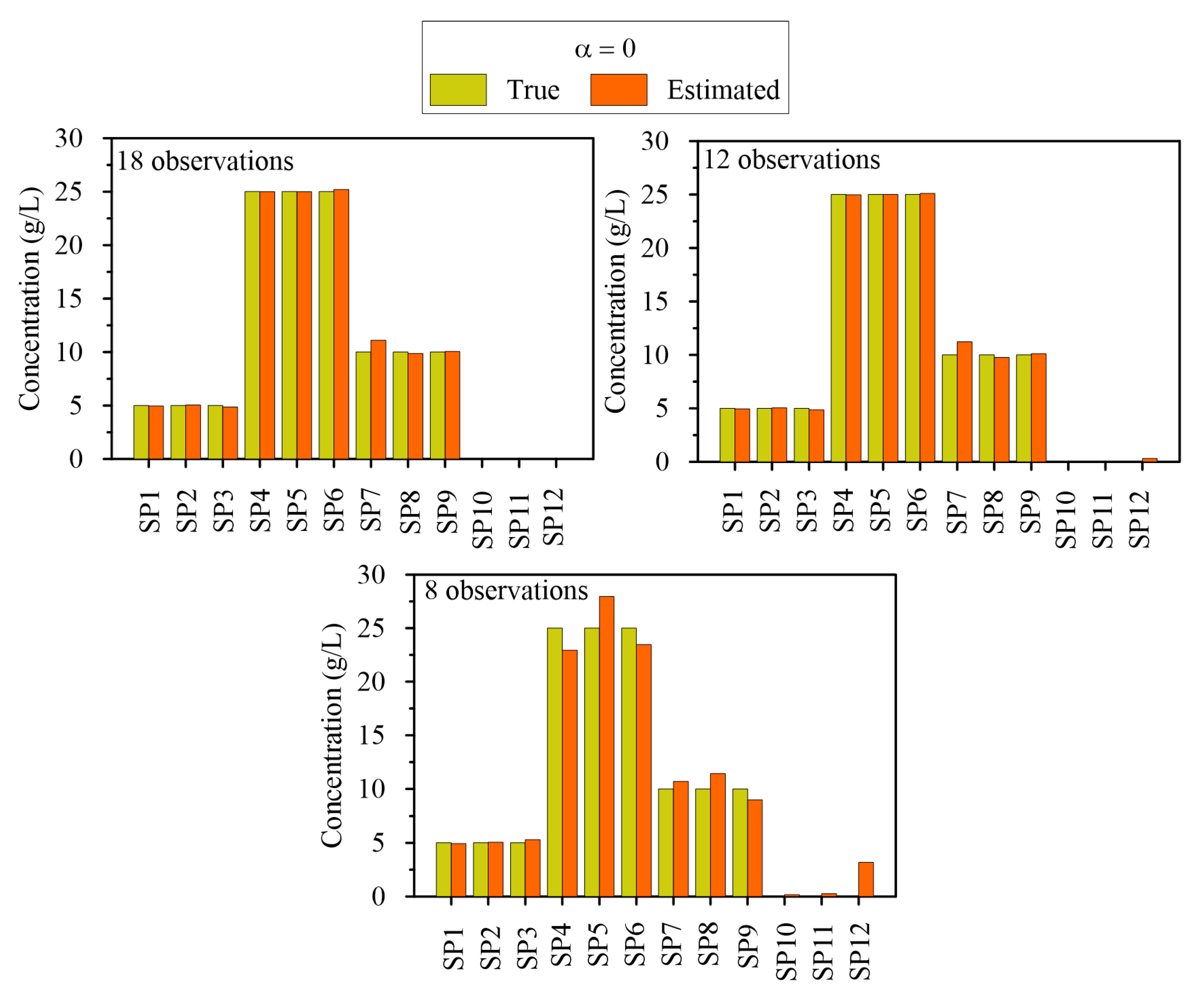
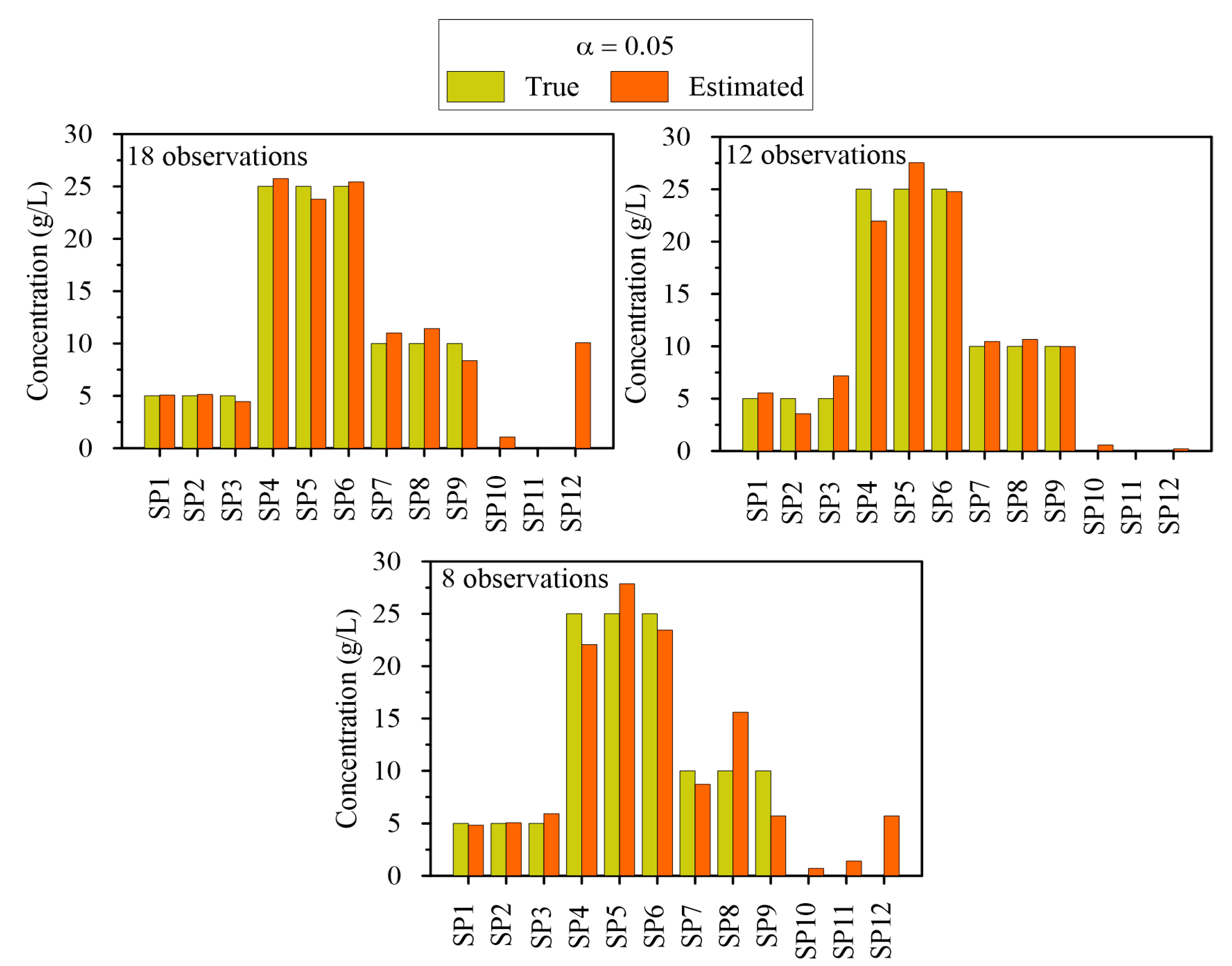
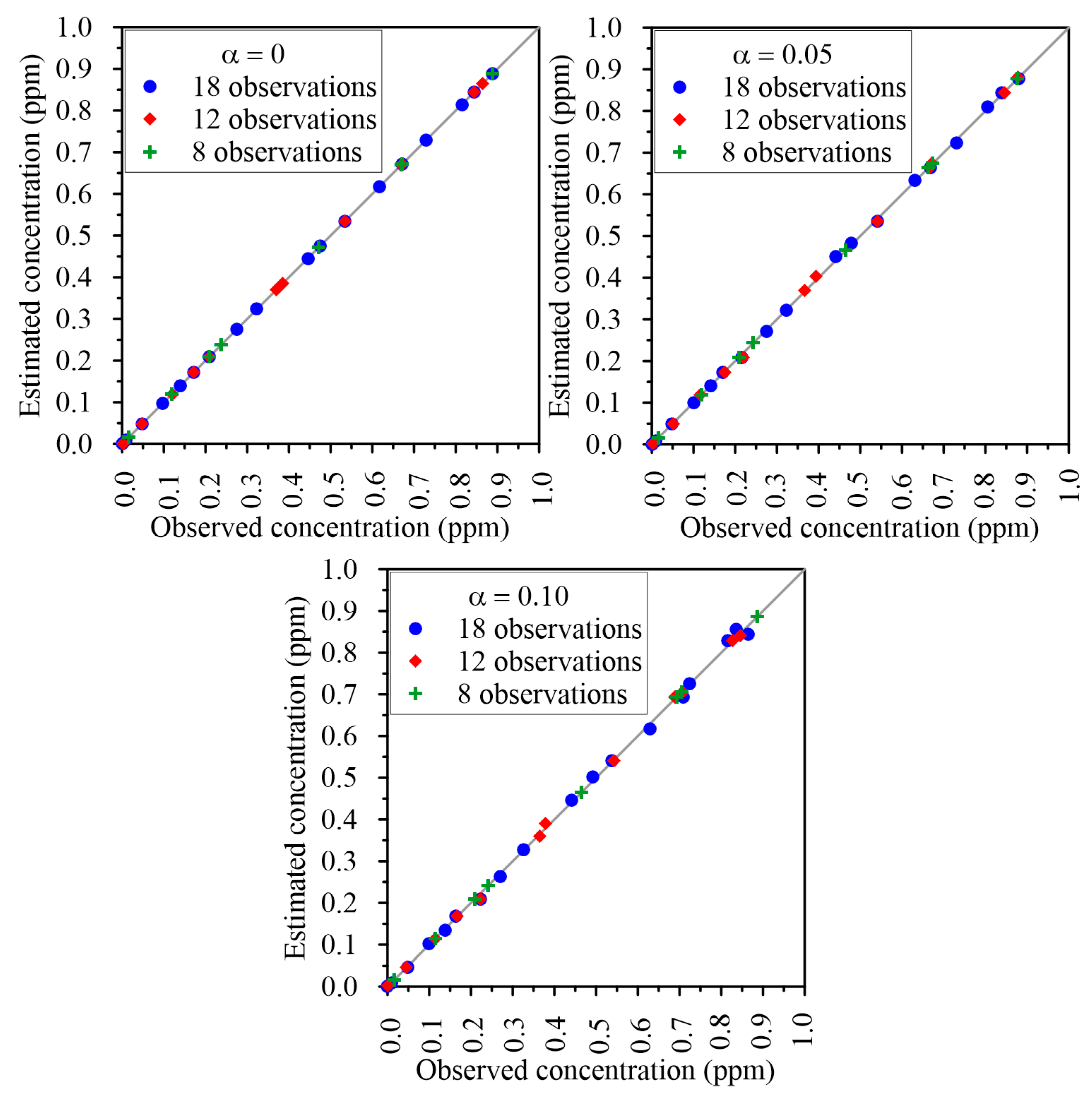
The contaminant is released in the aquifer at the known source of Figure 13b; then, the groundwater flow moves the contaminant to the river and the river, in turn, transports the contaminant downstream. Concentrations at chainage 10,000 m are recorded during the model simulation and used as observations to recover the release history in the aquifer. Various scenarios of source release histories identification are considered which includes different cases of data availability (8, 12, and 18 observations), applying error to the data with different noise levels (error-free, α = 0.05, α = 0.10), and unavailability of information about the length of the stress periods. For all scenarios, the release histories are estimated for each month. In the first scenario, the observed concentration data are available every 20 days. Therefore, for the total simulation time equal to 1 year, 18 data, as observed concentration data, are considered. To get closer to realistic conditions, the second and third scenarios are also carried out assuming observed concentration data available only at the end of each month (12 observations) and every 45 days (eight observations), respectively. Release histories recovery resulted in an error-free and error-perturbed data conditions for a considered point source in the homogeneous aquifer are presented in Figure 14, Figure 15 and Figure 16. The estimated versus observed concentration data and statistical parameters showing the capability of the model accuracy to estimate source release histories are provided in Figure 17 and Table 6, respectively. It is clear, from Figure 17, that the approach can reproduce the observed concentrations for all nine studied cases.
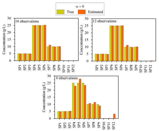
Figure 14.
Source release histories in error-free data condition (α = 0) with 18, 12 and 8 observed concentrations data.
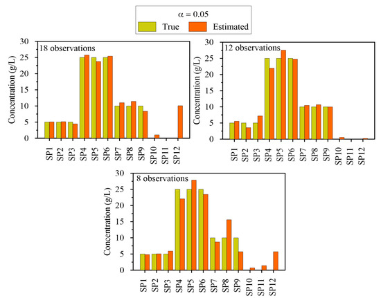
Figure 15.
Source release histories in error-perturbed data condition (α = 0.05) concentration with 18, 12 and 8 observed concentrations data.
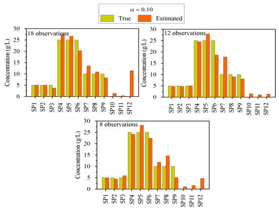
Figure 16.
Source release histories in error-perturbed data condition (α = 0.1) with 18, 12 and 8 observed concentrations data.
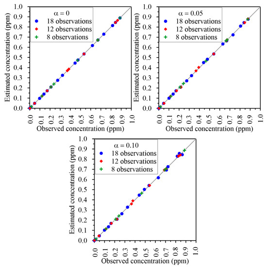
Figure 17.
Estimated vs. observed concentration in the various scenarios.

Table 6.
Statistical parameters to test the accuracy in estimation of the source release histories.
It should be noted, from Table 6 that, in error-free data condition, due to the existence of more contaminant plume information, increasing the numbers of observed concentration data caused the normalized root mean squared error to decrease. It can also be seen that by applying error perturbed data, the of the source identification model shows higher magnitudes than the error-free data scenario ones. By comparing the results in the two noise levels of 5% and 10 %, as expected, the results obtained with a greater error show higher value.
Considering the statistical parameters reported in Table 6, the scenario with 12 observations is the best one to identify sources release histories. In this study case, one can observe that it is unexpected because, with the increasing number of observations to 18, the model should perform more efficiently in the source identification process. This can be explained considering that not only the number of observed data but also the times at which concentration data are observed are significant. Thus, considering that the process of applying error is completely random, increasing the number of data to 18 may not lead to better results in terms of identifying source release histories. The analysis of Figure 14, Figure 15 and Figure 16 show that the present simulation–optimization approach can efficiently identify source release histories in the aquifer–river integrated systems, even when inaccurate observed concentrations data are provided. Finally, comparing Figure 14, Figure 15 and Figure 16, it is possible to see the influence of the error on observations on the recovery of the release history.
4. Conclusions
A simulation–optimization approach dealing with the identification of the contaminant source characteristics in groundwater and groundwater-river integrated systems has been presented in this study. To reduce the forward model computation time and makes it practical, the transfer function theory is applied as a surrogate model and integrated with an optimization algorithm (interior point algorithm of Matlab Fmincon solver) to estimate the contaminant source characteristics within the process of groundwater and river mass transfer simulation.
Two main case studies and scenarios are considered for the performance evaluation of the proposed model. The first one is a heterogeneous aquifer, which was well-known and chosen in many studies in the literature. Some scenarios reproduce sources release histories already tested in the literature. The results show the surrogate model based on the transfer function theory remarkably reduces computational time, and can well recover the characteristics of contaminant sources (source release histories and locations). The second case is a hypothetical aquifer-river system never investigated before. The main objective of this application is the identification of the release history, originated from a groundwater contaminant source, using observations recorded downstream in the river. The results, analyzed with well-known metrics, show the simulation–optimization approach used in this study can also satisfactorily identify the source release history, even with inaccurate observed concentration data.
The transfer function theory is shown as an efficient approach to create a surrogate transport model for reducing the computational time of the simulation model. It should be noted that the crucial phase of the developed method is the definition of an accurate transfer function, which, in turn, can lead to a robust and effective solution process. In fact, in some cases, it is not possible to compute an excellent transfer function due to the complex boundary conditions and parameters that govern the system. Moreover, it has to be pointed out that the transfer function can be defined for linear problems only. For this reason, there still a remarkable area to conduct further research to provide comprehensive instructions for using the transfer function theory in groundwater and surface water problems including multiple sources.
Supplementary Materials
The following are available online at https://www.mdpi.com/2073-4441/12/9/2415/s1, list of symbols.
Author Contributions
Conceptualization, J.M.V.S., H.M.V.S., A.Z. and M.M.; Methodology, A.J., J.M.V.S., H.M.V.S., A.Z., M.G.T. and M.M.; Software, A.J.; Supervision, J.M.V.S., H.M.V.S., A.Z., M.G.T. and M.M.; Validation, A.J., J.M.V.S., A.Z. and M.G.T.; Visualization, A.J., J.M.V.S., H.M.V.S., A.Z., M.G.T. and M.M.; Writing—Original draft, A.J.; Writing—Review & editing, A.J., J.M.V.S., H.M.V.S., A.Z., M.G.T. and M.M. All authors have read and agreed to the published version of the manuscript.
Funding
This study is part of a Ph.D. thesis at Tarbiat Modares University which was funded by the Ministry of Science Research and Technology of Iran (MSRT) for the cooperation with the Department of Engineering and Architecture of the University of Parma (Italy).
Acknowledgments
Azade Jamshidi, Jamal Mohammad Vali Samani, Hossein Mohammad Vali Samani, and Mehdi Mazaheri thank M.S.R.T. for their support of the present research. We thank three anonymous reviewers for their valuable comments and suggestions.
Conflicts of Interest
The authors declare no conflict of interest.
References
- Zanini, A.; Woodbury, A.D. Contaminant source reconstruction by empirical Bayes and Akaike’s Bayesian Information Criterion. J. Contam. Hydrol. 2016, 185–186, 74–86. [Google Scholar] [CrossRef] [PubMed]
- Mazaheri, M.; Mohammad Vali Samani, J.; Samani, H.M.V. Mathematical Model for Pollution Source Identification in Rivers. Environ. Forensics 2015, 16, 310–321. [Google Scholar] [CrossRef]
- Skaggs, T.H.; Kabala, Z.J. Recovering the release history of a groundwater contaminant. Water Resour. Res. 1994, 30, 71–79. [Google Scholar] [CrossRef]
- Lattés, R.; Lions, J.L. The Method of Quasi-Reversibility, Applications to Partial Differential Equations; Elsevier: New York, NY, USA, 1969. [Google Scholar]
- Liu, C.; Ball, W.P. Application of inverse methods to contaminant source identification from aquitard diffusion profiles at Dover AFB, Delaware. Water Resour. Res. 1999, 35, 1975–1985. [Google Scholar] [CrossRef]
- Bagtzoglou, A.C.; Dougherty, D.E.; Tompson, A.F.B. Application of particle methods to reliable identification of groundwater pollution sources. Water Resour. Manag. 1992, 6, 15–23. [Google Scholar] [CrossRef]
- Liu, J.; Wilson, J.L. Modeling travel time and source location probabilities in two-dimensional heterogeneous aquifer. In Proceedings of the 5th WERC Technology Development Conference, Las Cruces, New Mexico, 18–20 April 1995; pp. 59–76. [Google Scholar]
- Woodbury, A.D.; Ulrych, T.J. Minimum Relative Entropy Inversion: Theory and Application to Recovering the Release History of a Groundwater Contaminant. Water Resour. Res. 1996, 32, 2671–2681. [Google Scholar] [CrossRef]
- Cupola, F.; Tanda, M.G.; Zanini, A. Contaminant release history identification in 2-D heterogeneous aquifers through a minimum relative entropy approach. Springerplus 2015, 4, 656. [Google Scholar] [CrossRef]
- Neupauer, R.M.; Wilson, J.L. Adjoint method for obtaining backward-in-time location and travel time probabilities of a conservative groundwater contaminant. Water Resour. Res. 1999, 35, 3389–3398. [Google Scholar] [CrossRef]
- Neupauer, R.M.; Wilson, J.L. Adjoint-derived location and travel time probabilities for a multidimensional groundwater system. Water Resour. Res. 2001, 37, 1657–1668. [Google Scholar] [CrossRef]
- Neupauer, R.M.; Wilson, J.L. Backward location and travel time probabilities for a decaying contaminant in an aquifer. J. Contam. Hydrol. 2003, 66, 39–58. [Google Scholar] [CrossRef]
- Neupauer, R.M.; Borchers, B.; Wilson, J.L. Comparison of inverse methods for reconstructing the release history of a groundwater contamination source. Water Resour. Res. 2000, 36, 2469–2475. [Google Scholar] [CrossRef]
- Snodgrass, M.F.; Kitanidis, P.K. A geostatistical approach to contaminant source identification. Water Resour. Res. 1997, 33, 537–546. [Google Scholar] [CrossRef]
- Michalak, A.M.; Kitanidis, P.K. Estimation of historical groundwater contaminant distribution using the adjoint state method applied to geostatistical inverse modeling. Water Resour. Res. 2004, 40, W08302. [Google Scholar] [CrossRef]
- Boano, F.; Revelli, R.; Ridolfi, L. Source identification in river pollution problems: A geostatistical approach. Water Resour. Res. 2005, 41. [Google Scholar] [CrossRef]
- Butera, I.; Tanda, M.G.; Zanini, A. Simultaneous identification of the pollutant release history and the source location in groundwater by means of a geostatistical approach. Stoch. Environ. Res. Risk Assess. 2013, 27, 1269–1280. [Google Scholar] [CrossRef]
- Gzyl, G.; Zanini, A.; Frączek, R.; Kura, K. Contaminant source and release history identification in groundwater: A multi-step approach. J. Contam. Hydrol. 2014, 157, 59–72. [Google Scholar] [CrossRef]
- Cupola, F.; Tanda, M.G.; Zanini, A. Laboratory sandbox validation of pollutant source location methods. Stoch. Environ. Res. Risk Assess. 2015, 29, 169–182. [Google Scholar] [CrossRef]
- Chen, Z.; Gómez-Hernández, J.J.; Xu, T.; Zanini, A. Joint identification of contaminant source and aquifer geometry in a sandbox experiment with the restart ensemble Kalman filter. J. Hydrol. 2018, 564, 1074–1084. [Google Scholar] [CrossRef]
- Xu, T.; Gómez-Hernández, J.J. Simultaneous identification of a contaminant source and hydraulic conductivity via the restart normal-score ensemble Kalman filter. Adv. Water Resour. 2018, 112, 106–123. [Google Scholar] [CrossRef]
- Xu, T.; Gómez-Hernández, J.J. Joint identification of contaminant source location, initial release time, and initial solute concentration in an aquifer via ensemble Kalman filtering. Water Resour. Res. 2016, 52, 6587–6595. [Google Scholar] [CrossRef]
- Gorelick, S.M. A review of distributed parameter groundwater management modeling methods. Water Resour. Res. 1983, 19, 305–319. [Google Scholar] [CrossRef]
- Datta, B.; Beegle, J.E.E.; Kavvas, M.L.L.; Orlob, G.T.T. Development of an Expert-System Embedding Pattern-Recognition Techniques for Pollution-Source Identification; Report for 30 September 1987–29 November 1989; Department of Civil Engineering, University of California: Oakland, CA, USA, 1989. [Google Scholar]
- Wagner, B.J. Simultaneous parameter estimation and contaminant source characterization for coupled groundwater flow and contaminant transport modelling. J. Hydrol. 1992, 135, 275–303. [Google Scholar] [CrossRef]
- Mahar, P.S.; Datta, B. Optimal Monitoring Network and Ground-Water–Pollution Source Identification. J. Water Resour. Plan. Manag. 1997, 123, 199–207. [Google Scholar] [CrossRef]
- Mahar, P.S.; Datta, B. Identification of Pollution Sources in Transient Groundwater Systems. Water Resour. Manag. 2000, 14, 209–227. [Google Scholar] [CrossRef]
- Aral, M.M.; Guan, J.; Maslia, M.L. Identification of contaminant source location and release history in aquifers. J. Hydrol. Eng. 2001, 6, 225–234. [Google Scholar] [CrossRef]
- Sun, A.Y.; Painter, S.L.; Wittmeyer, G.W. A constrained robust least squares approach for contaminant release history identification. Water Resour. Res. 2006, 42, W04414. [Google Scholar] [CrossRef]
- Ayvaz, M.T. A linked simulation-optimization model for solving the unknown groundwater pollution source identification problems. J. Contam. Hydrol. 2010, 117, 46–59. [Google Scholar] [CrossRef]
- Wang, G.G. Adaptive Response Surface Method Using Inherited Latin Hypercube Design Points. J. Mech. Des. 2003, 125, 210–220. [Google Scholar] [CrossRef]
- Fen, C.; Chan, C.; Cheng, H. Assessing a Response Surface-Based Optimization Approach for Soil Vapor Extraction System Design. J. Water Resour. Plan. Manag. 2009, 135, 198–207. [Google Scholar] [CrossRef]
- Simpson, T.W.; Mauery, T.M.; Korte, J.J.; Mistree, F. Kriging Models for Global Approximation in Simulation-Based Multidisciplinary Design Optimization. AIAA J. 2001, 39, 2233–2241. [Google Scholar] [CrossRef]
- Luo, J.; Lu, W. A mixed-integer non-linear programming with surrogate model for optimal remediation design of NAPLs contaminated aquifer. Int. J. Environ. Pollut. 2014, 54, 1. [Google Scholar] [CrossRef]
- Khu, S.-T.; Werner, M.G.F. Reduction of Monte-Carlo simulation runs for uncertainty estimation in hydrological modelling. Hydrol. Earth Syst. Sci. 2003, 7, 680–692. [Google Scholar] [CrossRef]
- Behzadian, K.; Kapelan, Z.; Savic, D.; Ardeshir, A. Stochastic sampling design using a multi-objective genetic algorithm and adaptive neural networks. Environ. Model. Softw. 2009, 24, 530–541. [Google Scholar] [CrossRef]
- Mirghani, B.Y.; Zechman, E.M.; Ranjithan, R.S.; Mahinthakumar, G.K. Enhanced Simulation-Optimization Approach Using Surrogate Modeling for Solving Inverse Problems. Environ. Forensics 2012, 13, 348–363. [Google Scholar] [CrossRef]
- Hazrati, Y.S. Self-organizing map based surrogate models for contaminant source identification under parameter uncertainty. Int. J. GEOMATE 2017, 13, 11–18. [Google Scholar] [CrossRef]
- Hazrati-Yadkoori, S.; Datta, B. Adaptive Surrogate Model Based Optimization (ASMBO) for Unknown Groundwater Contaminant Source Characterizations Using Self-Organizing Maps. J. Water Resour. Prot. 2017, 9, 193–214. [Google Scholar] [CrossRef]
- Mullur, A.A.; Messac, A. Metamodeling using extended radial basis functions: A comparative approach. Eng. Comput. 2006, 21, 203–217. [Google Scholar] [CrossRef]
- Regis, R.G.; Shoemaker, C.A. A Stochastic Radial Basis Function Method for the Global Optimization of Expensive Functions. INFORMS J. Comput. 2007, 19, 497–509. [Google Scholar] [CrossRef]
- Zhang, X.; Srinivasan, R.; Van Liew, M. Approximating SWAT Model Using Artificial Neural Network and Support Vector Machine. JAWRA J. Am. Water Resour. Assoc. 2009, 45, 460–474. [Google Scholar] [CrossRef]
- Barron, A.R.; Xiao, X. Discussion: Multivariate Adaptive Regression Splines. Ann. Stat. 1991, 19, 67–82. [Google Scholar] [CrossRef]
- Jin, R.; Chen, W.; Simpson, T.W. Comparative studies of metamodelling techniques under multiple modelling criteria. Struct. Multidiscip. Optim. 2001, 23, 1–13. [Google Scholar] [CrossRef]
- Sobol’, I.M. Theorems and examples on high dimensional model representation. Reliab. Eng. Syst. Saf. 2003, 79, 187–193. [Google Scholar] [CrossRef]
- Ratto, M.; Pagano, A.; Young, P. State Dependent Parameter metamodelling and sensitivity analysis. Comput. Phys. Commun. 2007, 177, 863–876. [Google Scholar] [CrossRef]
- Jiang, X.; Lu, W.; Hou, Z.; Zhao, H.; Na, J. Ensemble of surrogates-based optimization for identifying an optimal surfactant-enhanced aquifer remediation strategy at heterogeneous DNAPL-contaminated sites. Comput. Geosci. 2015, 84, 37–45. [Google Scholar] [CrossRef]
- Xing, Z.; Qu, R.; Zhao, Y.; Fu, Q.; Ji, Y.; Lu, W. Identifying the release history of a groundwater contaminant source based on an ensemble surrogate model. J. Hydrol. 2019, 572, 501–516. [Google Scholar] [CrossRef]
- Butera, I.; Tanda, M.G.; Zanini, A. Use of numerical modelling to identify the transfer function and application to the geostatistical procedure in the solution of inverse problems in groundwater. J. Inverse Ill-Posed Probl. 2006, 14, 547–572. [Google Scholar] [CrossRef]
- Amiri, S.; Mazaheri, M.; Mohammad Vali Samani, J. Introducing a general framework for pollution source identification in surface water resources (theory and application). J. Environ. Manag. 2019, 248, 109281. [Google Scholar] [CrossRef]
- Brunner, P.; Simmons, C.T. HydroGeoSphere: A Fully Integrated, Physically Based Hydrological Model. Ground Water 2012, 50, 170–176. [Google Scholar] [CrossRef]
- Loague, K.; Heppner, C.S.; Mirus, B.B.; Ebel, B.A.; Ran, Q.; Carr, A.E.; BeVille, S.H.; VanderKwaak, J.E. Physics-based hydrologic-response simulation: Foundation for hydroecology and hydrogeomorphology. Hydrol. Process. 2006, 20, 1231–1237. [Google Scholar] [CrossRef]
- Refsgaard, J.C.; Storm, B. Mike SHE. In Computer Models of Watershed Hydrology; Singh, V., Ed.; Wiley: Hoboken, NJ, USA, 1995; pp. 809–846. [Google Scholar]
- Shaad, K. Development of a Distributed Surface-Subsurface Interaction Model for River Corridor Hydrodynamics. Ph.D. Thesis, ETH Zurich, Zurich, Switzerland, 2015. [Google Scholar]
- Langevin, C.; Swain, E.; Wolfert, M. Simulation of integrated surface-water/ground-water flow and salinity for a coastal wetland and adjacent estuary. J. Hydrol. 2005, 314, 212–234. [Google Scholar] [CrossRef]
- Borsi, I.; Rossetto, R.; Schifani, C.; Hill, M.C. Modeling unsaturated zone flow and runoff processes by integrating MODFLOW-LGR and VSF, and creating the new CFL package. J. Hydrol. 2013, 488, 33–47. [Google Scholar] [CrossRef]
- Ruf, W. Numerical Modelling of Distributed River: Aquifer Coupling in an Alpine Floodplain. Ph.D. Thesis, ETH Zurich, Zurich, Switzerland, 2007. [Google Scholar]
- Monninkhoff, B.L.; Hartnack, J.N. Improvements in the coupling interface between FEFLOW and MIKE11. In Proceedings of the 2nd International FEFLOW User Conference, Berlin, Germany, 14–18 September 2009; pp. 14–16. [Google Scholar]
- Bear, J.; Verruijt, A. Modeling Groundwater Flow and Pollution; Springer: Berlin/Heidelberg, Germany, 1987; ISBN 9781556080142. [Google Scholar]
- Jury, W.A.; Roth, K. Transfer Functions and Solute Movement through Soil: Theory and Applications; Birkhäuser Verlag: Basel, Switzerlands; Boston, MA, USA, 1990; ISBN 37643250970817625097. [Google Scholar]
- Kitanidis, P.K. On the geostatistical approach to the inverse problem. Adv. Water Resour. 1996, 19, 333–342. [Google Scholar] [CrossRef]
- Fakouri, B.; Mazaheri, M.; Samani, J.M. Management scenarios methodology for salinity control in rivers (case study: Karoon river, Iran). Water Supply Res. Technol. AQUA 2019, 68, 74–86. [Google Scholar] [CrossRef]
- Jury, W.A.; Sposito, G.; White, R.E. A Transfer Function Model of Solute Transport Through Soil: 1. Fundamental Concepts. Water Resour. Res. 1986, 22, 243–247. [Google Scholar] [CrossRef]
- Sposito, G.; White, R.E.; Darrah, P.R.; Jury, W.A. A transfer function model of solute transport through soil. III. The convection-dispersion equation. Water Resour. Res. 1986, 22, 255–262. [Google Scholar] [CrossRef]
- Mathworks Matlab Tutorial. 2017. Available online: https://www.mathworks.com/learn/tutorials/matlab-onramp.html?gclid=EAIaIQobChMIm8DK24i76wIVC66WCh1vBQk8EAAYASAAEgJTHPD_BwE&ef_id=EAIaIQobChMIm8DK24i76wIVC66WCh1vBQk8EAAYASAAEgJTHPD_BwE:G:s&s_kwcid=AL!8664!3!429145757409!b!!g!!%2Bmatlab%20%2Btutorial&s_eid=ppc_108293288628&q=+matlab%20+tutorial (accessed on 3 August 2020).
- Byrd, R.H.; Hribar, M.E.; Nocedal, J. An Interior Point Algorithm for Large-Scale Nonlinear Programming. SIAM J. Optim. 1999, 9, 877–900. [Google Scholar] [CrossRef]
- Butera, I.; Tanda, M.G. A geostatistical approach to recover the release history of groundwater pollutants. Water Resour. Res. 2003, 39, 1372. [Google Scholar] [CrossRef]
- Anderson, M.P.; Woessner, W.W. Applied Groundwater Modeling: Simulation of Flow and Advective Transport; Academic Press: San Diego, CA, USA, 1992. [Google Scholar]
- Harbaugh, A.W.; Banta, E.W.; Hill, M.C.; McDonald, M.G. MODFLOW-2000, the U.S. Geological Survey Modular Ground-Water Model—User Guide to Modularization Concepts and the Ground-Water Flow Process; Open File Report 00-92; United States Geological Survey: Reston, VA, USA, 2000. [Google Scholar]
- Zheng, C.; Wang, P.P. MT3DMS: A modular three-dimensional multispecies transport model for simulation of advection, dispersion, and chemical reactions of contaminants in groundwater systems. In Documentation and User’s Guide; U.S. Army Engineer Research and Development Center No. SERDP-99-1: Vicksburg, MS, USA, 1999. [Google Scholar]
- Chapra, S.C. Surface Water-quality Modeling. In McGraw-Hill Series in Water Resources and Environmental Engineering; McGraw-Hill: New York, NY, USA, 1997; ISBN 9780070113640. [Google Scholar]
© 2020 by the authors. Licensee MDPI, Basel, Switzerland. This article is an open access article distributed under the terms and conditions of the Creative Commons Attribution (CC BY) license (http://creativecommons.org/licenses/by/4.0/).


