Rainfall Prediction in the State of Paraíba, Northeastern Brazil Using Generalized Additive Models


 , ,
, ,  ,
,  and
and
Abstract
:
1. Introduction
2. Data and Methods
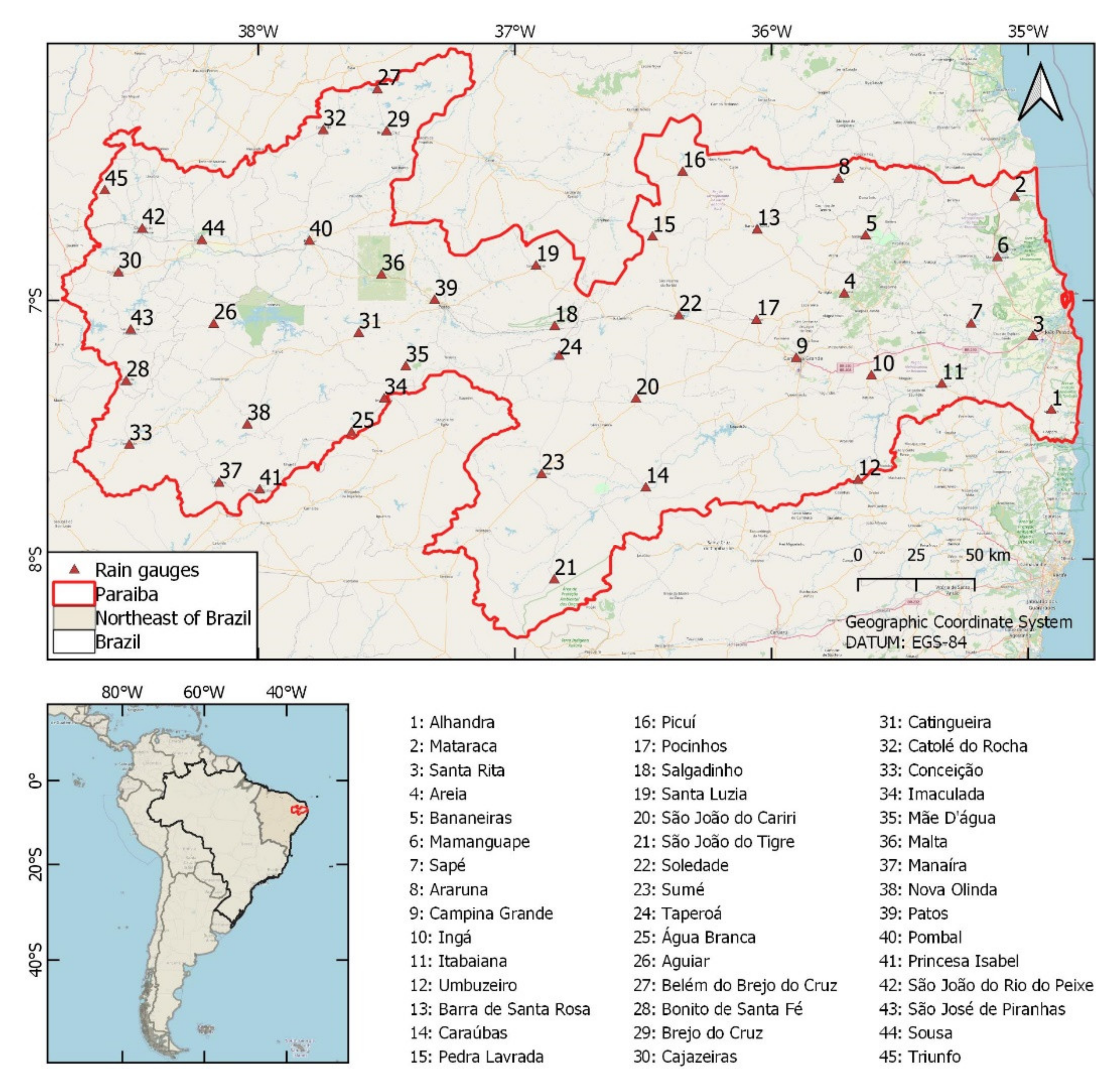
2.1. Study Area
2.2. Data
2.3. Methods
2.3.1. Descriptive Analysis
2.3.2. GAMLSS Model
2.3.3. Model Evaluation Criteria
2.3.4. Efficiency for Seasonal Prediction
3. Results
3.1. Series Investigation
3.2. Application of the GAMLSS Model
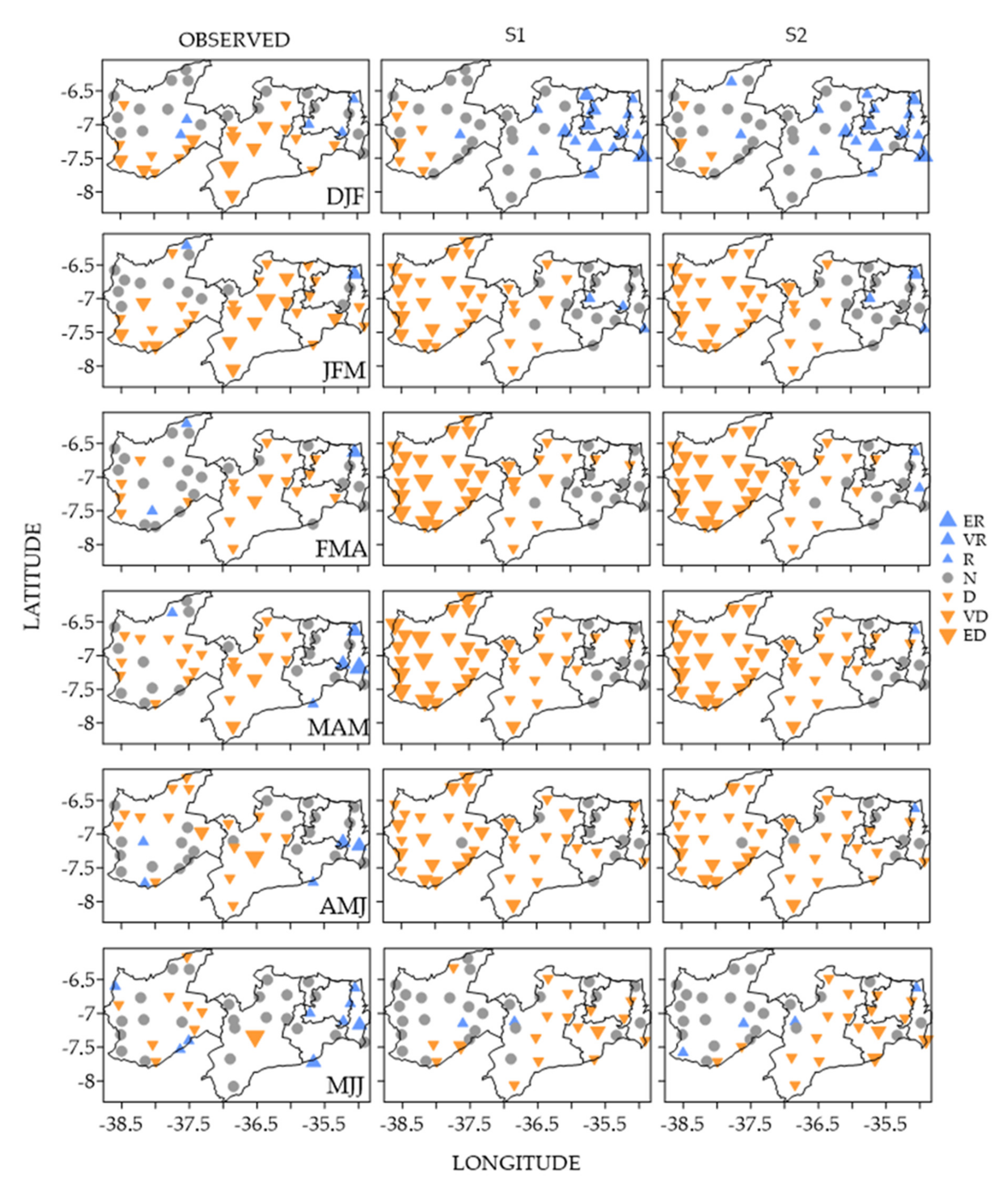
3.3. Quantile Prediction
3.4. Efficiency Indicators
4. Discussion
5. Conclusions
Author Contributions
Funding
Acknowledgments
Conflicts of Interest
References
- Walker, G. World Weather. Word Weather. Mon. Weather Rev. 1928, 56, 167–170. [Google Scholar] [CrossRef]
- Bjerknes, J. Atmospheric teleconnections form the equatorial Pacific. Mon. Weather Rev. 1969, 97, 163–172. [Google Scholar] [CrossRef]
- Andreoli, R.V.; Kayano, M.T. A importância relativa do Atlântico Tropical Sul e Pacífico Leste na variabilidade da precipitação do Nordeste do Brasil. Rev. Bras. Meteorol. 2007, 22, 63–74. [Google Scholar] [CrossRef]
- Nogueira, V.S.; Cavalcanti, E.P.; Nogueira, V.F.B.; Rildo, G.M.; Fernandes, A.A. Oscilação interanual da precipitação observada associada aos sistemas convectivos de mesoescala sobre o estado da Paraíba. Rev. Bras. Geogr. Fís. 2014, 7, 969–978. [Google Scholar]
- Hastenrath, S.; Heller, L.D. Dynamics of climate hazards in northeast Brazil. Q. J. R. Meteorol. Soc. 1977, 103, 77–92. [Google Scholar] [CrossRef]
- Kousky, V.E.; Kayano, M.T.; Cavalcanti, I.F.A. A review of the Southern Oscillation: Oceanic-atmospheric circulation changes and related rainfall anomalies. Tellus A 1984, 36, 490–504. [Google Scholar] [CrossRef] [Green Version]
- Kayano, M.T.; Rao, V.B.; Moura, A.D. Tropical circulation and the associated rainfall anomalies during two contrasting years. J. Clim. 1988, 8, 477–488. [Google Scholar] [CrossRef] [Green Version]
- Kayano, M.T.; Andreoli, R.V. Relationships between rainfall anomalies over northeastern Brazil and the El Niño-Southern Oscillation. J. Geophys. Res. Atmos. 2006, 111. [Google Scholar] [CrossRef] [Green Version]
- Hastenrath, S. Exploring the climate problems of Brazil’s Nordeste: A review. Clim. Chang. 2012, 112, 243–251. [Google Scholar] [CrossRef]
- Hounsou-Gbo, G.A.; Araujo, M.; Bourlès, B.; Veleda, D.; Servain, J. Tropical Atlantic contributions to strong rainfall variability along the Northeast Brazilian coast. Adv. Meteorol. 2015, 1–13. [Google Scholar] [CrossRef] [Green Version]
- Cintra, M.M.; Lentini, C.A.D.; Servain, J.; Araujo, M.; Marone, E. Physical processes that drive the seasonal Evolution of the Southwestern Tropical Atlantic Warm Pool. Dyn. Atmos. Ocean. 2015, 72, 1–11. [Google Scholar] [CrossRef]
- Uvo, C.B.; Repelli, C.A.; Zebiak, S.E.; Kushnir, Y. The relationships between Tropical Pacific and Atlantic SST and Northeast Brazil monthly precipitation. J. Clim. 1998, 11, 551–562. [Google Scholar] [CrossRef]
- Robertson, A.W.; Kirshner, S.; Smyth, P. Downscaling of daily rainfall occurrence over Northeast Brazil using a hidden Markov model. J. Clim. 2004, 17, 4407–4424. [Google Scholar] [CrossRef]
- Andrade, M.M.; Lima, K.C. Projeção climática da frequência de eventos de precipitação intensa no Nordeste do Brasil. Rev. Bras. Geogr. Fís. 2013, 6, 1158–1173. [Google Scholar] [CrossRef] [Green Version]
- Pereira, M.P.S.; Justino, F.; Malhado, A.C.M.; Barbosa, H.; Marengo, J. The influence of oceanic basins on drought and ecosystem dynamics in Northeast Brazil. Environ. Res. Lett. 2014, 9, 1–8. [Google Scholar] [CrossRef] [Green Version]
- Shimizu, M.H.; Ambrizzi, T.; LiebMann, B. Extreme precipitation events and their relationship with ENSO and MJO phases over northern South America. Int. J. Clim. 2016, 37, 2977–2989. [Google Scholar] [CrossRef]
- Marengo, J.A.; Torres, R.R.; Alves, L.M.M. Drought in Northeast Brazil—Past, present, and future. Appl. Clim. 2017, 129, 1189–1200. [Google Scholar] [CrossRef]
- Uvo, C.R.B. A Zona de Convergência Intertropical (ZCIT) e Sua Relação com a Precipitação da Região Norte do Nordeste Brasileiro. Master’s Thesis, National Institute for Space Research (INPE), São Paulo, Brazil, 1989. [Google Scholar]
- Gan, M.A. Um Estudo Observacional Sobre as Baixas Frias da Alta Troposfera, nas Latitudes Subtropicais do Atlântico Sul e Leste do Brasil. Master’s Thesis, National Institute for Space Research (INPE), São Paulo, Brazil, 1982. [Google Scholar]
- Cavalcanti, I.F.A.; Ferreira, N.J.; Dias, M.A.F.; Justi da Silva, M.G.A. Tempo e Clima No Brasil, 1st ed.; Oficina de Textos: São Paulo, Brazil, 2009. [Google Scholar]
- Souza, E.B.; Alves, J.M.B.; Repelli, C.A. Um complexo convectivo de mesoescala associado à precipitação intensa sobre Fortaleza—CE. Rev. Bras. Meteorol. 1998, 13, 1–14. [Google Scholar]
- Ferreira, A.G.; Mello, N.G.S. Principais sistemas atmosféricos atuantes sobre a região Nordeste do Brasil e a influência dos oceanos Pacífico e Atlântico no clima da região. Rev. Bras. Clim. 2005, 1, 15–28. [Google Scholar] [CrossRef] [Green Version]
- Vianello, R.L.; Alves, A.R. Meteorologia Básica e Aplicações, 2nd ed.; Federal University of Viçosa (UFV): Minas Gerais, Brazil, 2012. [Google Scholar]
- Moura, A.D.; Shukla, J. On the dynamics of droughts in northeast Brazil: Observations, theory and numerical experiments with a general circulation model. J. Atmos. Sci. 1981, 38, 2653–2675. [Google Scholar] [CrossRef] [Green Version]
- Marengo, J.A.; Alves, L.M.; Beserra, E.A.; Lacerda, F.F. Variabilidade e mudanças climáticas no semiárido brasileiro. Recursos Hídricos em Regiões Áridas e Semiáridas; Instituto Nacional do Semiárido: Paraíba, Brazil, 2011. [Google Scholar]
- Sampaio, F.J. Iminência duma grande seca nordestina. Revista Brasileira Geografia 1950, 12, 3–15. [Google Scholar]
- Marinho, M.E.; Rebouças, A.C. Hidrologia das Secas: Nordeste do Brasil; Sudene: Pernambuco, Brazil, 1970. [Google Scholar]
- CNM—National Confederation of Municipalities (Portuguese, Confederação Nacional de Municípios). Decretações de Anormalidades Causadas por Desastres nos Municípios Brasileiros. Desenvolvimento Territorial—Proteção e Defesa Civil—Brasília: CNM. 2018. Available online: https://www.cnm.org.br/cms/biblioteca/documentos/Decretacoes-de-anormalidades-causadas-por-desastres-nos-Municipios-Brasileiros-10-10-2018-v2.pdf (accessed on 17 July 2019).
- Morettin, P.A.; Toloi, C. Análise de Séries Temporais, 2nd ed.; Blucher: São Paulo, Brazil, 2006. [Google Scholar]
- Bayer, D.M.; Castro, N.M.R. Modelagem e Previsão de Vazões Médias Mensais do Rio Potiribu Utilizando Modelos de Séries Temporais. RBRH 2012, 17, 229–239. [Google Scholar] [CrossRef]
- Fathian, F.; Mehdizadeh, S.; Sales, A.K.; Safari, M.J.S. Hybrid models to improve the monthly river flow prediction: Integrating artificial intelligence and non-linear time series models. J. Hydrol. 2019, 575, 1200–1213. [Google Scholar] [CrossRef]
- Mehdizadeh, S.; Fathian, F.; Adamowski, J.D. Hybrid artificial intelligence-time series models for monthly streamflow modeling. Appl. Soft Comput. 2019, 80, 873–887. [Google Scholar] [CrossRef]
- Rigby, R.A.; Stasinopoulos, D.M. Generalized additive models for location, scale and shape. J. R. Stat. Soc. C Appl. 2005, 54, 507–554. [Google Scholar] [CrossRef] [Green Version]
- Gao, L.; Huang, J.; Chen, X.; Chen, Y.; Liu, M. Contributions of natural climate changes and human activities to the trend of extreme precipitation. Atmos. Res. 2018, 205, 60–69. [Google Scholar] [CrossRef]
- Medeiros, E.S.; Lima, R.R.; Olinda, R.A.; Dantas, L.G.; Santos, C.A.C. Space-time krigin of precipitation: Modeling the large-scale variation with model GAMLSS. Water 2019, 11, 2368. [Google Scholar] [CrossRef] [Green Version]
- Rashid, M.M.; Beecham, S. Simulation of stream with statistically downscaled daily rainfall using a hybrid of wavelet and GAMLSS models. Hydrol. Sci. J. 2019, 64, 1327–1339. [Google Scholar] [CrossRef]
- Rydén, J. A note on analysis of extreme minimum temperatures with the GAMLSS framework. Acta Geophys. 2019, 67, 1599–1604. [Google Scholar] [CrossRef] [Green Version]
- Das, J.; Jha, S.; Goyal, M.K. Non-stationary and copula-based approach to assess the drought characteristics encompassing climate indices over the Himalayan sates in India. J. Hydrol. 2020, 580. [Google Scholar] [CrossRef]
- Tan, X.; Gan, T.Y. Non-stationary analysis of annual maximum streamflow of Canada. J. Clim. 2015, 28, 1788–1805. [Google Scholar] [CrossRef]
- Stasinopoulos, D.M.; Rigby, R.A. Generalized Additive Models for Location Scale and Shape (GAMLSS) in R. J. Stat. Softw. 2007, 23, 1–46. [Google Scholar] [CrossRef] [Green Version]
- Villarini, G.; Smith, J.A.; Serinaldi, F.; Bales, J.; Bates, P.D.; Krajewski, W.F. Flood frequency analysis for non-stationary annual peak records in an urban drainage basin. Adv. Water Resour. 2009, 32, 1255–1266. [Google Scholar] [CrossRef]
- Van Ogtrop, F.F.; Vervoort, R.W.; Heller, G.Z.; Stasinopoulos, D.M.; Rigby, R.A. Long-range forecasting of intermittent streamflow. Hydrol. Earth Syst. Sc. 2011, 15, 3343–3354. [Google Scholar] [CrossRef] [Green Version]
- Voudoris, V.; Gilchrist, R.; Rigby, R.; Sedgwick, J.; Stasinopoulos, D. Modelling skewness and kurtosis with the BCPE density in GAMLSS. J. Appl. Stat. 2012, 36, 1279–1293. [Google Scholar] [CrossRef]
- López, J.; Francés, F. Non-stationary flood frequency analysis in continental Spanish rivers, using climate and reservoir indices as external covariates. Hydrol. Earth Syst. Sci. 2013, 17, 3189–3203. [Google Scholar] [CrossRef] [Green Version]
- Gu, X.; Zhang, Q.; Li, J.; Singh, V.P.; Sun, P. Impact of urbanization on nonstationarity of annual and seasonal precipitation extremes in China. J. Hydrol. 2019, 575, 638–675. [Google Scholar] [CrossRef]
- Apurv, T.; Cai, X. Evaluation of the stationary assumption for meteorological drought risk estimation at the multidecadal scale in contiguous United States. Water Resour. Res. 2019, 55, 5074–5101. [Google Scholar] [CrossRef]
- IBGE—Brazilian Institute of Geography and Statistics (Portuguese, Instituto Brasileiro de Geografia e Estatística. 2017. Available online: https://cidades.ibge.gov.br/brasil/pb/panorama (accessed on 1 January 2018).
- ANA—National Water Agency of Brazil (Portuguese, Agência Nacional de Águas. 2018. Available online: http://www.snirh.gov.br/hidroweb/publico/medicoes_historicas_abas.jsf (accessed on 2 February 2018).
- AESA—State Water Resources Management Executive Agency (Portuguese, Agência Executiva de Gestão das Águas do Estado da Paraíba. 2018. Available online: http://www.aesa.pb.gov.br/aesa-website/meteorologia-chuvas/ (accessed on 2 February 2018).
- CPC/NCEP/NOAA—Climate Prediction Center/National Centers for Evironmental Prediction/National Oceanic and Atmospheric Administration. 2018. Available online: http://www.cpc.ncep.noaa.gov/data/indices/ (accessed on 2 February 2018).
- ESRL/NOAA—Earth System Research Laboratory/National Oceanic & Atmospheric Administration. 2018. Available online: https://www.esrl.noaa.gov/psd/data/climateindices/list/ (accessed on 2 February 2018).
- R Development Core Team. R: A Language and Environment for Statistical Computing. R Foundation for Statistical Computing, Vienna, Austria. 2019. Available online: http://cran.r-project.org/index.html (accessed on 13 December 2019).
- Dantas, L.G.; Santos, C.A.C.; Olinda, R.A. Tendências anuais e sazonais nos extremos de temperatura do ar e precipitação em Campina Grande—PB. Rev. Bras. Meteorol. 2015, 30, 423–434. [Google Scholar] [CrossRef] [Green Version]
- Honaker, J.; King, G.; Blackwell, M. Amelia II: A program for missing data. J. Stat. Softw. 2011, 45, 1–47. [Google Scholar] [CrossRef]
- Dantas, L.G.; Santos, C.A.C.; Olinda, R.A. Reamostragem de séries pluviométricas no estado da Paraíba. Rev. Bras. Geogr. Fís. 2016, 9, 997–1006. [Google Scholar] [CrossRef] [Green Version]
- Gilabert, M.B.; Cobelas, M.A.; Angeler, D.G. Effects of climatic change on stream water quality in Spain. Clim. Chang. 2010, 103, 339–352. [Google Scholar] [CrossRef]
- Sheng, H.; Liu, H.; Wang, C.; Guo, H.; Liu, Y.; Yang, Y. Analysis of cyanobacteria bloom in the Waihai part of Dianchi Lake, China. Ecol. Inf. 2012, 10, 37–48. [Google Scholar] [CrossRef]
- Kruyt, B.; Lehning, M.; Kahl, A. Potential contributions of wind power to a stable and highly renewable Swiss power supply. Appl. Energy 2017, 192, 1–11. [Google Scholar] [CrossRef] [Green Version]
- Revelle, W. Hierarchical cluster analysis and the internal structure of tests. Multivar. Behav. Res. 1979, 14, 57–74. [Google Scholar] [CrossRef]
- Milligan, G.W.; Cooper, M.C. A study of the comparability of external criteria for hierarchical cluster analysis. Multivar. Behav. Res. 1986, 21, 441–458. [Google Scholar] [CrossRef]
- Santos, C.A.G.; Neto, R.M.B.; Silva, R.M.; Costa, S.G.F. Cluster analysis apllied to spatiotemporal variability of monthly precipitation over Paraíba state using Tropical Rainfall Measuring Mission (TRMM) data. Remote Sens. 2019, 11, 637. [Google Scholar] [CrossRef] [Green Version]
- Oliveira, P.T.; Santos e Silva, C.M.S.; Lima, K.C. Climatology and trend analysis of extreme precipitation in subregions of Northeast Brazil. Appl. Clim. 2017, 130, 77–90. [Google Scholar] [CrossRef]
- Kassambara, A.; Mundt, F. Factoextra: Extract and Visualize the Results of Multivariate Data Analyses. R Package Version 1.0.5. 2017. Available online: https://CRAN.R-project.org/package=factoextra (accessed on 13 December 2019).
- Murtagh, F.; Legendre, P. Ward’s hierarchical agglomerative clustering method: Which algorithms implement ward’s criterion? J. Classif. 2014, 31, 274–295. [Google Scholar] [CrossRef] [Green Version]
- Von Storch, V.H. Misuses of statistical analysis in climate research. In Analysis of Climate Variability: Applications of Statistical Techniques; von Storch, H., Navarra, A., Eds.; Springer: Berlin, Germany, 1995; pp. 11–26. [Google Scholar] [CrossRef]
- Yue, S.; Wang, C.Y. Applicability of prewhitening to eliminate the influence of serial correlation on the Mann-Kendall test. Water Resour. Res. 2012, 38, 1–7. [Google Scholar] [CrossRef]
- Blain, G.C. The Mann-Kendall test: The need to consider the interaction between serial correlation and trend. Acta Sci. Agron. 2013, 35, 393–402. [Google Scholar] [CrossRef]
- Verma, M.K.; Swain, S. Statistical analysis of precipitation over seonath River Basin, Chhattisgarh, India. Int. J. App. Eng. Res. 2016, 11, 2417–2423. [Google Scholar] [CrossRef]
- Gu, X.; Zhang, Q.; Singh, V.P.; Liu, L.; Shi, P. Spatiotemporal patterns of annual and seasonal precipitation extreme distributions across China and potential impact of tropical cyclones. Int. J. Clim. 2017, 37, 3949–3962. [Google Scholar] [CrossRef]
- Chan, K.S.; Ripley, B. TSA: Time Series Analysis. R Package Version. 2012. Available online: https://CRAN.R-project.org/package=TSA (accessed on 13 December 2019).
- Villarini, G.; Smith, J.A.; Napolitano, F. Non-stationary modeling of a long record of rainfall and temperature over Rome. Adv. Water Resour. 2010, 33, 1256–1267. [Google Scholar] [CrossRef]
- Villarini, G.; Serinaldi, F. Development of statistical models for at-site probabilistic seasonal rainfall forecast. Int. J. Clim. 2012, 32, 2197–2212. [Google Scholar] [CrossRef]
- Zhang, D.D.; Yan, D.H.; Wang, Y.C.; Lu, F.; Liu, S.H. GAMLSS-based non-stationary modeling of extreme precipitation in Beijing-Tianjin-Hebei region of China. Nat. Hazards 2015, 77, 1037–1053. [Google Scholar] [CrossRef]
- Cribari-Neto, F.; Lucena, S.E.F. Non-nested hypothesis testing inference for GAMLSS modes. J. Stat. Comput. Sim. 2016, 87, 1189–1205. [Google Scholar] [CrossRef]
- Gao, L.; Huang, J.; Chen, X.; Chen, Y.; Liu, M. Risk of extreme precipitation under non-stationary conditions during the second flood season in the southeastern coastal region of China. J. Hydrometeorol. 2017, 18, 669–681. [Google Scholar] [CrossRef]
- Rashid, M.M.; Beechman, S. Development of a non-stationary Standardized Precipitation Index and its application to a South Australian climate. Sci. Total Environ. 2019, 657, 882–892. [Google Scholar] [CrossRef]
- Stasinopoulos, M.D.; Rigby, R.A.; Heller, G.Z.; Voudouris, V.; De Bastiani, F. (Eds.) Flexible Regression and Smoothing: Using GAMLSS in R; Chapman and Hall/CRC The R Series: Boca Raton, FL, USA, 2017. [Google Scholar] [CrossRef]
- Akaike, H. A new look at the statistical model identification. IEEE Trans. Autom. Control 1974, 19, 716–723. [Google Scholar] [CrossRef]
- Schwarz, G. Estimating the dimension of a model. Ann. Stat. 1978, 6, 461–464. [Google Scholar] [CrossRef]
- Filliben, J.J. The probability plot correlation coeficient test for normality. Technometrics 1975, 17, 111–117. [Google Scholar] [CrossRef]
- Van Buuren, S.; Fredriks, M. Worm plot: A simple diagnostic device for modelling growth reference curves. Stat. Med. 2001, 20, 1259–1277. [Google Scholar] [CrossRef] [PubMed]
- Tyralis, H.; Papacharalampous, G.; Tantanee, S. How to explain and predict the shape parameter of the generalized extreme value distribution of streamflow extremes using a big dataset. J. Hydrol. 2019, 574, 628–645. [Google Scholar] [CrossRef]
- Khouakhi, A.; Villarini, G.; Zhang, W.; Slater, L.J. Seasonal predictability of high sea level frequency using ENSO patterns along the U.S. West Coast. Adv. Water Resour. 2019, 131. [Google Scholar] [CrossRef]
- Pinkayan, S. Conditional Probabilities of Occurrence of Wet and Dry Years over a Large Continental Area. Hydrology Papers, n. 12; Colorado State University: Fort Collins, CO, USA, 1966. [Google Scholar]
- Xavier, T.M.B.S. A Técnica Dos Quantis e Suas Aplicações em Meteorologia, Climatologia e Hidrologia, Com Ênfase Para as Regiões Brasileiras; Thesaurus: Brasília, DF, Brazil, 2002. [Google Scholar]
- Kayano, M.T.; Capistrano, V.B.; Andreoli, R.V.; Souza, R.A.F. A further of the tropical Atlantic SST modes and their relations to north-eastern Brazil rainfall during different phases of Atlantic Multidecadal Oscillation. Int. J. Clim. 2016, 36, 4006–4018. [Google Scholar] [CrossRef] [Green Version]
- Tavares, A.L.; Carmo, A.M.C.; Silva Júnior, R.O.; Souza-Filho, P.W.M.; Silva, M.S.; Ferreira, D.B.S.; Nascimento Júnior, W.R.; Dall’agnol, R. Climate indicators for a watershed in the eastern amazon. Rev. Bras. Clim. 2018, 23, 389–410. [Google Scholar] [CrossRef]
- Hyndman, R.J.; Fan, Y. Sample quantiles in statistical packages. Am. Stat. 1996, 50, 361–365. [Google Scholar] [CrossRef]
- Capozzoli, C.R.; Cardoso, A.O.; Ferraz, S.E.R. Padrões de variabilidade de vazão de rios nas principais bacias brasileiras e associação com índices climáticos. Rev. Bras. Meteorol. 2017, 32, 243–254. [Google Scholar] [CrossRef] [Green Version]
- Alves, J.M.B.; Repelli, C.A. A variabilidade pluviométrica no setor norte do Nordeste e os eventos El Niño-Oscilação Sul (ENOS). Rev. Bras. Meteorol. 1992, 7, 583–592. [Google Scholar]
- Alves, J.M.B.; Souza, R.O.; Campos, J.N.B. Previsão da anomalia de temperatura da superfície do mar (TSM) no atlântico tropical, com a equação da difusão de temperatura. Rev. Climaná. 2003, 1, 6–19. [Google Scholar]
- Moura, G.B.A.; Aragão, J.O.R.; Melo, J.S.P.; Silva, A.P.N.; Giongo, P.R.; Lacerda, F.F. Relação entre a precipitação do leste do Nordeste do Brasil e a temperatura dos oceanos. Rev. Bras. Eng. Agríc. Ambient. 2009, 13, 462–469. [Google Scholar] [CrossRef] [Green Version]
- Gherardi, D.F.M.; Paes, E.T.; Soares, C.H.; Pezzi, L.P.; Kayano, M.T. Differences between spatial patterns of climate variability and large marine ecosystem in the western South Atlantic. Pan Am. J. Aquat. Sci. 2010, 5, 310–319. [Google Scholar]
- Guerreiro, M.J.S.; Andrade, E.M.; Abreu, I.; Lajinha, T. Long-term variation of precipitation indices in Ceará State Northeast Brazil. Int. J. Clim. 2013, 33, 2929–2939. [Google Scholar] [CrossRef]
- Hounsou-Gbo, G.A.; Servain, J.; Araujo, M.; Caniaux, G.; Bourlès, B.; Fontenele, D.; Martins, E.S.P.R. SST indexes in the Tropical South Atlantic for forecasting rainy seasons in Northeast Brazil. Atmosphere 2019, 10, 335. [Google Scholar] [CrossRef] [Green Version]
- Rashid, M.M.; Beecham, S.; Chowdhury, R.K. Simulation of extreme rainfall and projection of future changes using the GLIMCLIM model. Appl. Clim. 2016, 130, 1–14. [Google Scholar] [CrossRef]
- Rodrigues, J.S. Análise de Diagnóstico em Modelo de Regressão ZAGA e ZAIG. Master’s Thesis, University of São Paulo/Federal University of São Carlos, São Paulo, Brazil, 2016. [Google Scholar]
- Pousa, R.; Costa, M.H.; Pimenta, F.M.; Fontes, V.C.; Brito, V.F.A.; Castro, M. Climate change and intense irrigation growth in western Bahia, Brazil: The urgent need for hydroclimatic monitoring. Water 2019, 11, 933. [Google Scholar] [CrossRef] [Green Version]
- Villarini, G.; Vechhi, G.A.; Smith, J.A. Modeling the dependence of tropical storm counts in the north Atlantic basin on climate indices. Mon. Weather Rev. 2010, 138, 2681–2705. [Google Scholar] [CrossRef]
- Gu, X.; Zhang, Q.; Singh, V.P.; Chen, X.; Liu, L. Nonstationary in the occurrence rate of floods in the Tarim River basin, China, and related impacts of climate indices. Glob. Planet Chang. 2016, 142, 1–13. [Google Scholar] [CrossRef] [Green Version]
- Tong, E.N.C.; Mues, C.; Thomas, L. A zero-adjusted gamma model for mortgage loan loss given default. Int. J. 2013, 29, 548–562. [Google Scholar] [CrossRef] [Green Version]
- Chen, S.; Shao, D.; Tan, X.; Gu, W.; Lei, C. An interval multistage classified model for regional inter- and intra-seasonal water management under uncertain and non-stationary condition. Agric. Water Manag. 2017, 191, 118–128. [Google Scholar] [CrossRef]
- Zhang, Q.; Gu, X.; Singh, V.P.; Xiao, M.; Chen, X. Evaluation of flood frequency under non-stationary resulting from climate indices and reservoir indices in the East River basin, China. J. Hydrol. 2015, 527, 565–575. [Google Scholar] [CrossRef]
- Delgado, J.M.; Voss, S.; Bürguer, G.; Vormoor, K.; Murawski, A.; Pereira, J.M.R.; Martins, E.; Júnior, F.V.; Francke, T. Seasonal drought prediction for semi-arid northeastern Brazil: Verification of six hydro-meteorological forecast products. Hydrol. Earth Syst. Sci. 2018, 22, 5041–5056. [Google Scholar] [CrossRef]
- Martins, E.S.P.R.; Coelho, C.A.S.; Haarsma, R.; Otto, F.E.L.; King, A.D.; Van Oldenborgh, G.J.; Kew, S.; Philip, S.; Júnior, F.C.V.; Cullen, H. A multimethod attribution analysis of the prolonged northeast Brazil hydro-meteorological drought (2012–2016). (in “Explaining Extreme Events of 2016 from a Climate Perspective”). Bull. Am. Meteorol. Soc. 2018, 99, S65–S69. [Google Scholar] [CrossRef]
- Silva, T.L.V.; Veleda, D.; Araujo, M.; Tyaquicã, P. Ocean-atmosphere feedback during extreme rainfall events in eastern Northeast Brazil. J. Appl. Meteorol. Clim. 2018, 57, 1211–1229. [Google Scholar] [CrossRef]
- Tompkins, A.M.; Lowe, R.; Nissan, H.; Martiny, N.; Roucou, P.; Thomson, M.C.; Nakazawa, T. Predicting climate impacts on health at sub-seasonal to seasonal timescales. In The Gap between Weather and Climate Forecasting: Sub-Seasonal to Seasonal Prediction; Vitart, F., Robertson, A., Eds.; Elsevier: Amsterdam, The Netherlands, 2019; pp. 455–477. [Google Scholar] [CrossRef]
- Trenberth, K.E. El Niño Southern Oscillation (ENSO). In Reference Module in Earth Systems and Environmental Sciences, Encyclopedia of Ocean Sciences, 3rd ed.; Elsevier: Amsterdam, The Netherlands, 2017; Volume 6, pp. 420–432. [Google Scholar] [CrossRef]
- Pilz, T.; Delgado, J.M.; Voss, S.; Vormoor, K.; Francke, T.; Costa, A.C.; Martins, E.; Bronsert, A. Seasonal drought prediction for semi-arid northeast Brazil: What is the added value of a process-based hydrological model? Hydrol. Earth Syst. Sci. 2019, 23, 1951–1971. [Google Scholar] [CrossRef] [Green Version]
- Sangelantoni, L.; Ferreti, R.; Redaelli, G. Toward a Regional-Scale Seasonal Climate Prediction System over Central Italy Based on Dynamical Downscaling. Climate 2019, 7, 120. [Google Scholar] [CrossRef] [Green Version]
- Manzanas, R.; Lucero, A.; Weisheimer, A.; Gutiérrez, J.M. Can bias correction and statistical downscaling methods improve the skill of seasonal precipitation forecasts? Clim. Dyn. 2017, 50, 1161–1176. [Google Scholar] [CrossRef] [Green Version]
- Alves, J.M.B.; Silva, E.M.; Sombra, S.S.; Barbosa, A.C.B.; Santos, A.C.S.; Lira, M.A.T. Eventos extremos diários de chuva no Nordeste do Brasil e características atmosféricas. Rev. Bras. Meteorol. 2017, 32, 227–233. [Google Scholar] [CrossRef] [Green Version]
- Nóbrega, J.N. Eventos Extremos de Precipitação nas Mesorregiões do Estado da Paraíba e Suas Relações com a TSM dos Oceanos Atlântico e Pacífico. Master’s Thesis, Federal University of Campina Grande, Paraíba, Brazil, 2012. [Google Scholar]
- Junior, F.C.V.; Jones, C.; Gandu, A.W. Interannual and intraseasonal variations of the onset and demise of the pre-wet season and the wet season in the Northern Northeast Brazil. Rev. Bras. Meteorol. 2018, 33, 472–484. [Google Scholar] [CrossRef] [Green Version]


| Distribution Function | Abbreviation | Probability Density Function |
|---|---|---|
| Gamma | GA | to |
| Generalized Gamma | GG | to |
| Zero Adjusted Gamma | ZAGA | to |
| Gumbel | GU | to |
| Logistic | LO | to |
| Log-Normal | LOGNO | to |
| Weibull | WEI | |
| to |
| Quantiles | Rating |
|---|---|
| p < Q(0.05) | Extremely dry |
| Q(0.05) < p < Q(0.15) | Very dry |
| Q(0.15) < p < Q(0.35) | Dry |
| Q(0.35) < p < Q(0.65) | Normal |
| Q(0.65) < p < Q(0.85) | Rainy |
| Q(0.85) < p < Q(0.95) | Very rainy |
| Q(0.95) < p | Extremely rainy |
| Region | Niño 1 + 2 | Niño 3 | Niño 3.4 | Niño 4 | SOI | AMO | PDO | TNA | TSA |
|---|---|---|---|---|---|---|---|---|---|
| R1 | 0 | 0 | 0 | 7 | 3 | 0 | 0 | 3 | 1 |
| R2 | 0 | 0 | 0 | 7 | 3 | 0 | 0 | 3 | 1 |
| R3 | 0 | 0 | 0 | 7 | 3 | 0 | 0 | 3 | 1 |
| R4 | 2 | 2 | 2 | 6 | 3 | 0 | 0 | 3 | 2 |
| R5 | 2 | 2 | 2 | 6 | 3 | 0 | 0 | 3 | 2 |
| Location | Region | Distribution | AIC | BIC |
|---|---|---|---|---|
| Alhandra | R1 | GG | 4268.73 | 4338.68 |
| Mataraca | R1 | GG | 4042.68 | 4081.54 |
| Santa Rita | R1 | GG | 3978.83 | 4033.24 |
| Areia | R1 | GG | 3954.90 | 4013.20 |
| Bananeiras | R2 | ZAGA | 3946.78 | 3989.53 |
| Mamanguape | R2 | GG | 4000.79 | 4055.20 |
| Sapé | R2 | GG | 3838.31 | 3900.49 |
| Araruna | R3 | GG | 3638.50 | 3696.79 |
| Campina Grande | R3 | GG | 3618.09 | 3656.95 |
| Ingá | R3 | ZAGA | 3571.23 | 3617.87 |
| Itabaiana | R3 | GG | 3571.47 | 3629.76 |
| Umbuzeiro | R3 | ZAGA | 3701.84 | 3752.36 |
| Barra de Santa Rosa | R4 | ZAGA | 3313.38 | 3360.02 |
| Caraúbas | R4 | ZAGA | 3183.71 | 3242.00 |
| Pedra Lavrada | R4 | ZAGA | 3148.88 | 3207.17 |
| Picuí | R4 | ZAGA | 3239.29 | 3285.92 |
| Pocinhos | R4 | ZAGA | 3189.53 | 3240.05 |
| Salgadinho | R4 | ZAGA | 3292.98 | 3335.73 |
| Santa Luzia | R4 | ZAGA | 3344.64 | 3406.82 |
| São João do Cariri | R4 | ZAGA | 3356.13 | 3410.54 |
| São João do Tigre | R4 | ZAGA | 3276.69 | 3334.98 |
| Soledade | R4 | ZAGA | 3297.82 | 3332.80 |
| Sumé | R4 | ZAGA | 3376.54 | 3419.28 |
| Taperoá | R4 | ZAGA | 3501.20 | 3551.72 |
| Água Branca | R5 | ZAGA | 3675.94 | 3730.34 |
| Aguiar | R5 | ZAGA | 3670.64 | 3721.16 |
| Belém do Brejo do Cruz | R5 | ZAGA | 3553.75 | 3592.61 |
| Bonito de Santa Fé | R5 | ZAGA | 3751.72 | 3802.24 |
| Brejo do Cruz | R5 | ZAGA | 3674.20 | 3724.72 |
| Cajazeiras | R5 | ZAGA | 3853.81 | 3896.55 |
| Catingueira | R5 | ZAGA | 3587.68 | 3630.43 |
| Catolé do Rocha | R5 | ZAGA | 3678.56 | 3740.74 |
| Conceição | R5 | ZAGA | 3641.92 | 3711.87 |
| Imaculada | R5 | ZAGA | 3554.64 | 3628.47 |
| Mãe D’Água | R5 | ZAGA | 3463.90 | 3518.31 |
| Malta | R5 | ZAGA | 3612.42 | 3666.82 |
| Manaíra | R5 | ZAGA | 3631.18 | 3689.47 |
| Nova Olinda | R5 | ZAGA | 3714.25 | 3780.31 |
| Patos | R5 | ZAGA | 3656.41 | 3718.59 |
| Pombal | R5 | ZAGA | 3646.57 | 3708.77 |
| Princesa Isabel | R5 | ZAGA | 3694.23 | 3748.63 |
| São João do Rio do Peixe | R5 | ZAGA | 3710.70 | 3776.77 |
| São José de Piranhas | R5 | ZAGA | 3746.43 | 3816.37 |
| Sousa | R5 | ZAGA | 3685.23 | 3739.64 |
| Triunfo | R5 | ZAGA | 3666.80 | 3728.98 |
| Period | Scenario | MAE (mm) | PBIAS (%) | RMSE (mm) | R2 (%) |
|---|---|---|---|---|---|
| DJF | S1 | 59.56 | 55.1 | 60.87 | 0.65 |
| S2 | 71.14 | 65.9 | 75.23 | 0.62 | |
| JFM | S1 | 34.21 | 25.3 | 37.54 | 0.8 |
| S2 | 45.11 | 33.3 | 45.54 | 0.75 | |
| FMA | S1 | 12.95 | −4.2 | 15.02 | 0.96 |
| S2 | 1.31 | 0.5 | 1.64 | 0.99 | |
| MAM | S1 | 85.25 | −34 | 86 | 0.66 |
| S2 | 79.65 | −31.8 | 79.65 | 0.68 | |
| AMJ | S1 | 69.62 | −28.2 | 70.19 | 0.72 |
| S2 | 62.41 | −25.3 | 64.45 | 0.75 | |
| MJJ | S1 | 49.27 | −22 | 69.05 | 0.74 |
| S2 | 48.91 | −18.5 | 64.17 | 0.77 |
| Period | Scenario | MAE (mm) | PBIAS (%) | RMSE (mm) | R2 (%) |
|---|---|---|---|---|---|
| DJF | S1 | 35.31 | 31.5 | 44.53 | 0.81 |
| S2 | 29.19 | 26.2 | 36.89 | 0.84 | |
| JFM | S1 | 25.27 | 17.6 | 30.53 | 0.32 |
| S2 | 19.77 | 12.7 | 23.31 | 0.25 | |
| FMA | S1 | 15.12 | −7.1 | 17.79 | 0.92 |
| S2 | 12.51 | −9.5 | 13.44 | 0.9 | |
| MAM | S1 | 64.68 | −34.6 | 71.69 | 0.64 |
| S2 | 62.57 | −33.5 | 64.78 | 0.66 | |
| AMJ | S1 | 47 | −25.8 | 53.4 | 0.73 |
| S2 | 44.15 | −24.3 | 45.72 | 0.75 | |
| MJJ | S1 | 30.4 | −18.4 | 39.19 | 0.79 |
| S2 | 38.2 | −16.7 | 47.1 | 0.79 |
| Period | Scenario | MAE (mm) | PBIAS (%) | RMSE (mm) | R2 (%) |
|---|---|---|---|---|---|
| DJF | S1 | 44.86 | 15.1 | 45.96 | 0.83 |
| S2 | 37.06 | 1.8 | 37.08 | 0.78 | |
| JFM | S1 | 21.97 | 17.1 | 24.71 | 0.96 |
| S2 | 20.34 | 8.6 | 21.11 | 0.97 | |
| FMA | S1 | 10.49 | 14.8 | 10.59 | 0.87 |
| S2 | 3.58 | 5.1 | 3.62 | 0.95 | |
| MAM | S1 | 15.91 | −16.7 | 17.83 | 0.83 |
| S2 | 22.7 | −23.8 | 23.55 | 0.95 | |
| AMJ | S1 | 12.86 | −12.8 | 13.73 | 0.88 |
| S2 | 21.13 | −21 | 21.3 | 0.79 | |
| MJJ | S1 | 22.67 | −7.6 | 23.79 | 0.86 |
| S2 | 23.02 | −16.5 | 27.82 | 0.78 |
| Period | Scenario | MAE (mm) | PBIAS (%) | RMSE (mm) | R2 (%) |
|---|---|---|---|---|---|
| DJF | S1 | 26.26 | 12.3 | 26.61 | 0.77 |
| S2 | 27.28 | 11.8 | 27.6 | 0.76 | |
| JFM | S1 | 14.86 | −0.2 | 14.86 | 0.88 |
| S2 | 17.6 | −3.7 | 17.69 | 0.83 | |
| FMA | S1 | 8.55 | 15.8 | 10.66 | 0.86 |
| S2 | 5.66 | 10.6 | 7.11 | 0.9 | |
| MAM | S1 | 4.36 | −2 | 4.43 | 0.98 |
| S2 | 3.09 | −3.2 | 3.31 | 0.97 | |
| AMJ | S1 | 10.03 | 26.8 | 12.35 | 0.86 |
| S2 | 9.44 | 25.9 | 11.74 | 0.86 | |
| MJJ | S1 | 13.13 | 68.5 | 16.68 | 0.76 |
| S2 | 13.11 | 68.4 | 17.11 | 0.77 |
| Period | Scenario | MAE (mm) | PBIAS (%) | RMSE (mm) | R2 (%) |
|---|---|---|---|---|---|
| DJF | S1 | 15.33 | −16.8 | 20.28 | 0.82 |
| S2 | 20.58 | −17.1 | 24.64 | 0.81 | |
| JFM | S1 | 52.9 | −40.3 | 54.47 | 0.59 |
| S2 | 55.35 | −42.3 | 59.26 | 0.56 | |
| FMA | S1 | 47.08 | −37.6 | 52.52 | 0.61 |
| S2 | 49.75 | −39.8 | 52.34 | 0.59 | |
| MAM | S1 | 44.77 | −42.3 | 46.1 | 0.57 |
| S2 | 43.65 | −41.2 | 44.29 | 0.59 | |
| AMJ | S1 | 24.41 | −9.2 | 24.94 | 0.79 |
| S2 | 22.77 | −3.8 | 22.87 | 0.84 | |
| MJJ | S1 | 16.64 | 48.5 | 21.79 | 0.89 |
| S2 | 18.84 | 64.9 | 24.98 | 0.8 |
© 2020 by the authors. Licensee MDPI, Basel, Switzerland. This article is an open access article distributed under the terms and conditions of the Creative Commons Attribution (CC BY) license (http://creativecommons.org/licenses/by/4.0/).
Share and Cite
Dantas, L.G.; Santos, C.A.C.d.; Olinda, R.A.d.; Brito, J.I.B.d.; Santos, C.A.G.; Martins, E.S.P.R.; de Oliveira, G.; Brunsell, N.A. Rainfall Prediction in the State of Paraíba, Northeastern Brazil Using Generalized Additive Models. Water 2020, 12, 2478. https://doi.org/10.3390/w12092478
Dantas LG, Santos CACd, Olinda RAd, Brito JIBd, Santos CAG, Martins ESPR, de Oliveira G, Brunsell NA. Rainfall Prediction in the State of Paraíba, Northeastern Brazil Using Generalized Additive Models. Water. 2020; 12(9):2478. https://doi.org/10.3390/w12092478
Chicago/Turabian StyleDantas, Leydson G., Carlos A. C. dos Santos, Ricardo A. de Olinda, José I. B. de Brito, Celso A. G. Santos, Eduardo S. P. R. Martins, Gabriel de Oliveira, and Nathaniel A. Brunsell. 2020. "Rainfall Prediction in the State of Paraíba, Northeastern Brazil Using Generalized Additive Models" Water 12, no. 9: 2478. https://doi.org/10.3390/w12092478