The results from the previous section are used to build a predictive model. Firstly, an RF is built, tuned and tested using easily observable features available at the time where the output (FoS) is required, i.e., a real-time assessment (RF and RF). This analysis is then extended utilising crack area as an important feature, which is not, at this present time, considered observable (RF). Secondly, an RF is built, tuned and tested using easily observable features available 15 days prior to when the FoS is required, i.e., a short-term assessment (RF). This analysis is then extended in two ways, using the same additional feature (RF) and reducing the time period of the short-term prediction to 5 days (RF).
3.3.2. Real-Time Assessment
The RF
model is built and trained based on the selected hyper-parameters and features. The feature importance values constitute the relative predictive power of the features and are shown in
Table 4, where surface displacement (
) is seen to have the highest importance, 0.42. It is also shown in
Section 3.2 that
has a strong correlation with FoS. Cumulative rainfall during the last 65 days (
) has the second highest importance, with a feature importance of 0.22, and
at the event day has a lower importance of 0.17. The feature importance of both vegetation growth over the past 15 days (
) and temperature (
) are low, 0.1 and 0.07 respectively. The displacement is the most direct proxy for the water effect within the dike, whereas the rainfall amount and amount of vegetation and temperature influence the water flux, therefore it is logical that they have a lower importance. The rate of vegetation growth is influenced by various climatic variables, and was seen previously [
41] to have a different response at different times of the year, therefore it is reasonable for it to have the lowest importance.
Figure 10a,b show the predicted FoS versus the numerically calculated FoS for the test set and the evaluation set, respectively. The points in these two plots are colourised based on
. The coefficient of correlation (R) between the predicted and calculated FoS in the test data set is 0.94 and RMSE = 0.05. It is clear that the model performs well on the unseen data (test set) that is within its training sample space (
Figure 10a). However, when it comes to the evaluation set, the model performance deteriorates (
Figure 10b); R = 0.31 and RMSE = 0.1. The latter value is considered a high error, since the range of calculated FoS in 2018 is from (almost) 0.8 to 1.4 (although both the R and RMSE are affected by the lower range of values). The variation of predicted and calculated FoS in 2018 is shown by the left-hand side y-axis and the dashed and dotted lines, and precipitation in the same period is shown by the right-hand side y-axis and starts in
Figure 10c. The low performance of the RF
on the evaluation set can be explained based on the latter figure; until further crack growth takes place, the predicted FoS is very close to the calculated FoS (before 22 July 2018) (R = 0.82; RMSE = 0.04). This is also reflected on
Figure 10b by orange markers close to the diagonal line. Once cracks start growing after 22 July 2018, the predicted FoS deviates from the calculated FoS (red markers on
Figure 10b). This is particularly clear on the day with the heaviest precipitation in September 2018 (see
Figure 10c), which causes a large drop in calculated FoS. The (red) markers with the highest distance from the diagonal line correspond to rainy days after crack growth in July 2018. The RF
cannot capture the response to the heavy rainfall which occurs in this period.
As explained in
Section 3.1, when cracks grow, the calculated FoS is affected by
and precipitation events (drop in FoS in August 2018). This shows that the model could not generalise (extrapolate) well on the training data before 2018. This is mainly attributed to the combination of rainfall intensity and unprecedented crack area. In order to investigate the effect of rainfall intensity on the same day that FoS is calculated, this parameter also included as a feature in building the next predictive model, RF
. The feature importance of this model is similar to RF
(
Table 4), except that the added feature (
) has a very low impact on generally predicting FoS. Since the general results of these two models are almost the same, only the time series plot is shown in
Figure 10d. The R value between the predicted and calculated FoS in the test data set is 0.96 and RMSE = 0.05 for RF
, and in the evaluation data set, R = 0.32 and RMSE = 0.10. Using
, the performance of the predictive models improves on days with heavy rainfall, e.g., in April and October 2018, where example results are emphasised with the blue box around them. In these periods, the predicted FoS using RF
is responsive to significant rainfall events, where the predicted FoS drops, following the trends in the calculated results, which is significant for predicting unsafe situations.
In an attempt to improve RF performance, a new model (RF
) is built using
as a feature, along with other features. The feature importance is shown in
Table 4.
has the highest importance among the other features (0.47).
has the second highest feature importance (0.25) and then it is followed by other features. The importance order of the observable features follows RF
.
In
Figure 11a,b, the predicted FoS from the testing and evaluation data set using the RF
model is plotted against the calculated FoS in the corresponding data set, respectively. The R value between the predicted and calculated FoS in the test data set increased to 0.98 and the RMSE decreased to 0.03 (in respect to R = 0.96 and RMSE = 0.05 for RF
). For the evaluation data set, R = 0.56 and the RMSE = 0.07, an improvement compared to the RF
model performance over the evaluation data set (year 2018). According to the time series plot (
Figure 11c), the overall performance of RF
is improved compared to RF
. Yet, the predicted values over-estimate the FoS after the crack expands on 22 July 2018, mostly due to the unprecedented low values, as explained before. In addition, the RF
model has a significantly smaller response to the heavy rainfall events in August–September 2018 than observed. According to
Table 4,
has relatively low influence (feature importance = 0.11) on the FoS prediction. This causes a deviation in the predicted FoS for results after crack growth from the calculated FoS (red points in
Figure 11c). However, when there is no heavy rainfall, e.g., in October 2018, RF
performs well.
In total, when including the crack area as an input feature, in addition to those in the previous model, the model performance improves. It remains a difficult to observe feature, but warrants further investigation given its importance.
Results of this section show that the built RF models have low accuracy after the new trend takes place after growing cracks in summer 2018, because the RF model is not trained for the maximum crack area period. If an RF algorithm was trained over more diverse data of different cases, the RF models may have better performance.
3.3.3. Short Term Prediction
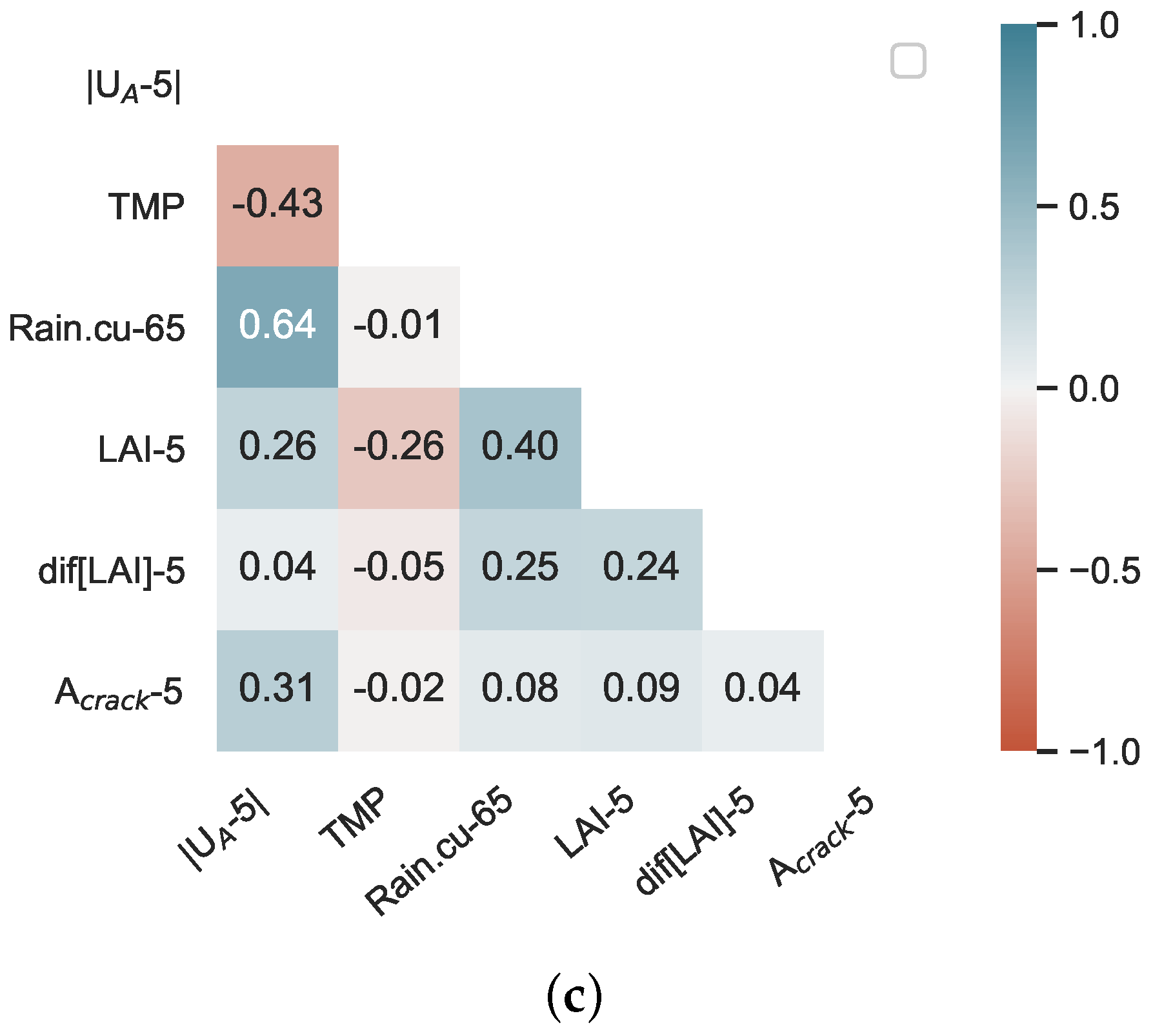
In this section, it is investigated whether an RF algorithm can give a short-term forecast for the dike safety. The used features are the same as before but for an earlier time.
,
and
are selected 15 days before the event day. It is known that these have a lower correlation (see
Figure 7), however this gives sufficient time to undertake further inspection and take action. To enhance RF performance, the meteorological data are used based on the event day, assuming that the climate data are predicted from different climate models which are quite reliable. The time of 15 days is selected as a period, where both the meteorological predictions may be reasonably accurate and which gives the dike managers enough time to take emergency inspection and remedial actions.
In
Table 5, the feature importance for short-term prediction (15d) is shown. Like the previous analysis of RF
,
, 15 days before the event day (i.e.,
), it has the maximum effect on FoS prediction, with the feature importance of 0.32. This is because, even with a 15-day lag, the correlation between displacement and FoS is relatively strong, −0.44 (
Figure 7f).
places in the second rank with the feature importance of 0.23, which does not have the 15 days lag, and the data up to the event day are used, considering the earlier assumption of meteorological data for the next 15 days.
has the feature importance of 0.22. The feature importance of
and
have the least impact on the FoS prediction, like the previous analysis in
Section 3.3.2, since these two features have a very low correlation with FoS (
Figure 7e,f).
The results in
Figure 12a, which are coloured by
, show that for RF
, R = 0.94 and RMSE = 0.06. The results for the evaluation data set (
Figure 12b) show poor performance, i.e., R = 0.06 and RMSE = 0.14. As discussed before for RF
, in the evaluation data set, after cracks grow, the red markers diverge from the diagonal line, showing the deviation of predicted FoS from calculated FoS after 22 July 2018. The markers that have the highest error in prediction correspond to heavy rainfall after crack expansion and cause reductions in calculated FoS, while RF
cannot predict these values. In
Figure 12b,c, the predicted FoS over 2018 is plotted against the calculated FoS in the independent data set. As before, it is seen that after the crack growth, the RF
model cannot predict FoS accurately.
In an attempt to improve the results, two other analyses are tested. Firstly, as in the real-time assessment, the crack area is also considered as one of the features (RF); secondly, the period of the short term prediction decreased to 5 days (RF). For the former option, is selected from 15 days before the event day, and the other features remain as in the RF model.
As expected from previous analyses, has the highest impact on the RF performance (0.48); this is followed by with a feature importance of 0.17. Again, the order of the feature importance for the rest of the features is the same as in the previous analysis. has the relative importance of 0.13, then followed by with the relative importance of 0.11. The lowest relative importance is again for and .
The results of RF
are shown in
Figure 13. The performance of the RF
model is increased compared to RF
over both testing and evaluation data sets. Adding
leads to a higher correlation between predicted and calculated FoS in the testing data set; R increased in order of 0.04 (R = 0.98) and RMSE is reduced by 0.02 (RMSE = 0.04) for the evaluation data set. Again, it can be inferred that after additional crack growth, the model cannot extrapolate FoS values for the heavy rainfall events, since the relative power of antecedent rainfall in predicting FoS is relatively low (feature importance
= 0.13).
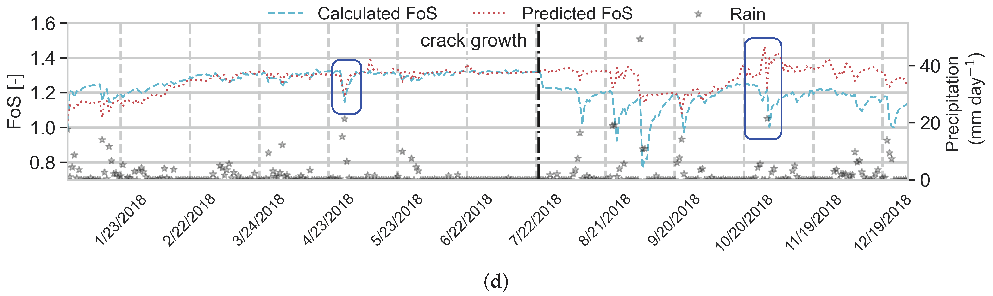
In another attempt to improve the short term prediction models, the lag is reduced to 5 days, which means that , and are selected from 5 days before the event day, while and are selected from the same day that FoS is predicted; is no longer considered. This period can be considered as sufficient to take emergency actions before a dike fails, e.g., evacuating a residential area.
The feature importance of RF
model is shown in
Table 5. Like the previous models,
has the highest importance among other features, 0.36; this is between feature importance for
in real-time assessment and
for short-term prediction (15 days). The reason can be also concluded from
Figure 7b: as the time lag increases, the correlation between FoS and
decreases. The ranking order for other features for the RF
is the same as short-term prediction with 15 days lag. However, the correlation between predicted and calculated FoS is increased in RF
, R= 0.24 and RMSE= 0.12, compared to RF
. As the lag decreases, the correlation between FoS and
and
increases, which leads to an increase in the power of the features in predicting the FoS. The time series plot for 5 days’ prediction is shown in
Figure 14c (again like the previous analysis), the predicted FoS after crack growth in July 2018, which deviates from the calculated FoS. Although in RF
, the deviation is less from the actual FoS compared to the results of RF
, it still performed poorer than RF
.
A summary of the build RF regressor ability to predict the FoS is given in
Table 6, for the training data set, testing data set (which are randomly selected over the years 2009–2017) and the evaluation data set (year 2018). In both scenarios (real-time assessment and short-term prediction), if the crack area is used as one of the features, the model performance improves both in the testing data set and in the evaluation data set. In short-term prediction, when the time window is shortened from 15 days to 5 days, the RF model performance improves, since there is a higher correlation between the features that have the highest impact (
,
and
) and FoS at the shorter lag. Currently, it is not feasible to measure the crack area, but there are ongoing studies to simulate the crack volume, e.g., [
57].
As shown in the results, using a RF regressor, the predicted values are never outside the training set values for the target variable (FoS). One of the RF regressor limitations is that it cannot extrapolate, because in the test set, it predicts an average of the values seen previously in the training. Therefore, the predicted FoS is bound to the minimum and maximum values of the build RF models seen in the training set. In the evaluation data set RF cannot, therefore, predict the minimum FoS values of the whole timeseries (2009–2018) that occurred after the training data set where the maximum
occurs. To overcome this limitation, other algorithms can be used, e.g., deep learning, or combining predictors using stacking [
47]. An alternative could be to undertake more numerical simulations of potential future scenarios to allow the RF regressor to ‘see’ potential future results. This research introduces that using a combination of EO data and predictive models can have a significant potential in the context of dike monitoring. This helps dike managers to be able to undertake real-time assessment and short-term predictions.


