Abstract
Roller compacted concrete (RCC) dams own a large number of horizontal construction layers, which can easily lead to weak joints among layers and generate interlayer joints with different scales to reduce the dam bearing capacity. In this study, extended finite element method (XFEM) is used to simulate crack propagation, the finite element description is first taken on the strong discontinuity. Subsequently, the displacement function of the crack-tip in the quadrilateral element and the geometric determination method of the crack-tip strengthening region are established. Afterwards, the discrete form of the governing equation is derived and the XFEM increment discretization method of the cohesive crack with the crack-tip reinforcement is proposed using the virtual node method to represent the discontinuity of the fracture element. These methods are validated through simulating mixed-mode cracking of one-sided notched asymmetric four-point bending beam. Eventually, the proposed methods are applied to RCC gravity dam to study the development rule and propagation path of the interlayer joints, so as to evaluate the effect of different lengths of the interlayer joints on the dam structural performance. The estimated critical values of dam deformation are helpful to prevent the dam failure during long term operation.
1. Introduction
Roller compacted concrete (RCC) dams are usually built in thin and horizontal lifts, which allow rapid construction and gain recognition for building new dams and rehabilitating existed dams. Roller compacted layer thickness is usually only a few tens of centimeters, resulting in a large number of horizontal construction layers. Over the past four decades, a number of design technologies and construction methods have been adopted to enhance the final product while maintaining the construction speed. However, the weak bonding surfaces among compacted layers still easily crack with different scales, due to material properties, concrete mixed ratio, construction technology, climate conditions and other uncertain factors. For example, 5 of the 10 horizontal cracks on the RCC dam surface of the Fenhe reservoir two were located at the interlaminar junction (including a transmissible horizontal crack with 170 m length appeared at the 874 m elevation of the shutdown surface in the winter of 1998) [1]. Cracks in horizontal construction joints near the dam crest of the Guanyingge occurred when concrete pouring stopped in the upper and lower reaches from late October to early April of the following year [2]. The interlayer joints could reduce dam bearing capacity and durability and their further expansion would endanger dam safety operation. It is critical to study the development law of the interlayer joints under environmental loads, so as to evaluate the effect of the interlayer joints on dam structural performance.
Fracture mechanics is primarily used to study the fracture mechanism of the weak surfaces among RCC layers, such as traditional finite element and adaptive mesh [3], joint force release method [4,5], element cohesive force model [6] and embedded discontinuous model [7]. Since an obvious nonlinear softening stage occur after the external stress reaches the admissible strength, the banded fracture zone at the crack tip should be considered. The weighted finite-element method proposed by Rukavishnikov et al. [8] can suppress the singularity caused by the reentrant corner in the crack simulation. In view of the limitations of the finite element method in dealing with cracks with complex shapes, Belytschko [9] and Moës [10] proposed extended finite element method (XFEM) to solve the strong and weak discontinuous problems, such as cracks, voids, inclusions, etc. Tran et al. [11] certified the effectiveness of the elastic crack-tip enrichment in limit load calculation using the XFEM. The XFEM coupled model built by Aghajanzadehet al. [12] was capable of simulating the strain softening phenomenon in predicting the concrete crack development. The linear smoothed XFEM was implemented by Surendran et al. [13] to simulate the crack growth and agreed well with the experimental results.
Due to the RCC properties in each layer, the layered joints tend to fracture on the interfaces during dam construction and operation. The cohesive crack propagation between layered joints has always attracted much attention. The XFEM needs no mesh reconstruction and no preset crack path in simulating crack propagation [10,14]. In order to further improve the calculation accuracy, the stress intensity factors were taken to govern the growth of the cohesive cracks by Moës et al. [15] and Wolff et al. [16]. Yan et al. [17] derived more suitable crack-tip enrichment functions using the Newmark method. Remmers et al. [18] proposed cohesive segments to represent the crack and insert into the finite elements. A first-order XFEM proposed by Sanchez et al. [19] could achieve the optimal convergence rate by adopting singular enrichments. Zhao et al. [20] proposed stable node-based smoothed XFEM to model the discontinuity using enrichment functions and stabilization term. The extended functional basis with discontinuous properties is taken to represent the discontinuities in a computational domain by Jiang et al. [21]. The discontinuous field is completely independent on the grid boundary and the crack propagation along any path can be simulated more easily. Liu et al. [22] built nonlocal crack-bridging model to characterize the cement quasibrittle fracture. Polygonal meshes were used to simulate interfacial crack growth by Nguyen et al. [23].
For RCC dams, the joints produced by successive construction and between the dam and the rock foundation often play a critical role during operations. They are often the potential locations of the crack growth, exerting the uplift hydraulic pressure and weakening the overall structure. Additionally, the concrete dams are also considered as structures prone to early-age cracking. The early-age cracks are often affected by many factors, such as the change of material parameters, pouring temperature, environmental variables, etc. Among these cracks, some do not affect the normal operation of the dam, but some may develop towards harmfulness with the increase of the dam age and affect the durability and normal use. Hence, the crack propagation in concrete dams need to be simulated by suitable interface models, especially the effect of early age stresses on the later behavior of the dam structures. Alfano et al. [24] developed an interface model to study the damage–friction evolution and formulated the criteria for the crack initiation and propagation. The cracking process of the Koyna dam with initial cracks was studied by Zhang et al. [25] using the XFEM. Water pressure can promote further propagation in RCC dam cracks, but the hydraulic load is difficult to accurately determine. To model the hydraulic fracture, Jiang et al. [26] proposed finite volume methods to discretize the flow equation and solved solid medium with cracks by the presented dynamic XFEM. Considering the permeability enhancement in naturally fractured reservoirs, Zhao et al. [27] built the lattice spring model to indicate the effect of various influence parameters in the hydraulic fracture propagation. The XFEM and time integration were coupled by Haghani et al. [28] to study the dynamic fracture of a cracked concrete dam interacted with the foundation and the reservoir.
Aim of the present work is the numerical simulation of the cohesive crack propagation in fragile locations of RCC dam using the XFEM. In Section 2, the displacement function of the crack tip in the quadrilateral element and the geometric determination method of the crack-tip strengthening region are proposed. In Section 3, the variation of the continuous component and the discontinuous component of the displacement mode is derived to obtain the discrete form of the governing equation, the increment discretization simulation approach using the virtual node method is proposed as well. In Section 4, the proposed methods are firstly validated by composite cracking simulation on an asymmetric four-point beam, then they are applied to the RCC gravity dam to study the propagation path of typical interlaminar joints and evaluate their effect. In Section 5, concluding remarks complete the paper. In comparison with the aforementioned works concerning crack propagation in concrete dams, there are limited efforts have been done for the case in which cracks probably appear at the weakest surfaces of the RCC dam upstream and the dam heel. In this study, the nonlinear fracture behavior of typical weakest interlayers of RCC dam will be studied by the XFEM under excess water level conditions made in ABAQUS.
2. XFEM Description of the Strong Discontinuity
The XFEM allows the discontinuous surface to pass through the element [9,10], i.e., the mesh is independent on the discontinuity, hence it is necessary to describe the discontinuities geometrically. The primary method is the level set method. The level set function is taken to construct an extended shape function in the XFEM. Here, the discontinuity on both sides of the fracture is defined as the strong discontinuity and the displacement field is discontinuous. In the calculation, a certain form of the extended shape function can be used to describe the discontinuity. As shown in Figure 1, a crack in the computational domain terminates an element through the mesh. Penetration element nodes, crack-tip element nodes are recorded as L (represented by “□”) and K (represented by “○”), respectively. Different extended shape functions are used for the node sets L and K.
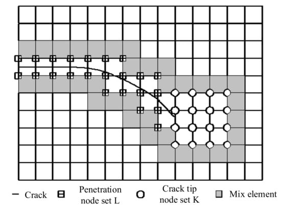
Figure 1.
Two level sets of fractures.
- (1)
- Crack penetration element:As the displacement field on both sides of the fracture surface jumps, the extended shape function [10] iswhere is the Heaviside function,The level set function [10] is:where is the element outside normal vector of the fracture at . For points not on the crack, is the shortest distance from to the crack. If the position of is consistent with the direction , take positive; conversely, take negative.
- (2)
- Crack-tip element:For elements around the crack tip, the extended shape function [10] iswhere is used to simulate the discontinuous displacement field at the crack tip. It is the basis of the Westergaard field at the asymptotic crack tip in the plane composite fracture of linear elastic fracture mechanics.
In Equation (4), only the first function is discontinuous when the crack traverses and the others are used to improve the singularity of the solution near the crack tip, where represents a local polar coordinate. The crack-tip function cannot only make the crack terminate precisely in the element, but also obtains better accuracy in the relatively rough 2D finite element mesh [29,30]. When Equation (4) is used to construct the crack-tip shape function, it can represent the geometric discontinuity and the displacement discontinuity of the elements near the fracture. The distribution state of the crack-tip displacement field can also be accurately obtained.
Based on the above two shape functions, the node displacement vector can be divided into the conventional displacement and reinforced displacement, caused by the cracks. When the Heaviside function and the asymptotic crack-tip displacement function are used to strengthen the nodes of the crack penetration element and the crack-tip element, the approximate form of the displacement vector in the XFEM discontinuous displacement mode [10] can be rewritten as follows:
where and are the finite element shape functions. , and are the node normal freedom degree and the strengthened freedom degree. I represents a set of all nodes. J represents a set of penetration element nodes. K represents a set of nodes of the crack-tip element.
In Equation (5), the first item on the right is the same as the conventional finite element method, while the second and the third are unique to the XFEM, called enhancements, to describe the existence of cracks. If there is no crack penetrating the element, the displacement field of the element will be the first term, or the first two terms if the element is penetrated, or the sum of the first and third terms when the element locates at the crack-tip. The use of and instead of and can improve the original extended finite element model, since the calculated node displacement does not need to be modified by the displacement formula.
For the strengthening node of the crack-tip branch function, if only the node of the crack-tip element is selected, the size region of the element tends to 0 and the strengthening region of the crack-tip branch function also tends to 0. In order to improve the convergence rate, the element-based reinforcement area is replaced by the geometry-based reinforcement area. Due to the close relationship between the calculation accuracy and the crack-tip position, the crack tip is suggested to be the center of a circle with radius r to eliminate the influence of the crack-tip position on the accuracy, as shown in Figure 2. The nodes in the circle are strengthened by the crack-tip function.
where S is the element area where the crack tip is located, = 3 [31].
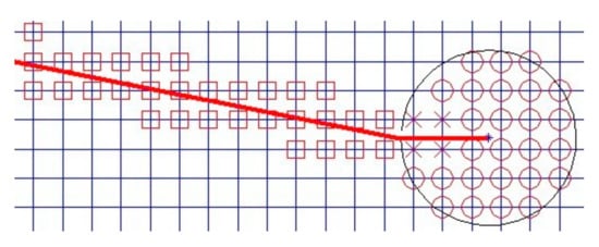
Figure 2.
Selection of the strengthening nodes.
The thick red line in Figure 2 is the crack. “□” represents the strengthening node, increasing one freedom degree in the direction of each normal freedom degree. “○” indicates the crack-tip strengthening node, increasing four freedom degrees in each direction of the normal freedom degree. “×” is the double strengthening node, increasing five freedom degrees in each direction of the normal freedom degree. Obviously, the nodes are strengthened in a large circle centered with the crack tip.
3. Propagation Simulation for the Cohesive Cracks
3.1. Governing Equation Derivation
The cohesive fracture zone is shown in Figure 3, whose calculation domain is , including the crack zone , making the displacement discontinuity on both sides. According to the stress characteristics of , it can be divided into a fracture zone (the displacement on both sides is independent and does not transfer the stress) and a cohesive zone (the displacement is discontinuous but the stress is transmitted). In Figure 3, and are the external force boundary and the displacement boundary. The stress transfer follows the constitutive law of the cohesive zone.
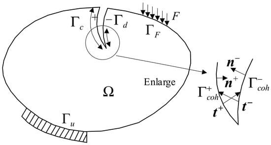
Figure 3.
Schematic diagram of the cohesive zone.
The governing equations and the boundary conditions in the region are:
where ∇ is the gradient operator, is the stress vector, is the domain of the body, is the unit outward normal vector on , is the external force, and are cohesive forces in and , and are outside normal vectors on .
Under the conditions of small strain and displacement, the kinematic equations are:
where is the strain vector, is the displacement vector and is the crack opening displacement.
The constitutive equation is:
where is the cohesive force on and is the 4th order Hooke tensor.
In order to avoid the simulation singularity, the crack tip is set at the element boundary. Assuming that the crack propagation is carried out in the element, each propagation would penetrate the crack-tip element. There are only two kinds of elements in the model: one is an ordinary element; the other is penetrated by the crack. When the mesh is subdivided and the length-width ratio of the mesh is close to 1.0, the simplified method has little effect on the calculation results. Since the displacement field of the cohesive crack tip is no longer singular, can be:
The displacement of the cohesive cracks can be:
where is the coordinate vector. , and are the element normal freedom degree vector, H function enhances the freedom vector and the crack-tip strengthened freedom degree vector, respectively. is the real displacement vector after synthesis. N is the function array. H and are the Heaviside function array and the crack-tip strengthening function array of the element nodes, respectively.
The weak form description of the problem is given to facilitate the derivation and the displacement belongs to the kinematic allowable displacement space μ.
The virtual work equation under the action of no physical force is:
where is an external force acting on the boundary.
According to the principle of the virtual work, the variation of the continuous component and the discontinuous component of the displacement mode can be obtained.
Let denote the crack opening in the global coordinate system, = , and are corresponding shape functions of the cracks and , for crack penetration elements, = N, = -N. The and of the crack-tip elements are expressed as , on both sides of the crack is equivalent, but reverse. In order to obtain the virtual work by the cohesion force, is converted to in the local coordinate through the transformation matrix M, that is .
where s is the area of one-sided crack surface on the unit length during the crack propagation, represents the crack surface cohesion and is a function of the crack opening. The incremental form can be expressed as:
where T is the material matrix and M is the transformation matrix that converts the global coordinate to the local. The incremental form of the stress and the strain is:
where , and represents strain matrices corresponding to the normal freedom degree.
Substituting Equations (17)–(19) into Equation (16), written as an incremental form, the discrete form of the governing equation is:
where:
where and represents the general part and the strengthening part of the nodes, and are the nodal internal forces, hence the right side of Equation (20) denotes the unequilibrium force of the nodes. Since the internal tensile stress of the crack is continuous, .
For the crack penetration elements:
For the crack-tip elements:
where represents corresponding strain matrix and i is the node number.
The integral load array is integrated by the element load arrays.
where is the load of the node normal freedom degrees, and are additional loads of the H function strengthening node and the crack-tip branch function strengthening node, respectively.
where , and are the distributed body force, the distributed surface force and the concentrated force, respectively.
The partial derivative of the shape function is:
In order to obtain the partial derivative of the crack-tip strengthening function in the global coordinate , the partial derivative of the crack-tip local coordinate must be firstly obtained, then the coordinate transformation is carried out as shown in Figure 4.
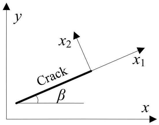
Figure 4.
Global and local coordinate systems.
According to Equations (33) and (34), the partial derivative of the crack-tip strengthening function to can be obtained as follows.
Take coordinate conversion on Equation (35) to obtain
3.2. XFEM Increment Discretization Simulation
Since concrete has obvious nonlinear fracture characteristics, the crack propagation can be simulated by the virtual crack model [32]. The nonlinear constitutive model can be used to reflect the strain softening and the extended finite element can be constructed by the presupposition virtual node method. As shown in Figure 5, the virtual node method superposes the nodes on the initial real nodes to represent the discontinuity of the fracture element.
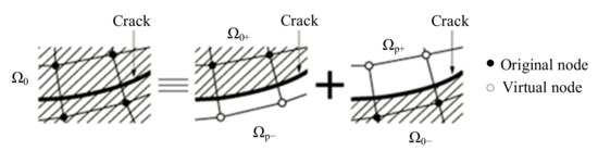
Figure 5.
Virtual node method.
In the cohesive crack model, the nonlinear closure force near the crack tip is equivalent to the virtual crack line, hence the nonlinear deformation near the crack tip can be transformed into the whole crack line. The constitutive model of the cohesive cracks describes the relationship between the nonlinear closure force in the virtual fracture zone and the relative displacement of the fracture surface. The model assumes that the macrocrack occurs when the cohesive force of the crack surface equals to 0 and the area enclosed by the distribution curve of the cohesive force in the virtual fracture zone and the coordinate axis is equal to the fracture toughness.
Due to the asymmetry of the practical structures and the bearing loads, the crack forms are diverse. Since the stress of the crack tip cannot be accurately known, the stress of the Gaussian point around the crack tip is obtained by weighted average. The weight function W is
where r represents the distance between the known node and the crack tip and l is used to control the speed of W fading from the crack tip to the known node, usually 3 times the size of the typical element.
The traction separation model is used to simulate the constitutive relationship, i.e., assuming that concrete is initially linear elastic, the initial damage and the evolution will occur after the crack is initiated. The extended element will not be damaged under the compression. According to concrete tensile tests, the nonlinear softening constitutive relationships are more consistent with the actual situations and can be used to simulate the traction separation response. When the maximum main stress at the crack tip equals the tensile strength, the introduced crack is always perpendicular to the direction of the maximum main stress. However, the crack propagation is not bound to the element boundary, it is assumed that each crack propagation needs to break through the complete element, i.e., the crack tip coincides with the element boundary to avoid the singularity simulation.
An incremental iteration process for the cohesive fracture expansion is shown in Figure 6. The key of the iterative algorithm is the expansion of new crack-tip element. The Newton–Raphson orthogonal residual method is used in the incremental load step and the energy criterion is regarded as the convergence criterion, where the strain energy of the initial elastic load step Eref stays as the convergence parameter. In order to make the crack expand smoothly, the stress iteration is added in each load increment step to ensure that the maximum main stress at the crack tip is equal to the tensile strength.
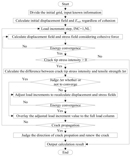
Figure 6.
The incremental iterative propagation process of cohesive cracks.
The approach to determine the length of the virtual crack zone is explained as follows. ① The initial length of the crack (including the virtual crack length) is given and the cohesive force of the crack surface is not included before initial cracking. The displacement and the opening degree of each point on the crack surface are solved. ② The iteration starts from the second step and the cohesive force at the corresponding position is calculated according to the opening degree of each point. Keep iterating to obtain the true opening degree on the crack surface until the energy convergence criterion is satisfied. ③ The exponential softening constitutive model is adopted for the relationship between the cohesive force and the crack opening, i.e., the cohesive force on the crack surface decreases exponentially with the increase of the crack opening. When the cohesive force is less than a certain value, the increase of the crack opening has little effect on it, thus a critical value of the normal cohesive force can be set. When the cohesive force is less than the value at a point, it is considered to belong to a macrocrack zone. Then the opening value of the crack tip will be the critical value of the cohesive force. Through the trial calculation, the critical value was set as 6.5 × 10² N and corresponding critical opening value was 5.25 × 10⁻⁴ mm. ④ Coordinates of the node on the crack surface corresponding to the critical opening value can be calculated through the interpolation of the opening degree of known integral nodes. The distance between the node and the virtual crack tip will be the length of the virtual fracture zone.
4. Validation and Application
4.1. Validation by the Composite Cracking Simulation
The proposed methods were validated by one-sided notched asymmetric four-point bending beam, experimental test completed in 1998 by Gálvez, etc. [33]. The numerical simulation of cracking under mixed loading of the I-II type was carried out in ABAQUS. The geometric form, loads and boundary conditions of the bending beam were shown in Figure 7. The thickness of the specimen was 50 mm, the compression strength fc was 57 MPa, the tension strength ft was 3.0 MPa, the failure energy Gf was 69 N/m and the elastic modulus E was 38 GPa.
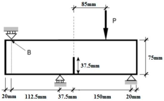
Figure 7.
Asymmetric notched four-point bending beam.
The numerical model was built as shown in Figure 8. The concrete beam adopted C3D8R element and the mesh was refined in crack propagation, support and loading point regions. The initial crack surface was preset according to the crack location in the test and there was no need to mesh the crack.
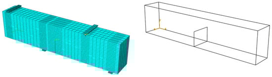
Figure 8.
Concrete beam model and initial crack location.
The initial crack module should be kept at a small distance from the beam element boundary when the model was assembled as the initial crack included in Figure 8. In order to obtain a more accurate crack propagation path, the local mesh refinement was carried out for the crack propagation region through selecting the greater stress position and the length–width ratio of the mesh was close to 1.0 to reduce the dependence of results on the mesh size. The model was loaded according to the test, controlled by the crack mouth opening displacement (CMOD), i.e., 0.004 mm/min to 40% of the peak value and 0.08 mm/min to the end of loading and the conversion of load–CMOD and load–displacement curves. Uniform load 16 MPa (P = 8 kN) was applied to the model, then the load–crack mouth opening displacement (P-CMOD) curve and the crack development path were obtained using the linear and exponential strain-softening relations on the crack surface, as shown in Figure 9. The crack propagation process was shown in Figure 10, the four-point beam notch deformed along the horizontal and vertical directions, where the I-II failure pattern was more obvious.
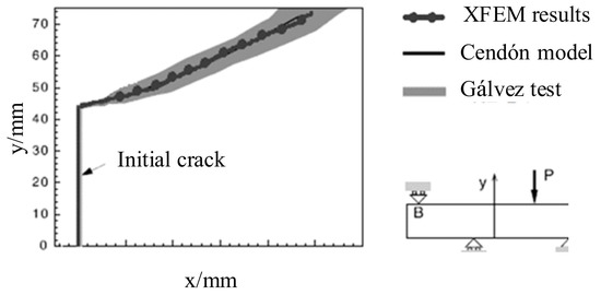
Figure 9.
Simulation results of the four-point beam.
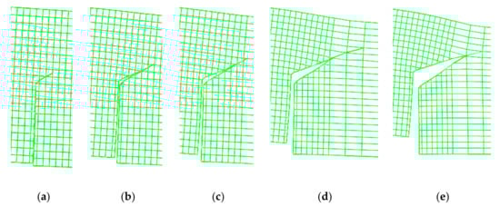
Figure 10.
Crack propagation process (250 times magnification) with different incremental steps: (a) 57 step; (b) 86 step; (c) 92 step; (d) 117 step and (e) 142 step.
The displacements of the beam notch were in agreement with test results, as shown in Figure 11. In Ref. [34], 100 pairs of nonlinear spring elements were adopted to simulate the crack along the default crack surface and multiplied the element stress by the element area to output the load according to the crack development path. In this study, the XFEM did not need to presuppose the crack path and would be more effective in practical structures.
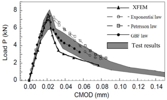
Figure 11.
Comparison of the load–crack mouth opening displacement (P-CMOD) curves.
4.2. Application on RCC Dam
The RCC gravity dam, as shown in Figure 12, located in the main stream of Tingjiang River, whose maximum dam height is 111 m, officially started construction in April 1998. The reservoir began to store water on 18 December 2000. By March 2001, dam had been completed and 51.0 × 10⁴ m3 of RCC had been poured. The elevation of the dam crest is 179.0 m, the width is 7.0 m and the total length is 308.5 m, divided into 7 dam sections. The normal storage level is 173.0 m and the design flood level is 174.76 m. The non-flow dam was taken as an example to study the expansion path of the interlayer joint. The elevation and width of the dam bottom are 80.0 m and 73.0 m, respectively. The slope ratio of the downstream surface is 1:0.75. The division of the dam concrete is shown in Figure 12, including the upstream impervious layer R180200, the parts below 120.0 m R180150 and above 120.0 m R180100.
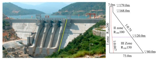
Figure 12.
The roller compacted concrete (RCC) dam and its non-flow dam section.
4.2.1. XFEM Model and Material Parameters
Due to various influence factors such as construction measures, equipment capacity, climate conditions, etc., there were defects in the plane of 40 m away from the foundation during construction, while the layer at 120 m elevation was the interface between two materials R180150 and R180100 and turned into the weakest surface among the most unfavorable layers [35,36]. The interlayer joints also easily cracked in the interfaces between the dam concrete and the foundation. Strictly speaking, each RCC layer (0.3 m thickness) should be used as a block element mesh to simulate the layered characteristics of the RCC dam, but it was bound to greatly increase the computational workload. Hence, this study only focused on the two weakest surfaces, as shown in Figure 13.
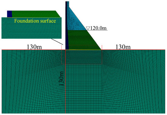
Figure 13.
Finite element computational mesh.
The modeling range of the foundation is shown in Figure 13, where the influence of the impervious curtain and the drainage holes was not considered. Fixed constraints were imposed at the bottom boundary and normal hinge constraints were imposed on the front and back boundaries. The model was primarily composed of four-node isoparametric elements. The mesh size of the local refined area was 1 m × 1 m. Convergence tests were implemented to determine the number of elements and nodes. The whole model consisted of 6762 elements and 6944 nodes, including 2533 elements in the dam body and 4229 elements in the foundation.
Mechanical parameters of dam concrete and rock mass are listed in Table 1, according to the experimental results [35]. The fracture energy is given according to the test results [37], Gf = 100 N/m.

Table 1.
Material parameters of the RCC dam.
4.2.2. Material Constitutive Relationships
The linear elastic traction–separation model was used in the dam crack area, i.e., the concrete was linear elastic in the compression and would maintain in the initial tensile stage. When the tensile stress exceeded the admissible strength, the initial damage occurred and the virtual crack model based on the XFEM would be used. The contact between crack surfaces was rigid and the separation after contact was allowed, as shown in Figure 14. The strain softening curve of the crack surface is shown in Figure 15.
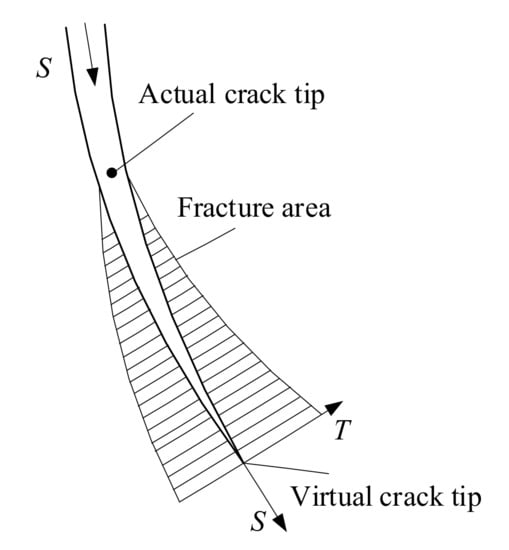
Figure 14.
Virtual crack model.
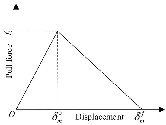
Figure 15.
Linear softening curve.
The appearance of cracks means that the cohesive force of the element begins to decline, i.e., the initial damage criterion would be the initial criterion of the crack. When the fracture criterion f reaches 1.0 (within a certain error range), a new crack will be introduced and the existed crack length will be enlarged in the next incremental step. The error range of f is:
where means the tolerance, . If , the increment step will be reduced to satisfy the initial criterion. When the maximum main stress criterion is adopted, the fracture criterion f can be:
where represents the maximum admissible main stress. The symbol is the Macauley bracket to ensure that the pure compressive strain does not damage the material. When f satisfies Equation (39), the damage occurs.
The overall average damage degree of the crack through the element boundary is denoted by D and determined by the linear criterion. For the linear softening process:
where , is the effective tractive force, indicates the fracture energy, is the effective deformation, is the maximum effective deformation during loading and is the effective deformation of a complete fracture. The normal stress and the tangential stress affected by the damage are
where and are the normal stress and the tangential stress in the case of the linear elasticity.
4.2.3. Excess Water Level Method
The imposed loads contain concrete gravity, upstream water weight, upstream water pressure, uplift pressure and seepage pressure in the joints. In order to calculate the propagation of the interlayer cracks, the excess water level method (trapezoidal overload) was used, as shown in Figure 16, increasing the water level step by step until the crack expands unsteadily.
where represents the loading water level and is the design water level.
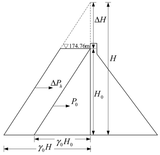
Figure 16.
The excess water level method.
4.2.4. Propagation Paths of the Interlayer Joints
The model calculation consists of four steps to ensure the accuracy and prevent the non-convergence. The initial iteration step length was 0.001, the minimum step size was 1 × 10⁻²⁰, the maximum step length was 0.1, the maximum number of the iterations was 10,000 and the nonlinear control switch was turned on in the solver. Step 1 was the initial in-situ stress equilibrium analysis to eliminate the deformation caused by the gravity action of the rock mass. The deformation was about 10−30 order of the magnitude at the end of the step. The dam gravity was imposed in step 2 and the upstream water pressure was imposed in step 3. In step 4, the water pressure was imposed on the crack surface with the magnitude of the water pressure p = γh at one end (γ is the bulk density and h is the depth of the water) and the other end 0, assuming a triangular distribution of the water pressure in the initial section of the crack surfaces. The water pressure was transformed into the equivalent joint force of the crack penetration element by the Gaussian integral [38], while the change of the seepage pressure caused by the water flow in the short crack during the propagation was ignored.
In the output of the field variables, the PHILSM (Signed distance function to describe the cracksurface, normal level set ), the PSILSM (Signed distance function to describe the initial crack front, tangential level set ) and the STATUSXFEM (Status of the XFEM element) variables were selected. The XFEM element state: the STATUSXFM value is 1.0 when the element is completely penetrated, while the value is 0.0 if there is no crack. When the element is partially broken through, the STATUSXFE value is (0.0, 1.0). Hence, the crack location can be traced in the postprocessing and whether the element is strengthened or not can be checked.
1. The weakest interlayer surface located at 120 m elevation:
The initial depth of the interlayer joint was 4 m (10% of the plane width). The XFEM calculation results show that the initiation cracking load of the weak surface was 116 m water head, about 1.17 times of the dam height, . Figure 17 shows the morphology of the interlayer crack. When the crack occurred, the fracture surface became a free surface and only the part connected to the dam body was constrained.
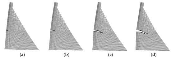
Figure 17.
Interlayer joint expansion located at 120 m elevation (magnified by 500 times). (a) Initial cracking state; (b) 49 step; (c) 148 step and (d) 181 step.
2. The weak interlayer surface located in the dam heel:
The initial depth of the interlayer joint was 2 m (2.74% of the plane width). The initiation load was 95 m water head. The crack growth pattern of the dam heel is shown in Figure 18. Figure 19 shows the gradual process of the crack propagation. The overall crack propagation trend was similar, i.e., the crack approached the horizontal at the initial stage and inclined downward to the dam bottom with the increase of the water head.
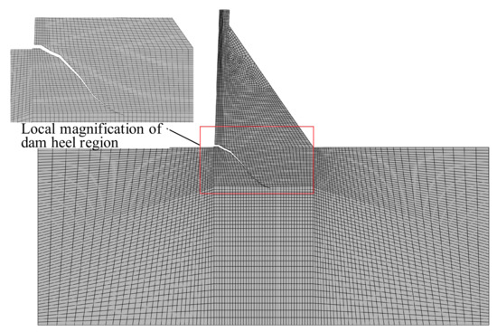
Figure 18.
Crack propagation pattern of the dam heel (magnified by 1000 times).
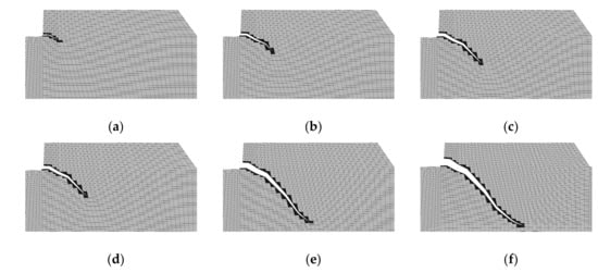
Figure 19.
Interlayer joint propagation located at the dam heel (magnified by 1000 times): (a) 39 step; (b) 110 step; (c) 211 step; (d) 370 incremental step; (e) 211 step and (f) 370 incremental step.
4.2.5. Effects of the Interlayer Joint Propagation
In order to assess the effect of the interlayer cracking on the dam structural behavior, taking the weakest surface located at the dam heel (initial crack length 2 m) for illustration, during the crack propagation, the variation of the horizontal displacement and the vertical displacement of the dam crest, the shear displacements of the interlayer joint and the opening displacement of the dam heel interlayer crack are listed in Table 2. The horizontal displacement increased obviously when the initial length of the interlayer joints extended from 2 to 3 m. Subsequently, both the horizontal displacement and the vertical displacement of the dam crest increased gradually. The shear displacement and the opening displacement increased linearly with the step-by-step propagation of the interlayer crack, basically synchronous. The measured time series of the dam crest in the recent 7 years are shown in Figure 20, where positive values represent that the dam deformed downstream and rose, otherwise it deformed upstream and sinks. The measured deformation actually includes the influence of environmental load factors such as water pressure and temperature, complex geological conditions, the influence of reservoir water permeability, etc. Although they indicate annual periodic variation of the dam horizontal and vertical deformations during normal operation, the slightly increasing trends to the downstream and the uplift should include the influence of interlayer cracks. Additionally, they will become more and more significant with the increase of the dam age.
Table 2.
The deformation of typical points during the crack propagation.
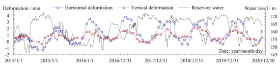
Figure 20.
The measured values of the horizontal and vertical deformation at the dam crest.
The relationships between the horizontal and the vertical displacement and the length of the interlayer joint were constructed through the polynomial regression, as shown in Figure 21. The deformation of the dam crest can be estimated from the length of the interlayer joint. When the length was 9 m, the interlayer crack extended to the curtain, at this time, the horizontal displacement was 8.3 mm and the vertical displacement was 1.29 mm. For RCC gravity dams, the further propagation of the cohesive cracks at the dam heel would damage the grouting curtain. Generally speaking, most of curtain centerlines were located at the distance from the upstream dam heel 0.06 H0–0.10 H0 (H0 is the maximum water depth, calculated from the bedrock at the normal water level), or about 0.1 times the width of the dam bottom. Therefore, the center line of the curtain was 9 m from the dam heel in the RCC dam. When the crack depth in the dam heel reached 9.73 m, it had extended to the centerline of the curtain. In this case, the penetrated water in the joint would increase the uplift pressure on the foundation surface to weaken the dam stability, thus the remedial measures must be taken to prevent the RCC dam from losing its stability during long term operation.
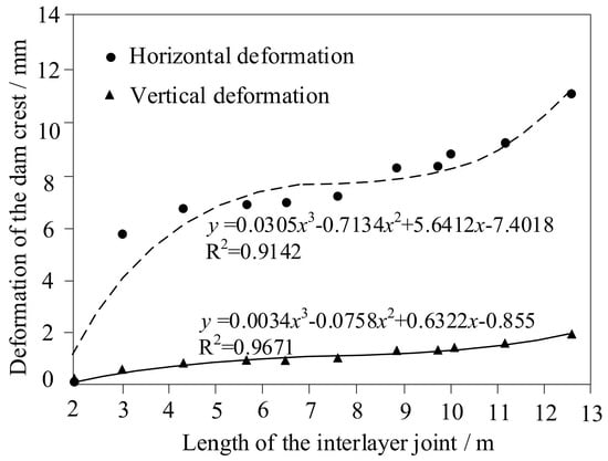
Figure 21.
Polynomial regression fitted results.
5. Conclusions
This study was devoted to evaluate the effect of cohesive crack propagation in the fragile locations of RCC dams with the XFEM. The following conclusions can be drawn.
- The established displacement function of the crack tip in the quadrilateral element and the geometric determination method of the crack-tip strengthening region were demonstrated to be more suitable for solving the cohesive cracks. The generalized Heaviside function used in the XFEM, similar to the exact local mode, could improve the adaptability of the displacement approximation function. Moreover, the adopted virtual node method could overcome the deficiency of distinguishing the type of inclined crack element by the level set.
- The computational results for the cohesive cracks through the XFEM increment discretization simulation were in agreement with the one-sided notched asymmetric four-point bending beam test results by Gálvez. In contrast to the modeling results by Cendón, the load–crack opening displacement curve and the crack development path in the loading stage were very similar. Hence, the proposed method simulating the cracking process without presupposing the crack path was proved to be feasible. The drawback is that a variable number of the freedom degrees per node are needed at the cohesive cracks in the presented method.
- The proposed methods were applied to simulate the cohesive crack propagation of the two typical weakest interlayer surfaces in the RCC gravity dam. In order to consider the influence of the plastic zone near the crack tip, the crack end was limited to the element edge and different models were used to simulate the constitutive relations. The localization caused by the softening of the crack surface could be simulated well by an overall average damage model. The gradual propagation and the morphology of the interlayer cracks obtained under the excess water level conditions indicate the crack approached the horizontal at the initial stage and inclined downward with the increase of the water head, which can make the dam deform downstream and rise.
Due to the construction technology of RCC dams, the interlayer defects are objective and unavoidable. It is vital to predict their possible propagation paths through numerical simulation for controlling the development of harmful cracks in time. Based on the regression results presented, the estimated critical values of the dam crest deformation can provide scientific support for the remedial measures to prevent the dam instability and failure during long term operation. In addition to studying the influence of single crack, the future study will focus on the stability assessment of multiple random interlayer cracks for RCC dams.
Author Contributions
Conceptualization, E.Z.; methodology, E.Z. and B.L.; software, E.Z.; validation, E.Z. and B.L.; formal analysis, E.Z.; data curation, E.Z.; writing—original draft preparation, E.Z.; writing—review and editing, E.Z. and B.L.; supervision, E.Z. All authors have read and agreed to the published version of the manuscript.
Funding
This research was funded by the National Natural Science Foundation of China (Grant Nos. 51779086, 52079046, 51739003) and the Fundamental Research Funds for the Central Universities (Grant No. B210202017).
Data Availability Statement
The data presented in this study are available in [Evaluation method for cohesive crack propagation in fragile locations of RCC dam using XFEM].
Conflicts of Interest
The authors declare no conflict of interest.
Abbreviations
The following abbreviations are used in this manuscript:
| RCC | Roller Compacted Concrete |
| XFEM | Extended Finite Element Method |
References
- Li, H.M. Analysis on and treatment of the cracks on the rolled concrete dam surface of the Fenhe reservoir two. Sci-Tech Inf. Dev. Econ. 2007, 17, 294–296. [Google Scholar]
- Zou, G.; Li, G.Z.; Wang, C.S.; Du, Z.D. Analysis on crack cause and treatment of horizontal winter construction joint. Water Conserv. Hydropower Technol. 1995, 8, 49–53. [Google Scholar]
- Qinami, A.; Bryant, E.C.; Sun, W.C.; Kaliske, M. Circumventing mesh bias by r- and h-adaptive techniques for variational eigenfracture. Int. J. Fract. 2019, 202, 129–142. [Google Scholar] [CrossRef]
- Sarrado, C.; Turon, A.; Costa, J.; Renart, J. On the validity of linear elastic fracture mechanics methods to measure the fracture toughness of adhesive joints. Int. J. Solids Struct. 2016, 81, 110–116. [Google Scholar] [CrossRef]
- Shimamoto, K.; Sekiguchi, Y.; Sato, C. Mixed mode fracture toughness of adhesively bonded joints with residual stress. Int. J. Solids Struct. 2016, 103, 120–126. [Google Scholar] [CrossRef]
- Kurumatani, M.; Soma, Y.; Terada, K. Simulations of cohesive fracture behavior of reinforced concrete by a fracture-mechanics-based damage model. Eng. Fract. Mech. 2019, 206, 392–407. [Google Scholar] [CrossRef]
- Zhang, Y.M.; Zhuang, X.Y. A softening-healing law for self-healing quasi-brittle materials: Analyzing with strong discontinuity embedded approach. Eng. Fract. Mech. 2018, 192, 290–306. [Google Scholar] [CrossRef]
- Rukavishnikov, V.A.; Mosolapov, A.O.; Rukavishnikova, E.I. Weighted finite element method for elasticity problem with a crack. Comput. Struct. 2021, 243, 106400. [Google Scholar] [CrossRef]
- Belytschko, T.; Black, T. Elastic crack growth in finite elements with minimal remeshing. Int. J. Numer. Methods Eng. 1999, 45, 601–620. [Google Scholar] [CrossRef]
- Moës, N.; Dolbow, J.; Belytschko, T. A finite element method for crack growth without remeshing. Int. J. Numer. Methods Eng. 1999, 45, 131–150. [Google Scholar] [CrossRef]
- Tran, T.D.; Le, C.V. Extended finite element method for plastic limit load computation of cracked structures. Int. J. Numer. Methods Eng. 2015, 104, 2–17. [Google Scholar] [CrossRef]
- Aghajanzadeh, S.M.; Mirzabozorg, H. Concrete fracture process modeling by combination of extended finite element method and smeared crack approach. Theor. Appl. Fract. Mech. 2019, 101, 306–319. [Google Scholar] [CrossRef]
- Surendran, M.; Natarajan, S.; Palani, G.S.; Bordas, S.P.A. Linear smoothed extended finite element method for fatigue crack growth simulations. Eng. Fract. Mech. 2019, 206, 551–564. [Google Scholar] [CrossRef]
- Kyoungsoo, P.; Paulino, G.H. Cohesive zone models: A critical review of traction-separation relationships across fracture surfaces. Appl. Mech. Rev. 2013, 64, 1–20. [Google Scholar]
- Moës, N.; Belytschko, T. Extended finite element method for cohesive crack growth. Eng. Fract. Mech. 2002, 69, 813–833. [Google Scholar] [CrossRef]
- Wolff, K.P.; Pitangueira, R.L.S.; Peixoto, R.G. A displacement-based and explicit non-planar 3D crack propagation model in the generalized/extended finite element method. Theor. Appl. Fract. Mech. 2020, 108, 102647. [Google Scholar] [CrossRef]
- Yan, Z.; Feng, W.J.; Zhang, C.; Liu, J.X. The extended finite element method with novel crack-tip enrichment functions for dynamic fracture analysis of interfacial cracks in piezoelectric–piezomagnetic bi-layered structures. Comput. Mech. 2019, 64, 1303–1319. [Google Scholar] [CrossRef]
- Remmers, J.J.C.; de Borst, R.; Needleman, A. A cohesive segments method for the simulation of crack growth. Comput. Mech. 2003, 31, 69–77. [Google Scholar] [CrossRef]
- Sanchez-Rivadeneira, A.G.; Duarte, C.A. A simple, first-order, well-conditioned, and optimally convergent Generalized/eXtended FEM for two- and three-dimensional linear elastic fracture mechanics. Comput. Methods Appl. Mech. Eng. 2020, 372, 113388. [Google Scholar] [CrossRef]
- Zhao, J.W.; Feng, S.Z.; Tao, Y.R.; Li, Z.X. Stable node-based smoothed extended finite element method for fracture analysis of structures. Comput. Struct. 2020, 240, 106357. [Google Scholar] [CrossRef]
- Jiang, S.Y.; Du, C.B. Study on dynamic interaction between crack and inclusion or void by using XFEM. Struct. Eng. Mech. 2017, 63, 329–345. [Google Scholar]
- Liu, W.H.; Zhang, L.W. A novel XFEM cohesive fracture framework for modeling nonlocal slip in randomly discrete fiber reinforced cementitious composites. Comput. Methods Appl. Mech. Eng. 2019, 355, 1026–1061. [Google Scholar] [CrossRef]
- Nguyen, N.V.; Lee, D.; Nguyen-Xuan, H.; Lee, J. A polygonal finite element approach for fatigue crack growth analysis of interfacial cracks. Theor. Appl. Fract. Mech. 2020, 108, 102576. [Google Scholar] [CrossRef]
- Alfano, G.; Marfia, S.; Sacco, E. A cohesive damage-friction interface model accounting for water pressure on crack propagation. Comput. Methods Appl. Mech. Eng. 2006, 196, 192–209. [Google Scholar] [CrossRef]
- Zhang, S.R.; Wang, G.H.; Yu, X.R. Seismic cracking analysis of concrete gravity dams with initial cracks using the extended finite element method. Eng. Struct. 2013, 56, 528–543. [Google Scholar] [CrossRef]
- Jiang, S.Y.; Du, C.B. Coupled finite volume methods and extended finite element methods for the dynamic crack propagation modelling with the pressurized crack surfaces. Shock. Vib. 2017, 3751340. [Google Scholar] [CrossRef]
- Zhao, K.K.; Jiang, P.F.; Feng, Y.J.; Sun, X.D.; Cheng, L.X.; Zheng, J.W. Numerical investigation of hydraulic fracture propagation in naturally fractured reservoirs based on lattice spring model. Geofluids 2020, 2020, 8845990. [Google Scholar] [CrossRef]
- Haghani, M.; Neya, B.N.; Ahmadi, M.T.; Amiri, J.V. Combining XFEM and time integration by alpha-method for seismic analysis of dam-foundation-reservoir. Theor. Appl. Fract. Mech. 2020, 109, 102752. [Google Scholar] [CrossRef]
- Martínez-Pañeda, E.; Natarajan, S.; Bordas, S. Gradient plasticity crack tip characterization by means of the extended finite element method. Comput. Mech. 2017, 59, 831–842. [Google Scholar] [CrossRef]
- Huan, S.L.; Kee, B.Y. Estimation of C(t) and the creep crack tip stress field of functionally graded materials and verification via finite element analysis. Compos. Struct. 2016, 153, 728–737. [Google Scholar]
- Stolarska, M.; Chopp, D.L.; Moës, N.; Belytschko, T. Modelling crack growth by level sets in the extended finite element method. Int. J. Numer. Methods Eng. 2001, 51, 943–960. [Google Scholar] [CrossRef]
- Montoya, A.; Ramirez-Tamayo, D.; Millwater, H.; Kirby, M. A complex-variable virtual crack extension finite element method for elastic-plastic fracture mechanics. Eng. Fract. Mech. 2018, 202, 242–258. [Google Scholar] [CrossRef]
- Gálvez, J.C.; Elices, M.; Guinea, G.V.; Planas, J. Mixed mode fracture of concrete under proportional and nonproportional loading. Int. J. Fract. 1998, 94, 267–284. [Google Scholar] [CrossRef]
- Cendón, D.A.; Gálvez, J.C.; Elices, M.; Planas, J. Modeling the fracture of concrete under mixed loading. Int. J. Fract. 2000, 103, 293–310. [Google Scholar] [CrossRef]
- Li, Q.X.; Dong, Q.J.; Mao, Y.Q. Design of RCC gravity dam of Mianhuatan hydropower station. Water Power 2001, 7, 24–27. [Google Scholar]
- Wang, S.C.; Chen, H.C. RCC dam construction of Mianhuatan hydropower station. Water Power 2001, 7, 41–44. [Google Scholar]
- Zhang, C.H.; Wang, G.L.; Wang, S.M.; Dong, Y.X. Experimental tests of rolled compacted concrete and nonlinear fracture analysis of rolled compacted concrete dams. J. Mater. Civil. Eng. 2002, 14, 108–115. [Google Scholar]
- Sheng, M.; Li, G.S. Extended finite element modeling of hydraulic fracture propagation. Eng. Mech. 2014, 31, 123–128. [Google Scholar]


Publisher’s Note: MDPI stays neutral with regard to jurisdictional claims in published maps and institutional affiliations. |
© 2020 by the authors. Licensee MDPI, Basel, Switzerland. This article is an open access article distributed under the terms and conditions of the Creative Commons Attribution (CC BY) license (http://creativecommons.org/licenses/by/4.0/).