Macroscopic Lattice Boltzmann Method


Department of Computing and Mathematics, Manchester Metropolitan University, Manchester M1 5GD, UK
Water 2021, 13(1), 61; https://doi.org/10.3390/w13010061
Submission received: 15 November 2020
/
Revised: 24 December 2020
/
Accepted: 25 December 2020
/
Published: 30 December 2020
(This article belongs to the Section Hydraulics and Hydrodynamics)
Abstract
:The lattice Boltzmann method (LBM) is a highly simplified model for fluid flows using a few limited fictitious particles. It has been developed into a very efficient and flexible alternative numerical method in computational physics, demonstrating its great power and potential for resolving more and more challenging physical problems in science and engineering covering a wide range of disciplines such as physics, chemistry, biology, material science and image analysis. The LBM is implemented through the two routine steps of streaming and collision using the three parameters of the lattice size, particle speed and collision operator. A fundamental question is if the two steps are integral to the method or if the three parameters can be reduced to one for a minimal lattice Boltzmann method. In this paper, it is shown that the collision step can be removed and the standard LBM can be reformulated into a simple macroscopic lattice Boltzmann method (MacLAB). This model relies on macroscopic physical variables only and is completely defined by one basic parameter of the lattice size , bringing the LBM into a precise “lattice” Boltzmann method. The viscous effect on flows is naturally embedded through the particle speed, making it an ideal automatic simulator for fluid flows. Three additional advantages compared to the existing LBMs are that: (i) physical variables can directly be retained as the boundary conditions; (ii) much less computational memory is required; and (iii) the model is unconditionally stable. The findings are demonstrated and confirmed with numerical tests including flows that are independent of and dependent on fluid viscosity, 2D and 3D cavity flows and an unsteady Taylor–Green vortex flow. This provides an efficient and powerful model for resolving physical problems in various disciplines of science and engineering.
Keywords:
macroscopic lattice Boltzmann method; fluid flows; computational fluid dynamics; numerical methodPACS:
47.11.-j; 02.60.Cb; 02.70.-c1. Introduction
The birth of the lattice Boltzmann method (LBM) fulfils a dream that simple arithmetic calculations can simulate complex fluid flows without solving complicated partial differential flow equations. The method is a highly simplified discrete model for fluid flows using a few limited fictitious particles that move one grid at a constant time interval and collide with each other at a grid point on uniform lattices, which are the two routine steps for the implementation of the method to simulate fluid flows. As such, a real complex particle dynamics is approximated as a regular particle model using three parameters of the lattice size, particle speed and collision operator. The LBM is characterised by its simplicity, parallel processing and easy treatment of boundary conditions [1]. The first fully discrete model for fluid flows on a square lattice was proposed by Hardy et al. [2] in 1976. Ten years later, Frisch et al. [3] for the first time obtained a correct lattice gas automata (LGA) for Navier–Stokes equations using a six-velocity hexagonal lattice. The LGA is comprised of two steps: streaming and collision. The two steps are represented by the lattice size, particle speed and a collision operator on a uniform lattice. In physics, the former and the latter simulate the phenomena of fluid movement and diffusion, respectively, which determine the basic feature of an LGA. Often, simulations generated using an LGA are very noisy due to its Boolean variable with one for the presence and zero for the absence of particles at a lattice point [4,5]. Furthermore, the numerical procedure involves the calculations of particle probability, which reduces the efficiency of the model. To overcome these, the lattice Boltzmann method was proposed [6], and its basic difference from the LGA is that the Boolean variable is replaced with a particle distribution function. Such an approach eliminates the statistical noise in an LGA and retains all the advantages of locality in the kinetic form of an LGA [1]. McNamara and Zanetti [6] first used the lattice Boltzmann method as an alternative to the LGA in 1988. As the collision operator takes a complex matrix form, this prevents the LBM from becoming a competing numerical method. A breakthrough in progress was made by Higuera and Jiménez [7] through linearisation of the collision term around its local equilibrium state. This greatly simplifies the collision operator. Noble et al. [8] used this idea to express the collision operator as , in which is the particle distribution function; is the local equilibrium distribution function; and is a collision matrix. Later, several researchers [9,10] suggested a simple linearized form for the collision matrix by using a single time relaxation towards the local equilibrium distribution, , which is popularly known as the Bhatnagar–Gross–Krook (BGK) collision operator [11], where is the Kronecker delta function taking one when , or otherwise zero, and is called the single relaxation time that takes a value. The correct choice of together with the lattice size and time step can achieve a desired fluid viscosity. This leads to the single relaxation time lattice Boltzmann method (SRT LBM), which has been the most efficient and used so far,
where is a lattice coordinate along the j-axis in the Cartesian coordinate system, i.e., in the two-dimensional space; t is time; is the component of the particle velocity vector in -link of the lattice and defined by time step and lattice size , e.g., when for nine particles moving in the two-dimensional uniform square lattice (D2Q9), in which e is the particle speed and defined as ; and is the local equilibrium distribution function given by:
in which is the fluid density and is a weighting factor depending on the lattice pattern, e.g., when , when and when on D2Q9. After the distribution function is calculated from the lattice Boltzmann Equation (1), the macroscopic psychical variables, density and velocity are simply updated as:
Since then, the study of the lattice Boltzmann method and the applications of the method have received extensive attentions, making it become a very powerful modelling tool in many areas such as thermodynamics [12], aerodynamics [13], multiphase flows [14], turbulent flows [15], hemodynamics [16], biomechanics [17], image analysis [18], biology [19] and environmental science [20].
In applications, it is found that the SRT LBM suffers from a numerical instability. To remedy this, the multiple relaxation time (MRT) collision operator was introduced in 1992 [21,22]. This improves the stability, but it reduces the efficiency. To accelerate the simulation, a two relaxation time collision operator was developed in 2008 [23], which has almost the same efficiency as the SRT LBM. As research progresses, it is noticed that MRT or TRT still suffers from numerical instabilities when fluid flows with very small viscosity are simulated. After realising that this is caused by an insufficient degree of Galilean invariance in the collision step, Geier et al. [24] proposed a cascaded lattice Boltzmann method by relaxing the particle distribution function to its local equilibrium state in the central moment space, making the LBM stable for simulating flows with small viscosity close to zero. In 2015, Geier et al. [25] further improved their central moment LBM using the cumulant in collision operator, which is called the cumulant lattice Boltzmann method (CLBM). Despite such enhancements, these schemes are more complicated and less efficient due to a manipulation of the matrices. In addition, these schemes share the same drawback as the existing LBM in that the boundary conditions for a physical variable such as velocity cannot be implemented without being converted to particle distribution functions, which further reduces the efficiency and accuracy of the methods. Recently, Chen et al. [26] developed a simplified lattice Boltzmann method without the evolution of the particle distribution function, which successfully removes this drawback and enables the direct use of a physical variable as the boundary conditions. However, the method involves the two steps of the predictor and corrector, which is more complicated than the SRT LBM. Nevertheless, through all this research, the LBM has greatly been improved and developed to a point where it has become a very efficient and flexible alternative numerical method in computational physics. Its potential power is much beyond the original scope, being explored and demonstrated in various disciplines of science and engineering with time [27,28,29,30].
2. Macroscopic Lattice Boltzmann Model
The above literature review highlights that the major research to improve the method has been carried out on the collision operator for resolving the well-known instability problem in the SRT LBM since 1992, leading to four representative variants of the method, MRT, TRT, central moment and cumulant LBMs. Even so, choosing suitable parameters or values for the collision operators is not clear, and they cannot be tuned without using trial and error during simulations, which becomes more complicated in a non-single relaxation time scheme due to its complexity. This unnecessarily wastes time and computing resource, and it may become awkward to simulate a large-scale flow system, preventing the LBM from becoming an automatic simulator for any scale flows when a super-fast computer such as a quantum computer becomes available one day. As the central problem comes from the collision operator, such a problem may be resolved forever if the collision operator can be removed. Since the function of the collision is to relax the distribution function towards its local equilibrium state, it may be removed and replaced with the local equilibrium distribution function by setting in Equation (1). Following this idea, after mathematical manipulations, we obtain the following simple macroscopic lattice Boltzmann model (MacLAB),
to determine the physical density and velocity directly from the local equilibrium distribution function without calculating the distribution function using Equation (1) unlike existing LBMs (the theoretical derivation is given in Section 3). Apparently, the model involves the local equilibrium distribution function only. However, doing so brings a new problem of how to consider the fluid viscosity in the absence of the collision step. We overcome this from the finding, through the recovery of the Navier–Stokes equations from Equations (4) and (5), that if the particle speed e is determined using:
which is employed in Equation (2) instead of using to calculate the local equilibrium distribution function , the flow viscosity is naturally taken into account in the model. In the MacLAB, once a lattice size is chosen, the model is ready to simulate a flow with a viscosity because stands for a neighbouring lattice point; at time of represents its known quantity at the current time; and the particle speed e is determined from Equation (6) for use in the computation of . In addition, the time step is no longer an independent parameter and needs to be determined as , which is used in the simulations of unsteady flows. Consequently, only the lattice size is required in the MacLAB for the simulation of fluid flows, bringing the LBM into a precise “lattice” Boltzmann method. This enables the model to become an automatic simulator for any scale flows without tuning other simulation parameters, making it possible and easy to model a large flow system when a super-fast computer such as a quantum computer becomes available in the future. The model is unconditionally stable as it shares the same valid condition as that for , or the Mach number is much smaller than one, in which is a characteristic flow speed. The Mach number can also be expressed as a lattice Reynolds number of via Equation (6). In practical simulations, it is found that the model is stable if where is the maximum flow speed and is used as the characteristic flow speed. The main features are that there is no collision operator and only macroscopic physical variables such as the density and velocity are required, which are directly retained as boundary conditions with a minimum memory requirement. The implementation of the model starting from the initial density and velocity is to (i) choose the lattice size and determine the particle speed e from Equation (6), (ii) calculate from Equation (2) using the density and velocity, (iii) update the density and velocity using Equations (4) and (5), (iv) apply the boundary conditions, and (v) repeat Step (ii) until a solution is reached. The only limitation of the described model is that, for very small viscosity or high speed flow, the chosen lattice size after satisfying may turn out to generate very large lattice points (lattice points, e.g., for one dimension with a length of L are calculated as , and is the lattice points); if the total lattice points are too big such that the demanding computations are beyond the current power of a computer, the simulation cannot be carried out. Such difficulties may be solved or relaxed through parallel computing using computer techniques such as GPU processors and multiple servers and will be largely or completely removed using quantum computing when a quantum computer becomes available.
3. Recovery of the Navier–Stokes Equations
Taking ∑ Equation (8) and Equation (8) yields:
and:
respectively. In the lattice Boltzmann method, the density and velocity are determined using the distribution function as:
Combining Equation (11) with Equations (9) and (10) results in the current MacLAB, Equations (4) and (5). Since the local equilibrium distribution function has the features of:
with reference to Equation (11), the following relationships,
hold, which are the conditions that retain the conservation of the mass and momentum in the lattice Boltzmann method.
Next, we prove that the continuity and Navier–Stokes equations can be recovered from Equations (4) and (5). Rewriting Equation (1) as:
Apparently, when , the above equation becomes Equation (8), which leads to Equations (4) and (5); hence, Equation (14) is a general equation and is used in the following derivation. Applying a Taylor expansion to the two terms on the right-hand side of Equation (14) in time and space at point yields:
and:
According to the Chapman–Enskog analysis, can be expanded around :
After substituting Equations (15)–(17) into Equation (14), equating the coefficients of with various orders results for the order in:
for the order in:
and for the order in:
Now, taking ∑Equation (23) leads to:
as:
due to the condition of the conservation of mass and momentum Equation (13). Evaluating the terms in the above equation using Equation (2) produces the exact continuity equation,
Multiplying Equation (23) by provides:
Taking ∑ Equation (27) leads to:
under the same condition (25) as that in the derivation of Equation (24). Evaluating the terms in the above equation using Equation (2) produces the exact momentum equation, the Navier–Stokes equation at second-order accuracy on the condition that the Mach number ,
where pressure p is defined as:
and the kinematic viscosity is:
4. Numerical Tests
In order to demonstrate the validation of the described model, five numerical simulations were carried out using D2Q9 and D3Q19 lattices for 2D and 3D flows, respectively. For D3Q19, the particle velocity vector is , and the weighting factor for Equation (2) is when , when and when . Physical variables in SI units without explicit notation are used in the numerical simulations, e.g., the density implies kg/m3.
4.1. Couette Flow
The first test is a Couette flow through two parallel plates without a pressure gradient. The distance between the plates is . The top plate moves at a velocity of in the streamwise direction, and the bottom plate is fixed. If x stands for the streamwise direction and y for the vertical direction, the analytical solution is:
which is the same test as that used by Chen et al. [26]. This is a very interesting case as the steady flow is independent of the flow viscosity according to the theory (32). We use and lattices in the x and y directions for three simulations of flows with three kinematic viscosities of and , respectively. The periodic boundary conditions are applied at the inflow and outflow boundaries. After the steady solutions are reached, the results are indeed independent of the viscosities, and one of those is shown in Figure 1, demonstrating excellent agreement with the analytical solution.
4.2. Couette Flow with a Pressure Gradient
The second test is the same flow as that in Test 1 except that a pressure gradient of is specified, which is added to the right-hand side of Equation (5) as [31]. Both plates are fixed with zero velocities at the top and bottom boundaries at which no calculations are needed. The flow is affected by viscosity, and the analytical solution is:
The flow is simulated using three viscosities of and . The numerical results are plotted in Figure 2, showing the effect of viscosity on the flow, in excellent agreement with the analytical solutions. This confirms the unique feature that the current model can simulate viscous flow correctly due to the use of Equation (6), although no explicit effect of viscosity on flows is taken into account.
4.3. 2D Cavity Flow
The third test is a 2D cavity flow, which is a well-known complex flow within a simple geometry. The domain is a square. The boundary conditions are that the top lid moves at a velocity of and with ; the other three sides are fixed, or no slip boundary condition is applied, i.e., and . The Reynolds number . We use or lattices in the simulation, which is carried out on the inside of the cavity excluding the four sides where the velocities are retained as boundary conditions. After the steady solution is obtained, the flow pattern in the velocity vectors is shown in Figure 3, which closely agrees with the well-known study by Ghia et al. [32]. The results are further compared against their numerical solutions for velocity profiles of and along the y and x directions through the geometric centre of the cavity in Figure 4 and Figure 5, respectively, demonstrating very good agreements.
4.4. 2D Taylor–Green Vortex
The fourth test is a 2D Taylor–Green vortex. This is an unsteady flow driven by decaying vortexes for which there is an exact solution of the incompressible Navier–Stokes equations, and it is often applied to the validation of a numerical method for the solution to the incompressible Navier–Stokes equations. The initial conditions are and . The analytical solutions are and . The time for an unsteady flow from the initial state is accumulated by its increase with time step . We use or lattices for a square domain of with a kinematic viscosity of and , which gives the Reynolds number of . The periodic boundary conditions are used. The simulation is run for the total time of 30 s. The velocity field is plotted in Figure 6, showing the correct flow pattern. The velocity profiles for at and at along the y direction are depicted and compared with the analytical solutions in Figure 7, showing excellent agreements and confirming the accuracy of the method for an unsteady flow.
4.5. 3D Cavity Flow
The final test is a 3D cavity flow. This is again a well-known complex flow involving 3D vortices within a simple cube with dimensions of in streamwise direction x, spanwise direction y and vertical direction z. No-slip boundary conditions, i.e, , and , are applied to five fixed sides except for the top lid, where , and with are specified. The Reynolds number is . or total lattices of are used, and the simulation is undertaken only within the cube, excluding the boundaries where the velocities are retained. After the steady solution is reached, the flow characterises are displayed through the two-dimensional planar projections of the velocity vector field on the x-z, y-z and x-y centroidal planes of the cube in Figure 8, Figure 9 and Figure 10, respectively, demonstrating flow patterns in good agreement with those by Wong and Baker [33]. In addition, the distribution of the velocity component on the vertical plane centerline is widely used as a 3D lid-driven cavity benchmark test. We compare this velocity component against the results by Wong and Baker [33] and also by Jiang et al. [34] in Figure 11, showing good agreements.
5. Conclusions
A novel macroscopic lattice Boltzmann method (MacLAB) for the Navier–Stokes equations is proposed and validated. It can accurately simulate fluid flows using only the lattice size, bringing the LBM into a precise lattice Boltzmann method and revolutionising the standard LBM theory. This takes the research on the method into a new era in which future work may focus on improving the accuracy of or formulating a new local equilibrium distribution function. The particle speed is determined through the viscosity and lattice size, and the time step is calculated as . The model is unconditional stable as long as the valid condition for the local equilibrium distribution function holds. When a super-fast computer such as a quantum computer becomes available in the future, this will enable the MacLAB to take any fine lattice to simulate most challenging fluid flows such as turbulent flows without relying on a turbulent flow model. All these make the method an automatic simulator for fluid flows in all relevant problems. The method is straightforward to extend for resolving other physical problems in different disciplines such as chemical and environmental engineering.
Funding
This research received no external funding.
Institutional Review Board Statement
Not applicable.
Informed Consent Statement
Not applicable.
Data Availability Statement
Not applicable.
Conflicts of Interest
The author declares no conflict of interest.
References
- Chen, S.; Doolen, G.D. Lattice Boltzmann Method for Fluid Flows. Annu. Rev. Fluid Mech. 1998, 30, 329–364. [Google Scholar] [CrossRef] [Green Version]
- Hardy, J.; de Pazzis, O.; Pomeau, Y. Molecular dynamics of a classical lattice gas: Transport properties and time correlation functions. Phys. Rev. A 1976, 13, 1949–1961. [Google Scholar] [CrossRef]
- Frisch, U.; Hasslacher, B.; Pomeau, Y. Lattice-Gas Automata for the Navier–Stokes Equation. Phys. Rev. Lett. 1986, 56, 1505–1508. [Google Scholar] [CrossRef] [Green Version]
- Chopard, B.; Droz, M. Cellular Automata Modeling of Physical Systems; Cambridge University Press: Cambridge, UK, 1998. [Google Scholar]
- Rivet, J.P.; Boon, J.P. Lattice Gas Hydrodynamics; Cambridge University Press: Cambridge, UK, 2001. [Google Scholar]
- McNamara, G.R.; Zanetti, G. Use of the Boltzmann equation to simulate lattice-gas automata. Phys. Rev. Lett. 1988, 61, 2332–2335. [Google Scholar] [CrossRef]
- Higuera, F.; Jiménez, J. Boltzmann approach to lattice gas simulations. Eur. Lett. 1989, 9, 663–668. [Google Scholar] [CrossRef]
- Noble, D.R.; Chen, S.; Georgiadis, J.G.; Buckius, R.O. A consistent hydrodynamic boundary condition for the lattice Boltzmann method. Phys. Fluids 1995, 7, 203–209. [Google Scholar] [CrossRef]
- Qian, Y.H. Lattice Gas and Lattice Kinetic Theory Applied to the Navier–Stokes Equations. Ph.D. Thesis, Université Pierre et Marie Curie, Paris, France, 1990. [Google Scholar]
- Chen, S.; Chen, H.D.; Martinez, D.; Matthaeus, W. Lattice Boltzmann model for simulation of magnetohydrodynamics. Phys. Rev. Lett. 1991, 67, 3776–3779. [Google Scholar] [CrossRef]
- Bhatnagar, P.L.; Gross, E.P.; Krook, M. A model for collision processes in gases. I: Small amplitude processes in charged and neutral one-component system. Phys. Rev. 1954, 94, 511–525. [Google Scholar] [CrossRef]
- Zarghami, A.; den Akker, H.E.A.V. Thermohydrodynamics of an evaporating droplet studied using a multiphase lattice Boltzmann method. Phys. Rev. E 2017, 95, 043310. [Google Scholar] [CrossRef] [Green Version]
- Mohamad, H.H.; Masoud, M. Continuous and Discrete Adjoint Approach Based on Lattice Boltzmann Method in Aerodynamic Optimization Part I: Mathematical Derivation of Adjoint Lattice Boltzmann Equations. Adv. Appl. Math. Mech. 2014, 6, 570–589. [Google Scholar]
- Shan, X.; Chen, H. Lattice Boltzmann model for simulating flows with multiple phases and components. Phys. Rev. E 1993, 47, 1815–1819. [Google Scholar] [CrossRef] [Green Version]
- Chen, H.; Kandasamy, S.; Orszag, S.; Shock, R.; Succi, S.; Yakhot, V. Extended Boltzmann Kinetic Equation for Turbulent Flows. Science 2003, 301, 633–636. [Google Scholar] [CrossRef]
- Golbert, D.R.; Blanco, P.J.; Clausse, A.; Feijóo, R.A. Tuning a lattice-Boltzmann model for applications in computational hemodynamics. Med. Eng. Phys. 2012, 34, 339–349. [Google Scholar] [CrossRef]
- Javed, S.; Sohail, A.; Maqbool, K.; Butt, S.I.; Chaudhry, Q.A. The Lattice Boltzmann method and computational analysis of bone dynamics-I. Complex Adapt. Syst. Model. 2017, 5, 1–14. [Google Scholar] [CrossRef] [Green Version]
- Chen, J.; Chai, Z.; Shi, B.; Zhang, W. Lattice Boltzmann method for filtering and contour detection of the natural images. Comput. Math. Appl. 2014, 68, 257–268. [Google Scholar] [CrossRef]
- Finck, M.; Hänel, D.; Wlokas, I. Simulation of nasal flowby lattice Boltzmann methods. Comput. Biol. Med. 2007, 37, 739–749. [Google Scholar] [CrossRef]
- Zhou, J.G.; Haygarth, P.M.; Withers, P.J.A.; Macleod, C.J.A.; Falloon, P.D.; Beven, K.J.; Ockenden, M.C.; Forber, K.J.; Hollaway, M.J.; Evans, R.; et al. Lattice Boltzmann method for the fractional advection-diffusion equation. Phys. Rev. E 2016, 93, 043310. [Google Scholar] [CrossRef] [Green Version]
- d’Humières, D. Generalized lattice Boltzmann equations. In Rarefied Gas Dynamics: Theory and Simulations, Progress in Astronautics and Aeronautics; Shizgal, B.D., P.Weaver, D., Eds.; 1992; Volume 159, pp. 450–458. [Google Scholar]
- Lallemand, P.; Luo, L.S. Theory of the lattice Boltzmann method: Dispersion, dissipation, isotropy, Galilean invariance, and stability. Phys. Rev. E 2000, 61, 6546–6562. [Google Scholar] [CrossRef] [Green Version]
- Ginzburg, I.; Verhaeghe, F.; d’Humières3, D. Two-Relaxation-Time Lattice Boltzmann Scheme: About Parametrization, Velocity, Pressure andMixed Boundary Conditions. Commun. Comput. Phys. 2008, 3, 427–478. [Google Scholar]
- Geier, M.; Greiner, A.; Korvink, J.G. Cascaded digital lattice Boltzmann automata for high Reynolds number flow. Phys. Rev. E 2006, 73, 066705. [Google Scholar] [CrossRef]
- Geier, M.; Schönherr, M.; Pasquali, A.; Krafczyk, M. The cumulant lattice Boltzmann equation in three dimensions: Theory and validation. Comput. Math. Appl. 2015, 70, 507–547. [Google Scholar] [CrossRef] [Green Version]
- Chen, Z.; Shu, C.; Wang, Y.; Yang, L.M.; Tan, D. A Simplified Lattice Boltzmann Method without Evolution of Distribution Function. Adv. Appl. Math. Mech. 2017, 9, 1–22. [Google Scholar] [CrossRef]
- Succi, S. The Lattice Boltzmann Equation for Fluid Dynamics and Beyond; Oxford University Press: Oxford, UK, 2001. [Google Scholar]
- Wolf-Gladrow, D. Lattice-Gas Cellular Automata and Lattice Boltzmann Models; Springer: Berlin/Heidelberg, Germany, 2000. [Google Scholar]
- Guo, Z.L.; Shu, C. Lattice Boltzmann Method and Its Applications in Engineering; World Scientific Publishing: Singapore, 2013. [Google Scholar]
- Krüger, T.; Kusumaatmaja, H.; Kuzmin, A.; Shardt, O.; Silva, G.; Viggen, E.M. The Lattice Boltzmann Method: Principles and Practice; Springer: Berlin, Germany, 2017. [Google Scholar]
- Zhou, J.G. Lattice Boltzmann Methods for Shallow Water Flows; Springer: Berlin, Germany, 2004. [Google Scholar]
- Ghia, U.; Ghia, K.; Shin, C. High-Re Solutions for Incompressible Flow Using the Navier–Stokes Equations and a Multigrid Method. J. Comput. Phys. 1982, 48, 387–411. [Google Scholar] [CrossRef]
- Wong, K.L.; Baker, A.J. A 3D incompressible Navier–Stokes velocity-vorticity weak form finite element algorithm. Int. J. Numer. Methods Fluids 2002, 38, 99–123. [Google Scholar] [CrossRef]
- Jiang, B.N.; Lin, T.L.; Povinelli, L.A. Large scale computation of incompressible viscous flows by least-squares finite element method. Comput. Methods Appl. Mech. Eng. 1994, 114, 213–231. [Google Scholar] [CrossRef] [Green Version]
Figure 1.
Couette flow through two parallel plates without a pressure gradient. The distance between the plates is . The top plate moves at a velocity of in the streamwise direction, and the bottom plate is fixed, where no calculations are required at the top or bottom boundaries. The periodic boundary conditions are applied at the inflow and outflow boundaries. is used for three simulations of flows with three kinematic viscosities of and , respectively. All the steady numerical results are almost identical and are independent of flow viscosity, as shown here in the comparison of one numerical result with the analytical solution. MacLAB, macroscopic lattice Boltzmann method.

Figure 2.
Couette flow through two parallel plates under a pressure gradient of . The distance between the plates is . Both plates are fixed with zero velocities at the top and bottom boundaries, where no calculations are needed. The steady numerical results are dependent on flow viscosity and shown in this figure through simulations of flows with three viscosities of and .
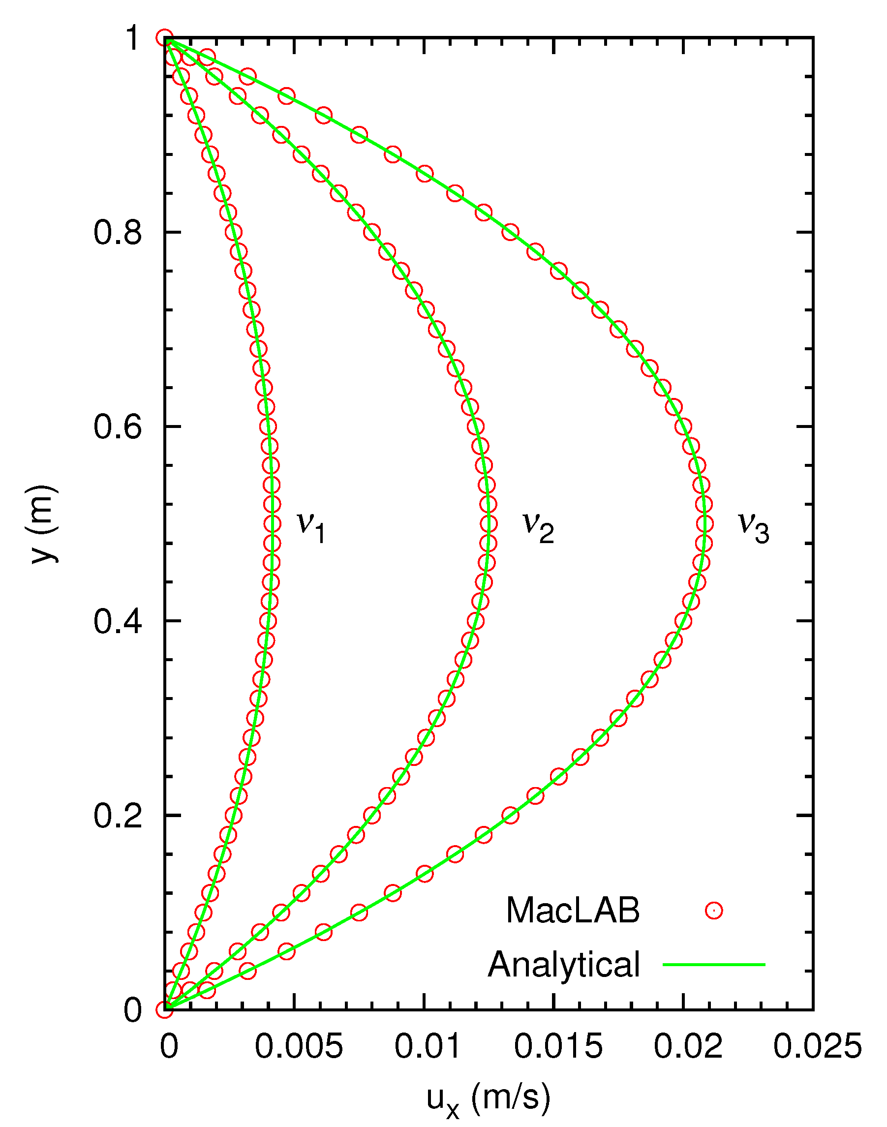
Figure 3.
2D cavity flow within a square for . The top lid moves at a velocity of and , and the other three sides are fixed, or no slip boundary condition is applied. After the steady solution is obtained, the flow pattern in velocity vectors shows a primary vortex and two secondary vortices.
Figure 3.
2D cavity flow within a square for . The top lid moves at a velocity of and , and the other three sides are fixed, or no slip boundary condition is applied. After the steady solution is obtained, the flow pattern in velocity vectors shows a primary vortex and two secondary vortices.

Figure 4.
2D cavity flow within a square for . The top lid moves at a velocity of and , and the other three sides are fixed, or no slip boundary condition is applied. After the steady solution is obtained, the comparison of the velocity profile along the y direction through the geometric centre of the cavity with the numerical solution by Ghia et al. [32], showing good agreement.

Figure 5.
2D cavity flow within a square for . The top lid moves at velocity of and , and the other three sides are fixed, or no slip boundary condition is applied. After the steady solution is obtained, the comparison of the velocity profile along the x direction through the geometric centre of the cavity with the numerical solution by Ghia et al. [32], showing good agreement.

Figure 6.
Taylor–Green vortex within the domain for . The initial conditions are and with . The periodic boundary conditions are used. Shown here is the flow pattern in velocity vectors at s, the same vortex pattern remaining as that at the initial state.
Figure 6.
Taylor–Green vortex within the domain for . The initial conditions are and with . The periodic boundary conditions are used. Shown here is the flow pattern in velocity vectors at s, the same vortex pattern remaining as that at the initial state.

Figure 7.
Taylor–Green vortex within the domain for . The initial conditions are and with . The periodic boundary conditions are used. Shown here is the comparisons of the relative velocity profiles for at and at , matching the analytical solutions of and at s.
Figure 7.
Taylor–Green vortex within the domain for . The initial conditions are and with . The periodic boundary conditions are used. Shown here is the comparisons of the relative velocity profiles for at and at , matching the analytical solutions of and at s.

Figure 8.
3D cavity flow within a cube for . The top lid moves at a velocity of , and , and the other five sides are fixed, or no slip boundary condition is applied. After the steady solution is reached, the flow pattern in vectors in the centroidal plane show the primary and secondary vortices.
Figure 8.
3D cavity flow within a cube for . The top lid moves at a velocity of , and , and the other five sides are fixed, or no slip boundary condition is applied. After the steady solution is reached, the flow pattern in vectors in the centroidal plane show the primary and secondary vortices.

Figure 9.
3D cavity flow within a cube for . The top lid moves at a velocity of , and , and the other five sides are fixed, or no slip boundary condition is applied. After the steady solution is reached, the flow pattern in vectors in the centroidal plane shows one pair of strong secondary vortices at the bottom and one pair of weak secondary vortices at the top.

Figure 10.
3D cavity flow within a cube for . The top lid moves at a velocity of , and , and the other five sides are fixed, or no slip boundary condition is applied. After the steady solution is reached, the flow pattern in vectors in the centroidal plane shows a pair of third vortices close to the inflow boundary.

Figure 11.
3D cavity flow within a cube for . The top lid moves at a velocity of , and , and the other five sides are fixed, or no slip boundary condition is applied. After the steady solution is reached, the comparisons of the distribution of the velocity component on the vertical plane centerline with the results by Wong and Baker [33] and Jiang et al. [34].

Publisher’s Note: MDPI stays neutral with regard to jurisdictional claims in published maps and institutional affiliations. |
© 2020 by the author. Licensee MDPI, Basel, Switzerland. This article is an open access article distributed under the terms and conditions of the Creative Commons Attribution (CC BY) license (http://creativecommons.org/licenses/by/4.0/).
Share and Cite
MDPI and ACS Style
Zhou, J.G. Macroscopic Lattice Boltzmann Method. Water 2021, 13, 61. https://doi.org/10.3390/w13010061
AMA Style
Zhou JG. Macroscopic Lattice Boltzmann Method. Water. 2021; 13(1):61. https://doi.org/10.3390/w13010061
Chicago/Turabian StyleZhou, Jian Guo. 2021. "Macroscopic Lattice Boltzmann Method" Water 13, no. 1: 61. https://doi.org/10.3390/w13010061
Note that from the first issue of 2016, this journal uses article numbers instead of page numbers. See further details here.