The employment of exploratory statistics aimed to estimate the degree of variability assuming that the variables studied are affected by the pluviometric index. Thus, the discussion in the present paper is distributed in topics to each biweekly analyzed chemical component in groundwater.
3.1. Spatiotemporal Distribution and Exploratory Statistic of Cadmium in Groundwater
From the data obtained in the analysis of Cd
2+ concentration, a basic descriptive statistic was performed (minimum, maximum, mean, standard deviation and median values) to understand the relation between the main parameters and the sampled wells in the research field. The values of mean monthly cadmium flow, among all wells, variated from 1.48 to 44 µg L
−1.
Table 2 presents the mean monthly values and their respective standard deviations of the obtained concentrations in the samples, as well as the values of minimum, maximum, mean, standard deviation and median in each well during the period studied.
The influence of the spatiotemporal behavior of the aquifer hydraulic charge on the mean monthly cadmium concentration was correlated to the parameter of mean monthly pluviometric level of the study region as if it was the recharge level or water volume level of the aquifer [
23]. A
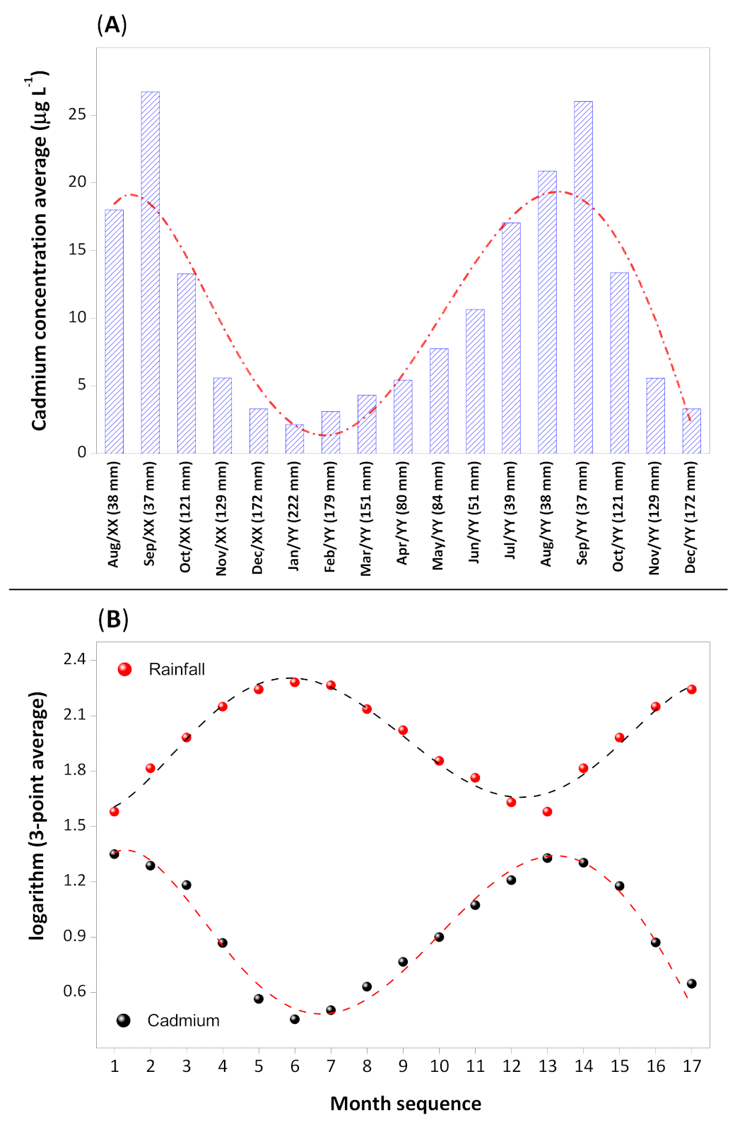
Figure 3A shows a seasonable or cyclic behavior of the increasing and decreasing in the mean monthly flow of the mentioned metallic cation throughout time. With a statistical technique to aid the data interpretation, a trend curve was elaborated (short-dash-dot curve of
Figure 3A) for the cadmium concentration in the aquifer in a temporal function in which the analysis occurred.
Through the model, we can observe that the cadmium concentration exhibits a crescent tendency in the dry season (April through September) and a decrescent tendency in the rainy season (October through March). The transformation of the concentration data and pluviometric index to the logarithmic base (see
Figure 3B) demonstrates correlative and significative cycles in both parameters analyzed in temporal sampling function. The model indicates that the phenomenon has a periodicity, or it obeys a periodical function, where the mean logarithmic concentration of cadmium is inversely proportional to the magnitude of the monthly seasonable variability of rainfall. The cyclic variation in the cadmium mean monthly flow is indicative that the chemical element does not come from an external source and it is found in the aquifer’s area itself. During the rainy season, there is a dilution effect due to the increase in the aquifer’s water volume. Meanwhile, during the dry season, the low water level in the aquifer causes the opposite process, when the cadmium concentration increases.
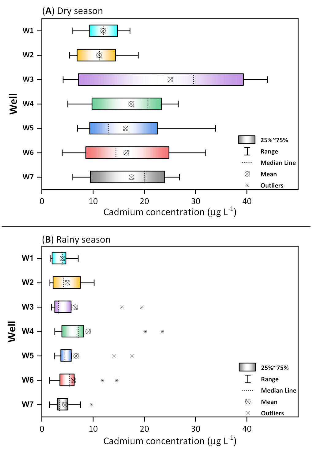
Figure 4 presents a boxplot diagram [
24] that provides a better representation of the observed data variation in each well for the cadmium concentration during the dry (
Figure 4A) and rainy seasons (
Figure 4B). The distinction between the rainy and dry seasons is very clear as it is shown in both boxplot diagrams. A general seasonal distinction is based on the only components from the hydric balance on a monthly scale as shown in
Figure 3B. Analyzing the dataset of each well during the dry season (
Figure 4A), well W3 presents the highest dispersion on the values of cadmium concentration in the interquartile range, which consists in a difference between the third and the first quartile. One of the concentration variability factors is the process of groundwater pumping during the driest seasons, influenced by the extremely low levels of the groundwater, resonating significantly in the chemical compound’s concentration in the aquifer [
16]. Comparatively, the lowest dispersion in the interquartile range for the values of cadmium concentration was observed in the well W1. A factor for the lowest dispersion in the concentration of cadmium may be related to the location of the well W1 that is situated in a green area with a low population density. Analyzing the median lines, the wells W5 and W6 present a positive asymmetric distribution, indicating that the median is close to the first quartile or that the median value is lower than the mean value. Meanwhile, the wells W2, W3, W4 and W7 present a negative asymmetric distribution. It was verified for the well W1 that the mean and median values are coincidental demonstrating a symmetric distribution. It is important to point out that the median is the central tendency measure more appropriate when the data present asymmetric distribution since the arithmetic mean is influenced by the extreme values.
Contrastingly, cadmium concentration is lower in groundwater collected during the rainy season (
Figure 4B) with a mean monthly below 10 μg L
−1. As previously shown in
Figure 3B, this result is due to the dilution of the concentration by groundwater recharge. However, the descriptive parameters in the boxplots present anomalous values (outliers) in almost every well studied (except in wells W1 and W2). The anomalous values are related to the first rainy month (October) in which the cadmium concentrations are still high in comparison to the dataset for the period, implying that the dilution factor is in the initial phase in the aquifer due to the dependence of the groundwater recharge rate [
25].
Table 3 presents mean values for the monthly rainfall index (MRI), pH and cadmium concentration. The monthly mean values of pH were calculated based on the pH measurements of groundwater in each well studied.
To verify the dependence degree of the mean monthly flow to the rainfall index and the pH of the water collected, Pearson correlation coefficient was applied with paired Student’s
t-test with a significance level of 5% on the correlation coefficient obtained, where H
0: r = 0 and H
1: r ≠ 0. As shown in
Table 4, there is a moderate relation between the MRI parameters and the mean cadmium concentrations in groundwater.
Comparing the calculated t value (−5.352) to the critical value for the Student’s t-distribution (±2.131), t value is out of the region for the H0 hypothesis to be accepted. Thus, we can conclude that there is enough evidence to correlate the concentration parameters of Cd(II) to MRI. Concerning the mean monthly of Cd(II) and the mean pH, the Pearson coefficient obtained shows that there is a weak relation. Comparing the calculated t value (−0.379) to the critical value for the Student’s t-distribution (±2.131), t value is in the region for the H0 hypothesis to be accepted. Thus, we can conclude that there is not enough evidence suggesting that there is a relation between the cadmium concentration and the pH. The statistical result obtained through Pearson’s correlation indicates that the variability in groundwater pH is not caused by the variation in cadmium concentration in function of the region’s rainfall index.
3.2. Spatiotemporal Distribution and Exploratory Statistic of Lead in Groundwater
Table 5 presents the mean monthly values and their respective standard deviations of the obtained samples concentrations, as well as minimum, maximum, mean, standard deviation and median values in each well for study period.
The mean monthly lead flow variation (minimum = 1.39 µg L
−1 and maximum = 44.9 µg L
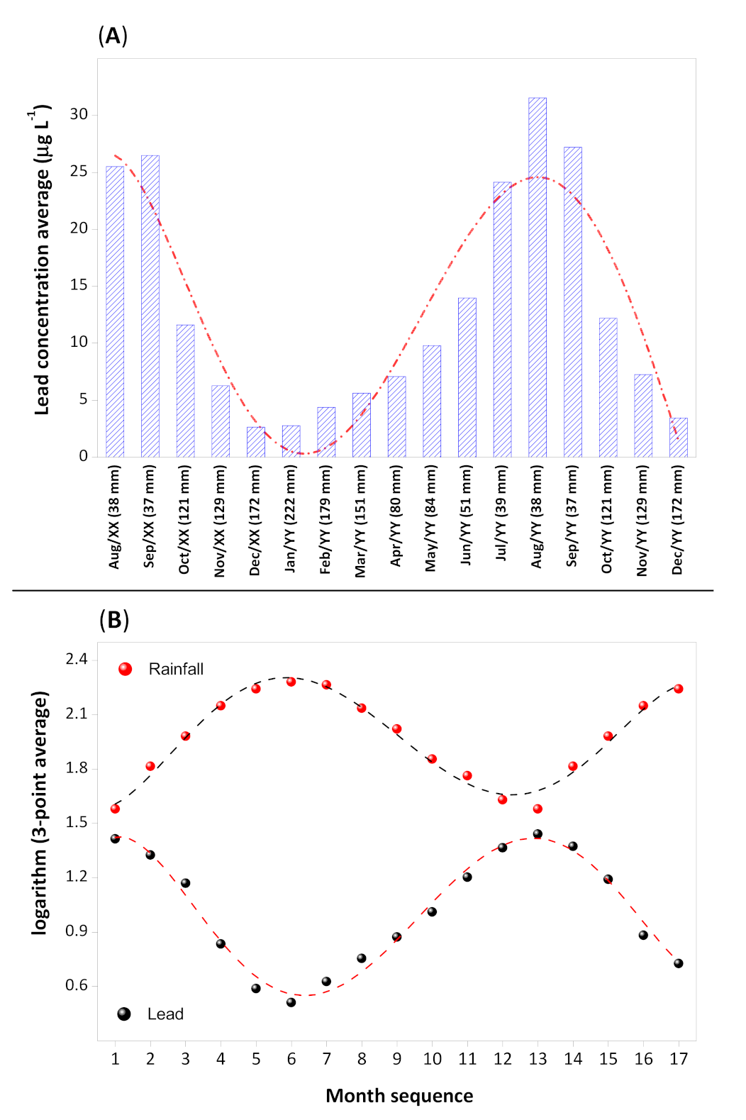
−1) in the wells was similar to what was observed for the cadmium concentrations. The concentration magnitude varied with the monthly period of the sampling and the geographical position of the wells studied. With the obtained data of lead concentrations, a spatiotemporal graph for the variation in total mean lead concentration was plotted in the logarithmic base (
Figure 5B).
The profile of lead concentration variation in groundwater followed a periodicity model in function of time and the highest concentration magnitudes were observed during the dry season. Analyzing comparatively the lead spatiotemporal behavior, we can conclude that this element is found in the aquifer itself. Its dilution in the groundwater is due to increasing in hydric volume and consequently to the recharge flow (pluviometric level). For better visualization of what was verified before,
Table 6 presents the lead mean concentration in wells W1 to W7 with their respective standard deviations, in the rainy season (October through March) and in the dry season (April through September). Evaluating the boxplot diagram, the highest dispersions and lead concentration distributions were observed during the dry season (
Figure 6A). As observed before, well W1 presented the lowest variability of concentration in the sampling temporal scale. In general, the medians are very close to the concentration means, indicating that the observed concentrations in the dry season are a symmetrical normal distribution. For the rainy season, the mean monthly lead flow values (
Figure 6B) were below 10 μg L
−1. However, outlier concentrations were observed in wells W5, W6 and W7 and these outlier values correspond precisely to the beginning of the rainy season.
In the Pearson test to analyze the dependence degree of Pb2+ concentration to the mean pH of the collected water, with a correlation coefficient (ρ) of −0.0066, there is an indication that these two variables are not correlated. To confirm that the variability in lead concentration is not influenced by the pH or vice versa, a two-tailed Student’s t-test with a significance level of 5% was applied and considering the null and true hypothesis as r = 0 and r ≠ 0, respectively. Comparing the calculated t value (−0.26) to the critical value for the Student’s t-distribution (±2.131), the calculated t value is in the region for the H0 hypothesis to be accepted. Thus, we can conclude that there is not enough evidence to support that Pb2+ concentration and pH are correlated.
3.3. Spatio-Temporal Distribution and Exploratory Statistic of Copper in Groundwater
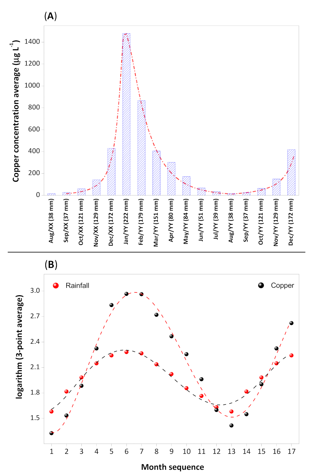
In the copper concentration spatiotemporal distribution study, it was identified an inverted behavior when compared to the cadmium and lead in groundwater. The mean monthly copper flow values, among all wells, variated from 4.8 to 2.479 µg L
−1 (see
Table 7). In addition, the standard deviation values are higher than the mean, indicating that the copper concentrations are distributed around a wide range of values throughout the entire period.
The copper mean monthly concentration through time and its relation of its logarithmic base to the pluviometric index are represented in
Figure 7A,B, respectively. Analyzing
Figure 7A, it can be observed that the copper concentration in the aquifer increases significantly during the month with higher rainfall intensity. After its concentration peak, the reduction of copper presence in groundwater is gradual and concomitantly with the pluviometric index. Its residence time or memory effect in the aquifer is around 5 months approximately. Through
Figure 7B it is possible to observe that the copper concentration in groundwater is directly proportional to the pluviometric level. This behavior indicates strongly that the greater source of copper in groundwater is originated out of the aquifer. It is known that the recharge time can be around days to years depending directly on the hydrogeology properties of the aquifer and of the levels of direct recharge areas. Through the copper variability characterization in groundwater (see
Figure 7B), the present study points out that the response of the aquifer’s recharge in function of rainfall regime is between 1–2 months, given that the magnitude of the maximum copper concentration is reached after the first period of rainfall. This result corroborates studies of the water table monitoring facing correlations to the pluviometric level in the region [
26].
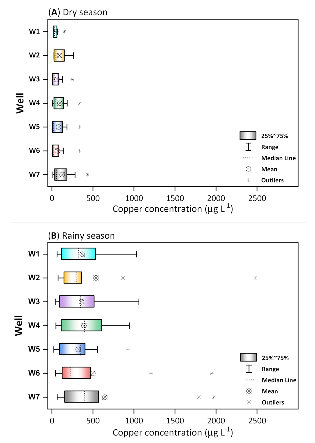
Applying the boxplot diagram (
Figure 8) to the copper concentration variability for both pluviometric periods, it is observed more clearly the pluviometric influence when the higher copper concentrations happen during the rainy season (October through March) and its reduction during the dry season (April through September). Differently from the data obtained for cadmium and lead during the dry season, all wells presented outliers concentrations, which contributed to a higher asymmetric distribution of the data (
Figure 8A). This adverse characteristic is related to the beginning of the dry season (April, May and June) when the copper concentration is still relatively high in the aquifer. Through
Figure 8B that represents the rainy season, the concentrations magnitudes are about 5 times higher in comparison to the dry season mean. From this observation, it is presented in the item “Conclusion” an analysis of the possible causes of the increase in its concentration during the rainy season. Analyzing the dataset, wells W2, W5, W6 and W7 are the ones that present the higher concentration variability during the rainy season. With the mean monthly pluviometric index values, pH and Cu
2+ concentration, it was verified the dependence degree of these parameters through Pearson’s test. As shown in
Table 8, there is a strong correlation between the parameters MRI and copper mean concentrations in groundwater. This conclusion is confirmed through Student’s
t-test with a significance level of 5%, where H
0: r = 0 and H
1: r ≠ 0. Comparing the calculated
t value (8.743) to the critical value for the Student’s t-distribution (±2.131), the calculated
t value is out of the region for the H
0 hypothesis to be accepted. Thus, we can conclude that there is enough evidence that the parameters of Cu
2+ concentration and mean monthly pluviometric index are correlated.
As for the relation between Cu2+ concentration and the groundwater pH, the Pearson coefficient value obtained shows that there is a moderated correlation. This conclusion is confirmed by the obtained t value (3.486) being higher than the critical value for the Student’s t-distribution (±2.131), indicating that the calculated t value is out of the region for the H0 hypothesis to be accepted. Thus, we can conclude that the pH of the aquifer is influenced by the presence and concentration of Cu2+.
3.4. Principal Component Analysis
A Principal Component Analysis (PCA) was employed to determine the discriminant functions in order to confirm the spatiotemporal variations of chemical elements in groundwater.
Table 9 presents two principal components (PC) that obtained the most significant percentage of variability (totalizing 98.3% of the data variability) and the vectors’ values per parameter.
The criterion employed in this kind of analysis was the evaluation of the weight of the variable associated with a component. Weights above 0.7 are indicative of strong association; for values between 0.5–0.7, the variable is considered to be moderately associated; weights inferior to 0.5, the variable has a weak association to the component [
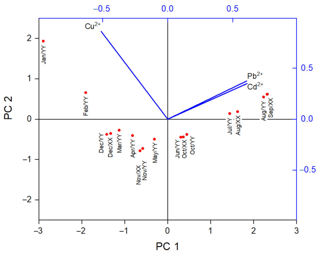
27]. The first component (82.2%) is associated with a positive moderate variance for cadmium and lead during the dry season. In the same component, the copper variability presented a negative and moderate association for the same period. The second component (16.1%) was strongly associated solely with copper, which can be interpreted as the influence of the rainy season. According to a visual interpretation of the bidimensional representation of the two first principal components (
Figure 9), the influence vectors are identified into two groups, as evidenced previously in the exploratory statistics analysis. The variable of copper concentration was close to CP2 axis, showing that the months of January and February (months of the highest pluviometric levels) present high correlations.
Contrastingly, cadmium and lead are more representatives to the CP1 axis, where we can observe that the vectors are equivalent and that the concentrations of these elements are correlative to the months of lowest pluviometric index (July through September). The acute angle of the vectors’ points to a high correlation between the two variables.


