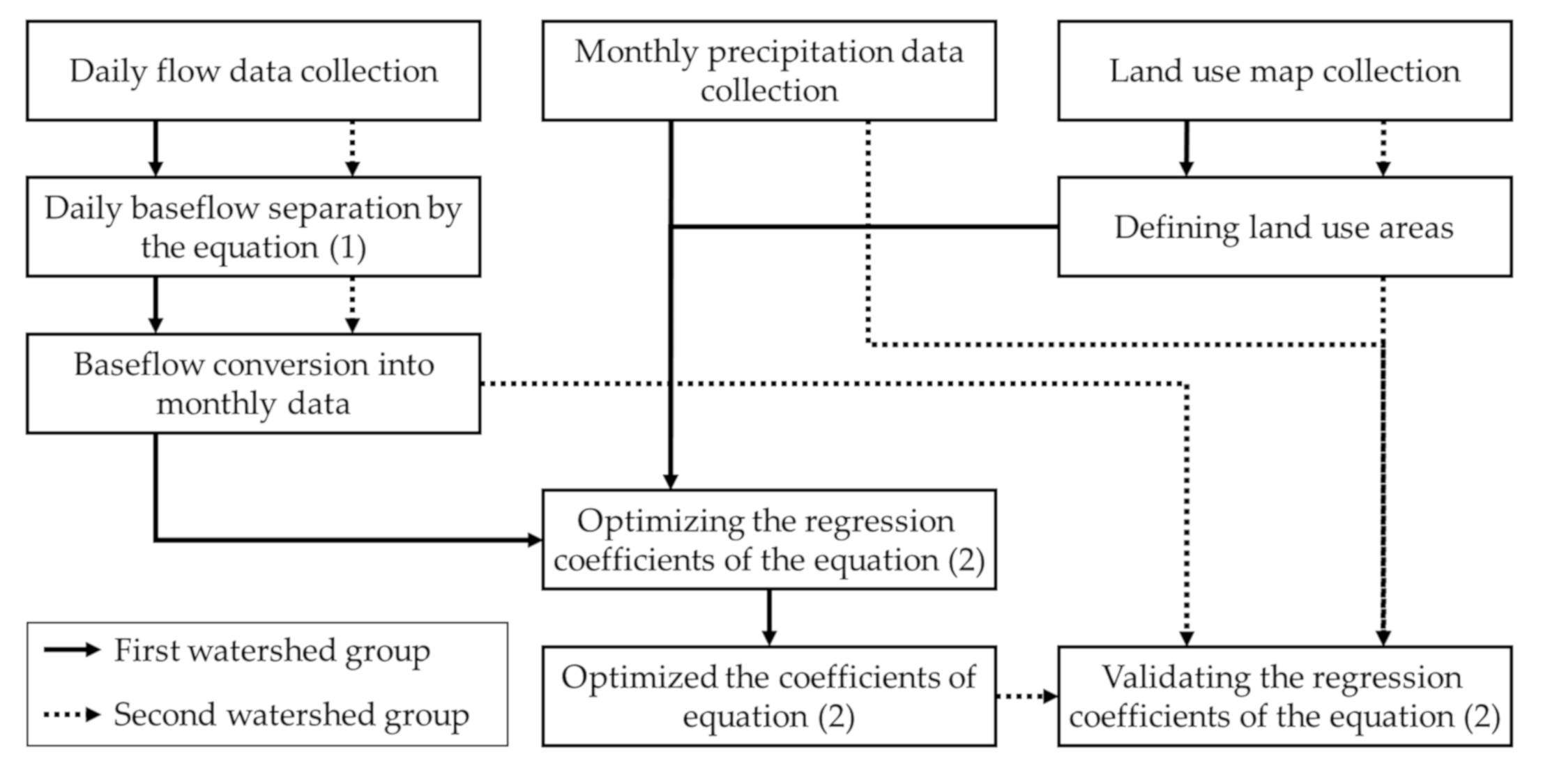
3.1. Determination of Regression Model Coefficients
Optimal values for the seven coefficients in Equation (2) for predicting the monthly baseflow were determined by GA based on the monthly baseflow estimated for each watershed and the monthly flow that was distinguished using the Eckhardt filter equation (Equation (1)). The coefficients for which the smallest difference between the monthly baseflow separated using Equation (1) and the monthly baseflow estimated using Equation (2) was observed in each watershed were determined to be optimal. In this study, it was deemed necessary to measure the separated monthly baseflows and to develop the criteria for examining the validity of the estimated monthly baseflow. Duda et al. [
32] reported that the estimated result is applicable when the R
2 is higher than 0.65 and the difference is 45% or less. Skaggs et al. [
33] mentioned that the result is applicable when the Nash–Sutcliffe efficiency (NSE) is higher than 0.50, and Wang et al. [
34] suggested that it is applicable when the NSE is higher than 0.50, the R
2 is higher than 0.60, and the PBIAS is ±15%. Moriasi et al. [
35] deemed the result to be applicable when the R
2 is higher than 0.60, NSE is higher than 0.50, and the PBIAS is less than 15%. In other words, there are various criteria for determining the applicability of the estimated result. The different criteria were summarized in this study, and the applicability of the monthly baseflow was estimated using a scatter plot with an NSE higher than 0.50 and an R
2 higher than 0.60.
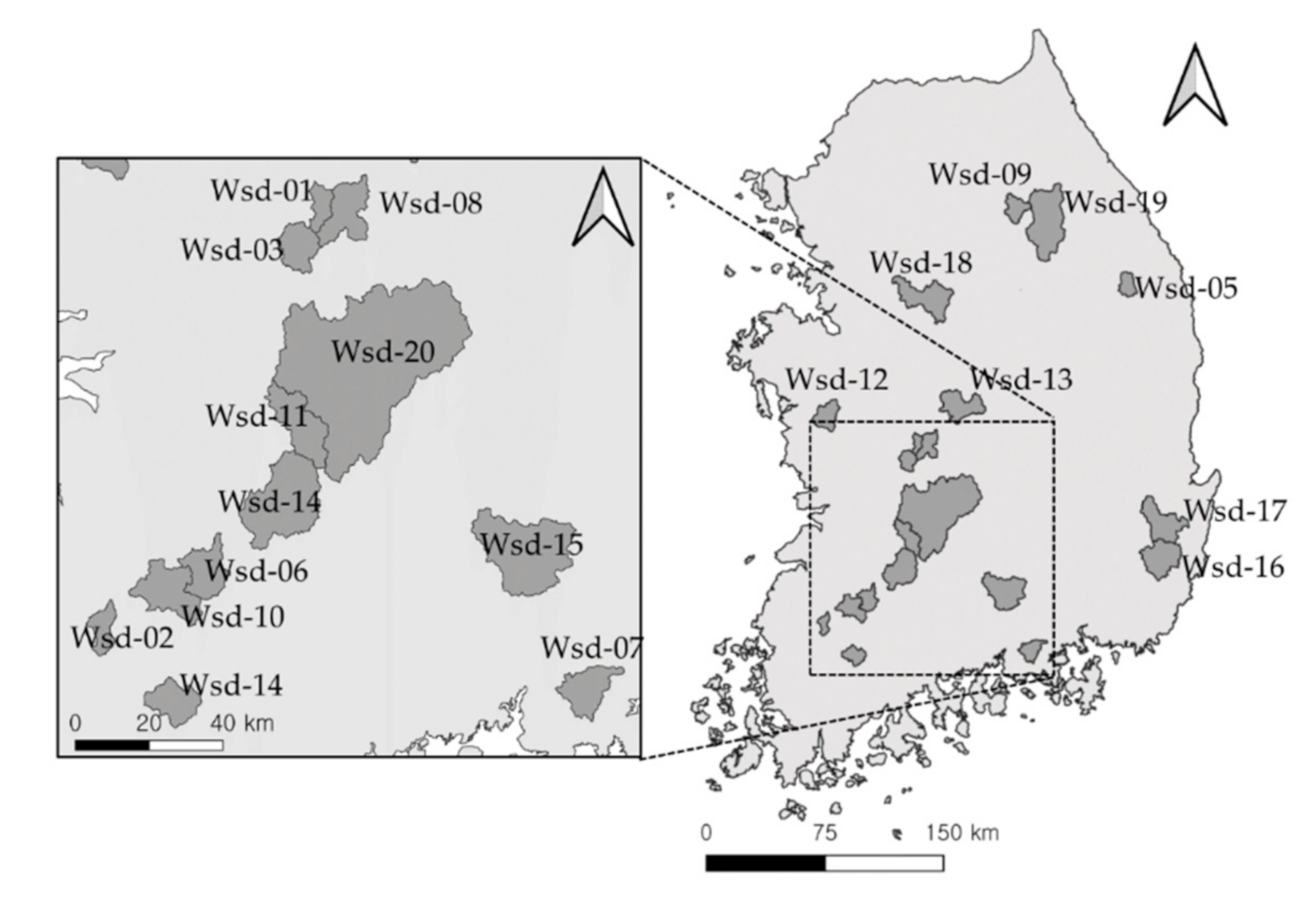
In terms of the optimized coefficients for the 11 watersheds in the first group,
CURBN ranged from 0.00289 (Wsd-04) to 0.06314 (Wsd-04),
CAGRL from 0.10076 (Wsd-01) to 0.49061 (Wsd-06),
CFRST from 0.01256 (Wsd-02) to 0.28413 (Wsd-10),
CPAST from 0.0.07913 (Wsd-06) to 0.31460 (Wsd-20),
CWTLD from 0.05222 (Wsd-02) to 0.78599 (Wsd-16),
CBARE from 0.03488 (Wsd-04) to 0.23603 (Wsd-16), and
CWATR from 0.04919 (Wsd-04) to 0.38384 (Wsd-16) (
Table 4). The optimized coefficients in each watershed were obtained when the difference between the separated and estimated baseflows describing baseflow was minimal. Since the purpose of this study is to propose a method for predicting the monthly baseflow in multiple watersheds rather than judging the accuracy of the monthly baseflow prediction for a specific watershed, the final values of the coefficients of Equation (2) were determined based on the average of each coefficient. The coefficients were, therefore, determined to be 0.04 for
CURBN, 0.40 for
CAGRL, 0.20 for
CFRST, 0.18 for
CPAST, 0.48 for
CWTLD, 0.15 for
CBARE, and 0.22 for
CWATR.
In general, the contribution of land use to the baseflow can be considered to be related to the impervious surface ratio. The contribution of urban areas to the baseflow will be low because the impervious surface ratio is high. A CURBN of 0.04 was finally determined for urban areas based on the optimized results; this reflects the conditions of impermeability, as this coefficient is relatively lower than those obtained for other land uses. In contrast, the contribution of wetlands and reservoirs to the baseflow is high because of the constant infiltration of water. The value of 0.48 for CWTLD also appears to reflect this condition, as it is relatively high as compared to the coefficients for other types of land use.
It is noteworthy that the coefficient for agricultural land, CAGRL, had the second highest value after CWTLD. Agriculture in Korea is dominated by rice paddies, which are maintained in pond conditions during the rice cultivation period from May to October, resulting in a similar contribution to the baseflow as wetland. The contribution of agriculture to the baseflow should, therefore, be similar to that of wetland; this condition is sufficiently reflected in the coefficient for agriculture.
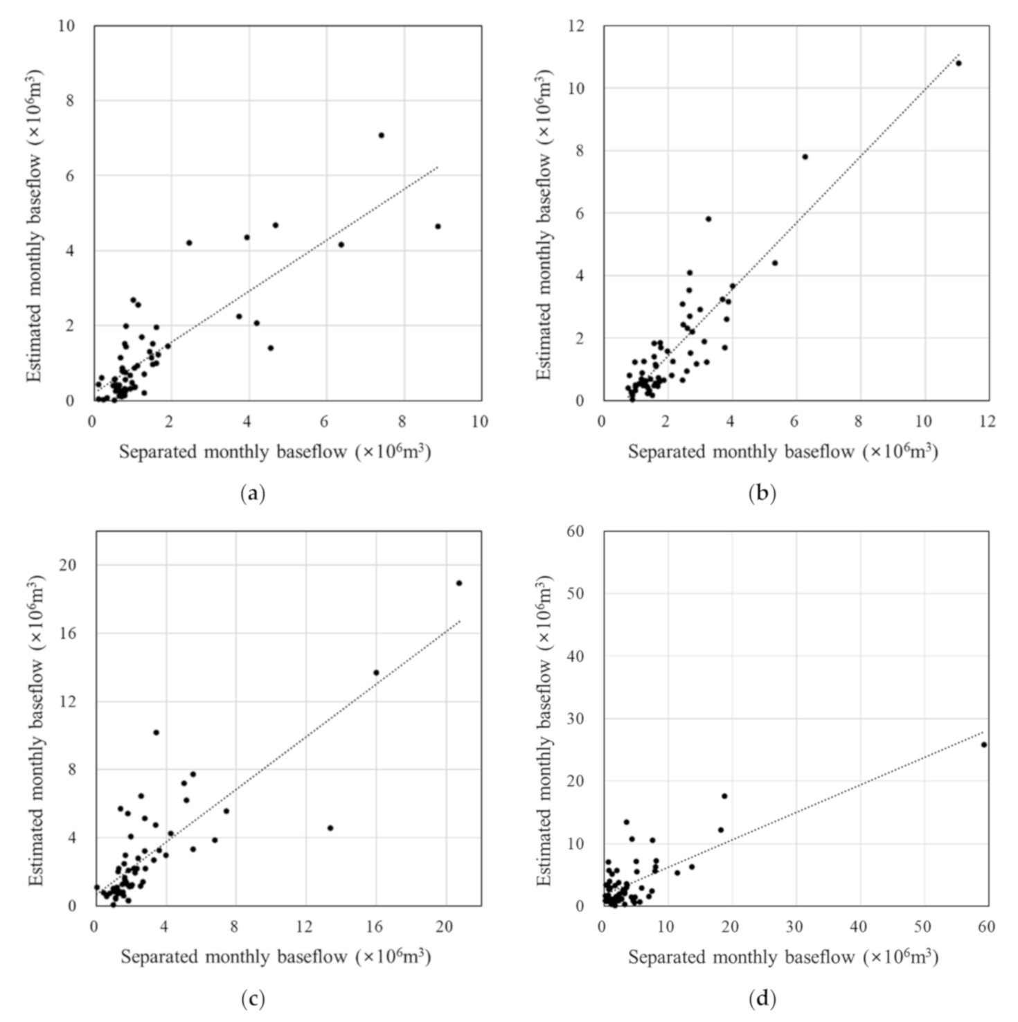
The monthly baseflow in the first watershed group was calculated again using Equation (2) by applying the finally determined coefficients, and the suitability of the monthly baseflow was determined by the values of R
2, NSE, and the scatter plot. Both R
2 and NSE showed applicable ranges with R
2 ranging from 0.600 (Wsd-06) to 0.817 (Wsd-16) and NSE from 0.504 (Wsd-01) to 0.677 (Wsd-18 and Wsd-20) (
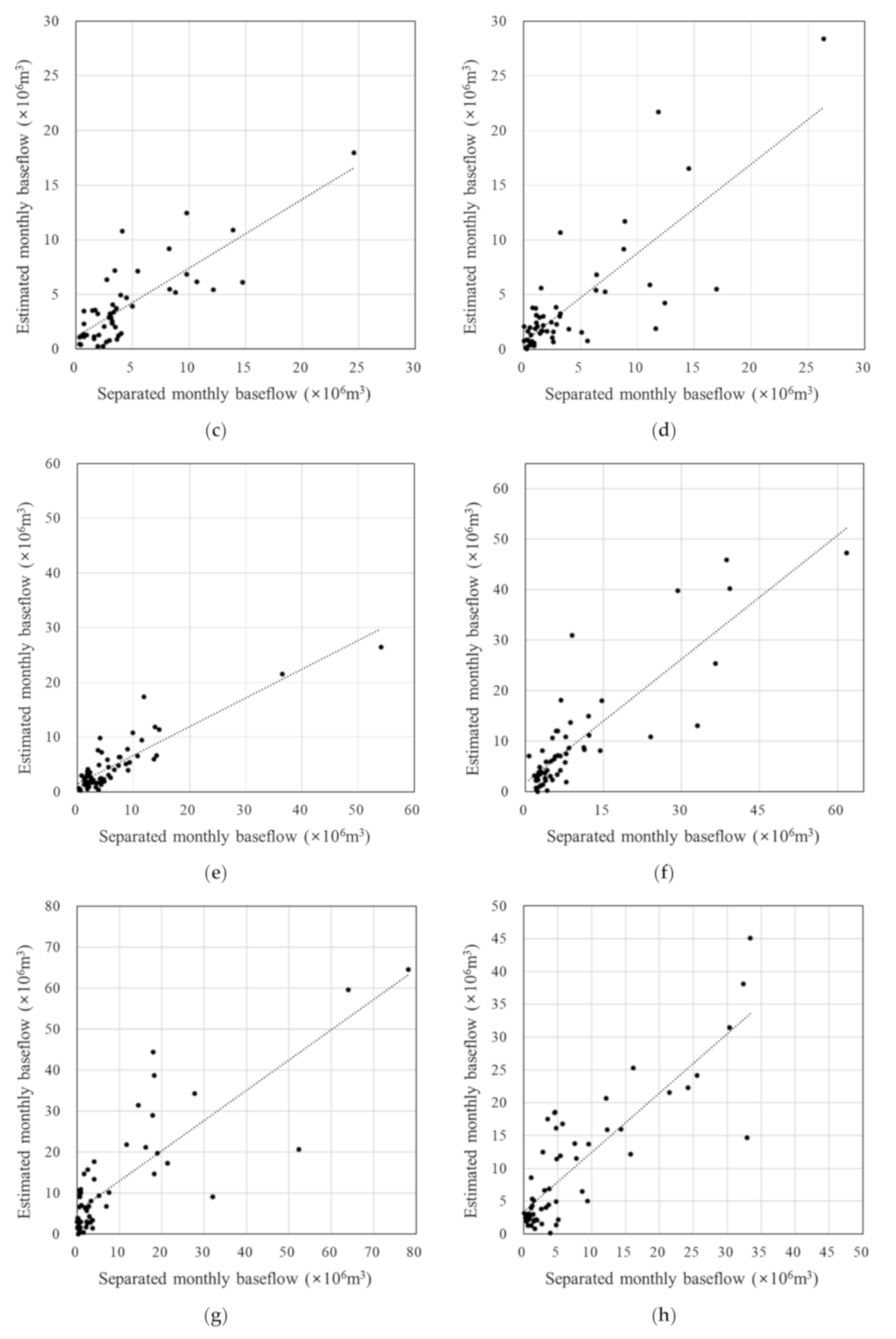
Table 5). Based on the scatter plot, the estimated monthly baseflow tended to be slightly lower than the separated monthly baseflow for Wsd-06, Wsd-08, and Wsd-10; Wsd-20 showed a scattered tendency that was comparable to the other watersheds. Overall, however, there were no significant differences in the tendencies or values obtained via prediction and the separated monthly baseflow (
Figure 3).
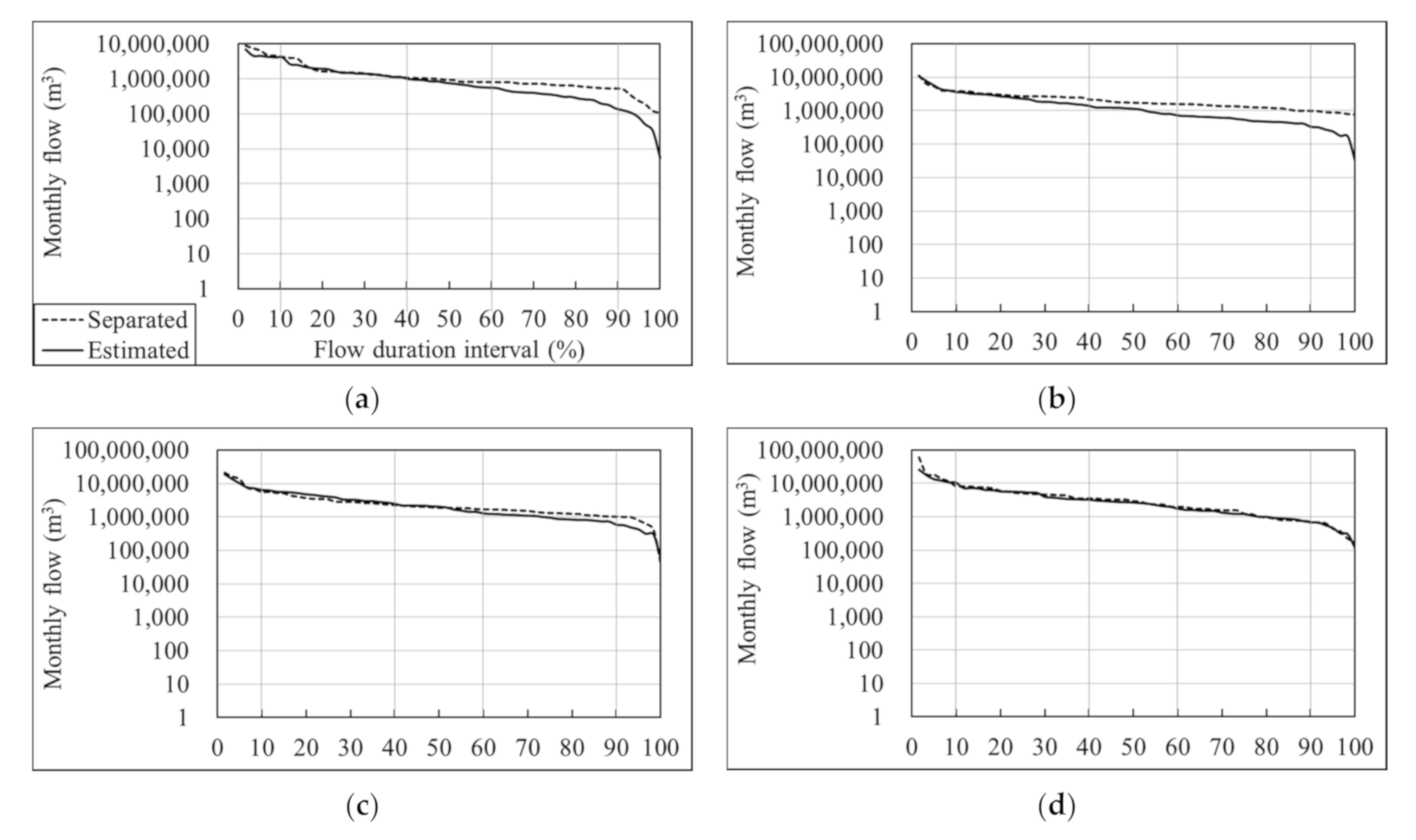
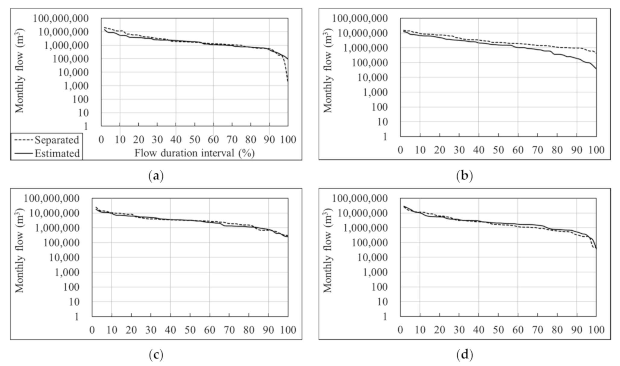
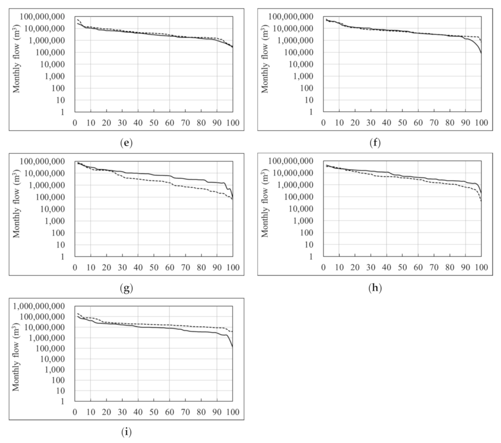
In the plot of flow duration curves, the estimated monthly baseflow did not capture the separated monthly baseflow in the dry-conditions (flow duration intervals from 60% to 90%) and the low-flow (flow duration intervals from 90% to 100%) regimes often; however, it does in the other flow regimes, which are the high-flow (flow duration intervals from 0–10%), the moist-conditions (flow duration intervals from 10% to 40%), and the mid-range flow (flow duration intervals from 40% to 60%) regimes (
Figure 4).
Therefore, the application of optimized coefficients to each watershed will render the estimated monthly baseflow similar to the separated monthly baseflow. Thus, the application of the finally determined coefficients is expected to result in satisfactory predictions.
3.2. Validation of Regression Model Coefficients
When the model parameters that were determined for use for calibration were adjusted for the associated watersheds during calibration, the results derived for these watersheds could be considered satisfactory. However, it is necessary to apply these model parameters to watersheds other than those used in the calibration process to examine whether the model parameters were well calibrated and determine whether the estimated results are applicable. Therefore, in this study, the values determined for the coefficients that correspond to the model parameters in the calibration process were applied to the second group to determine whether the estimated monthly baseflow is also applicable in this group.
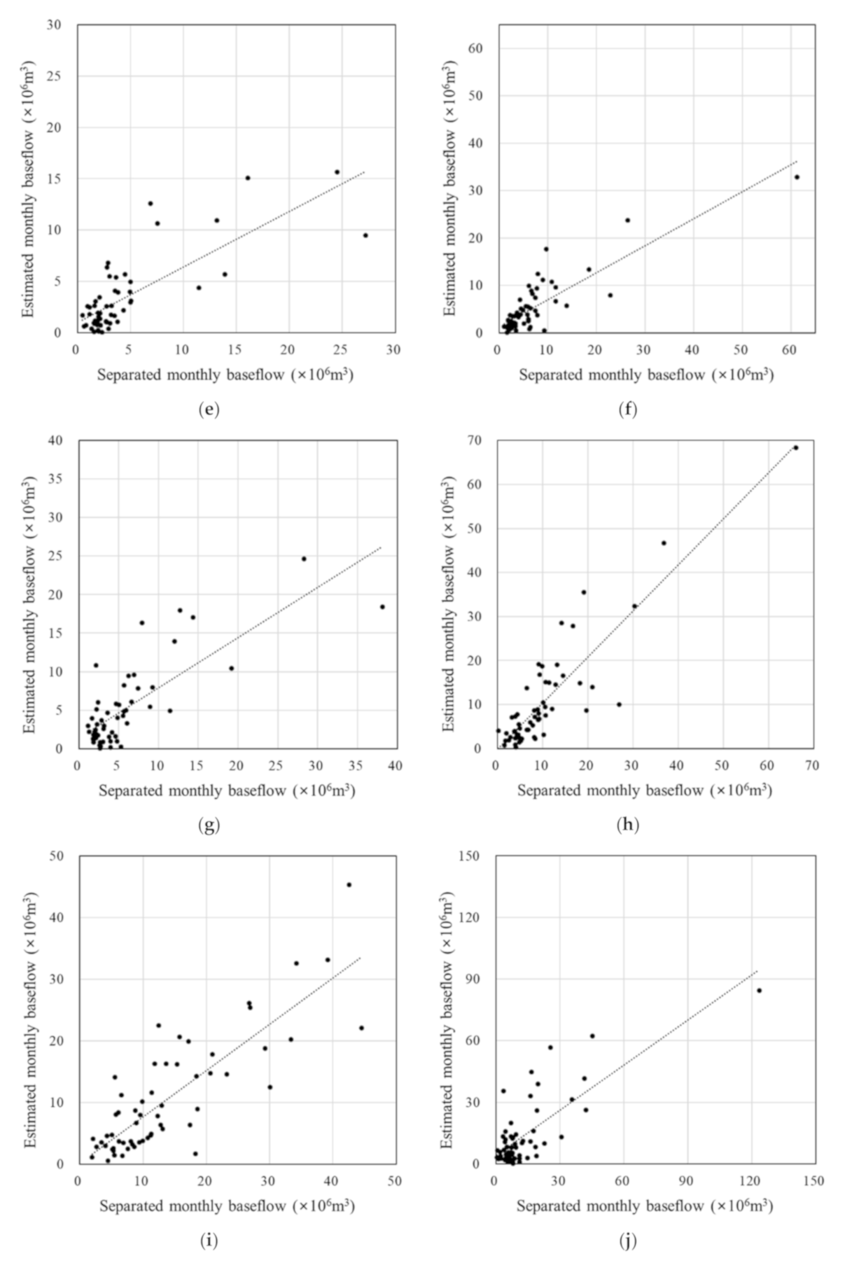
The estimated monthly baseflow was determined to be applicable because the R
2 ranged from 0.618 (Wsd-09) to 0.786 (Wsd-17) and the NSE from 0.567 (Wsd-07) to 0.727 (Wsd-05) (
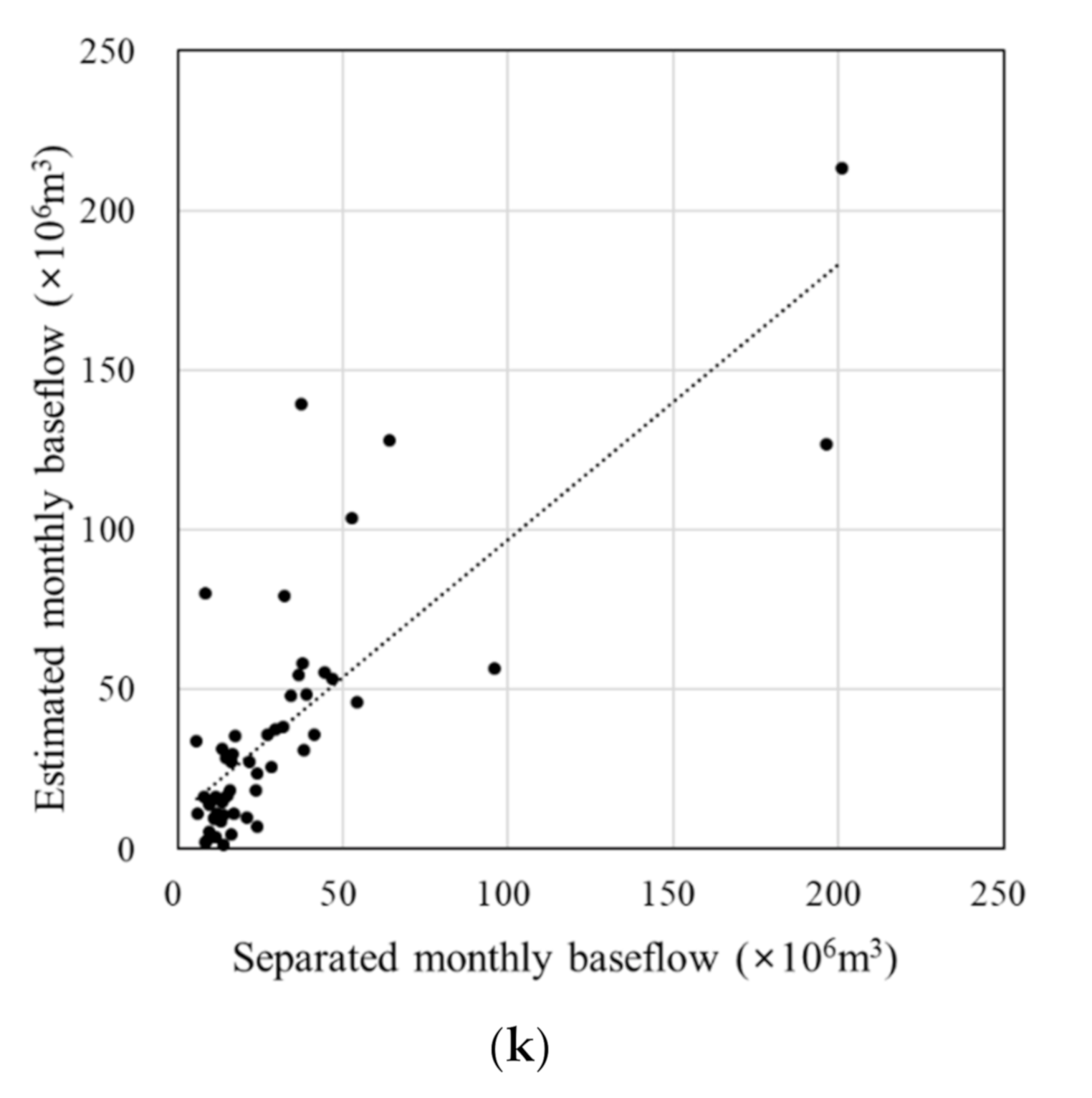
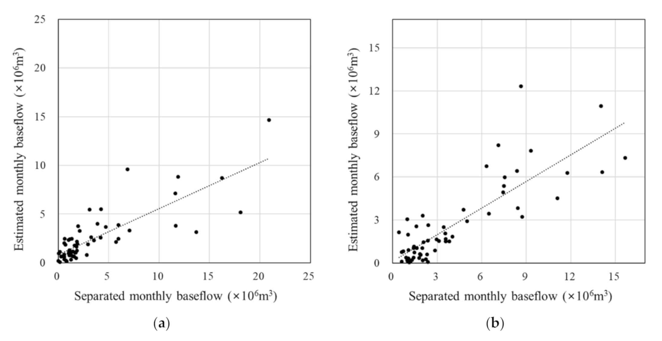
Table 6). Based on the scatter plot, the estimated monthly baseflow tended to be slightly lower than the separated monthly baseflow for Wsd-03, Wsd-11, and Wsd-19. Overall, however, no significant differences were observed in either tendency or value for the estimated and separated monthly baseflow (
Figure 5).
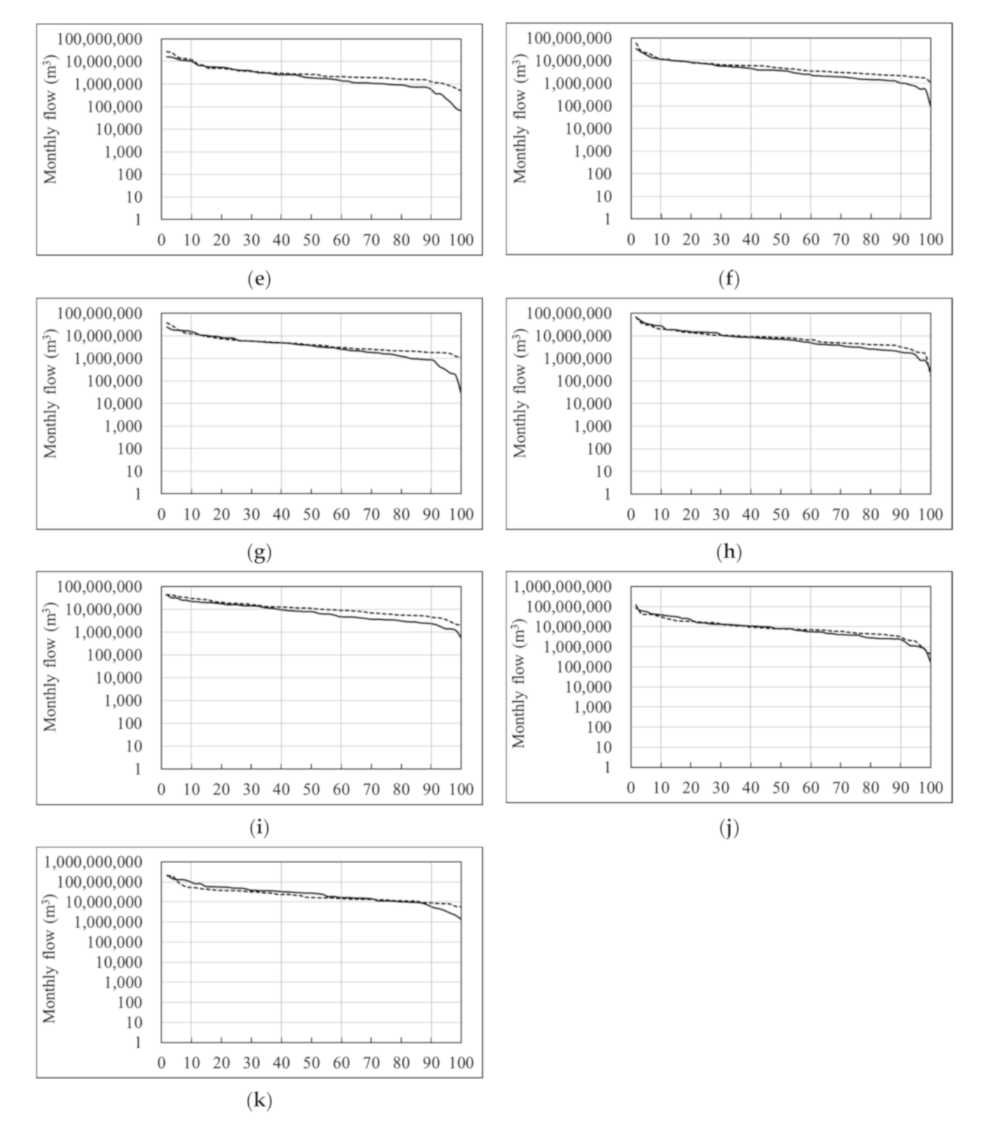
Similar to the results of calibration, the estimated monthly baseflow did not capture the separated monthly baseflow in the dry-conditions and the low-flow regimes often in the flow duration curve plots; however, it does in the other flow regimes, which are the high-flow, the moist-conditions, and the mid-range flow regimes (
Figure 6). Based on flow duration curves in both calibration and validations processes, the estimated monthly baseflow fit to the separated monthly baseflow reasonably in the high-flow and the moist-conditions; however, it did not especially in the low-flow regime. This means that the monthly baseflow approach will be reasonable in the applications with the issues regarding the high flow and the moist conditions such as flooding or nonpoint source pollution analysis. However, caution needs to be exercised when the approach is used for any applications regarding low flow such as water supply simulations in drought.


