
Applying a Graphical Method in Evaluation of Empirical Methods for Estimating Time of Concentration in an Arid Region


Abstract
:1. Introduction
- 1-
- Most of the studies have focused on the analysis of Tc in wet, temperate, and tropic regions. However, the behavior of watersheds in arid regions, despite their significant differences in rainfall pattern, wetness, and vegetation, has been overlooked.
- 2-
- 3-
- The previously mentioned studies applied recorded rainfall-runoff data and evaluated empirical methods at the watershed scale. There is a lack of regional studies evaluating empirical Tc methods
2. Background
3. Materials and Methods
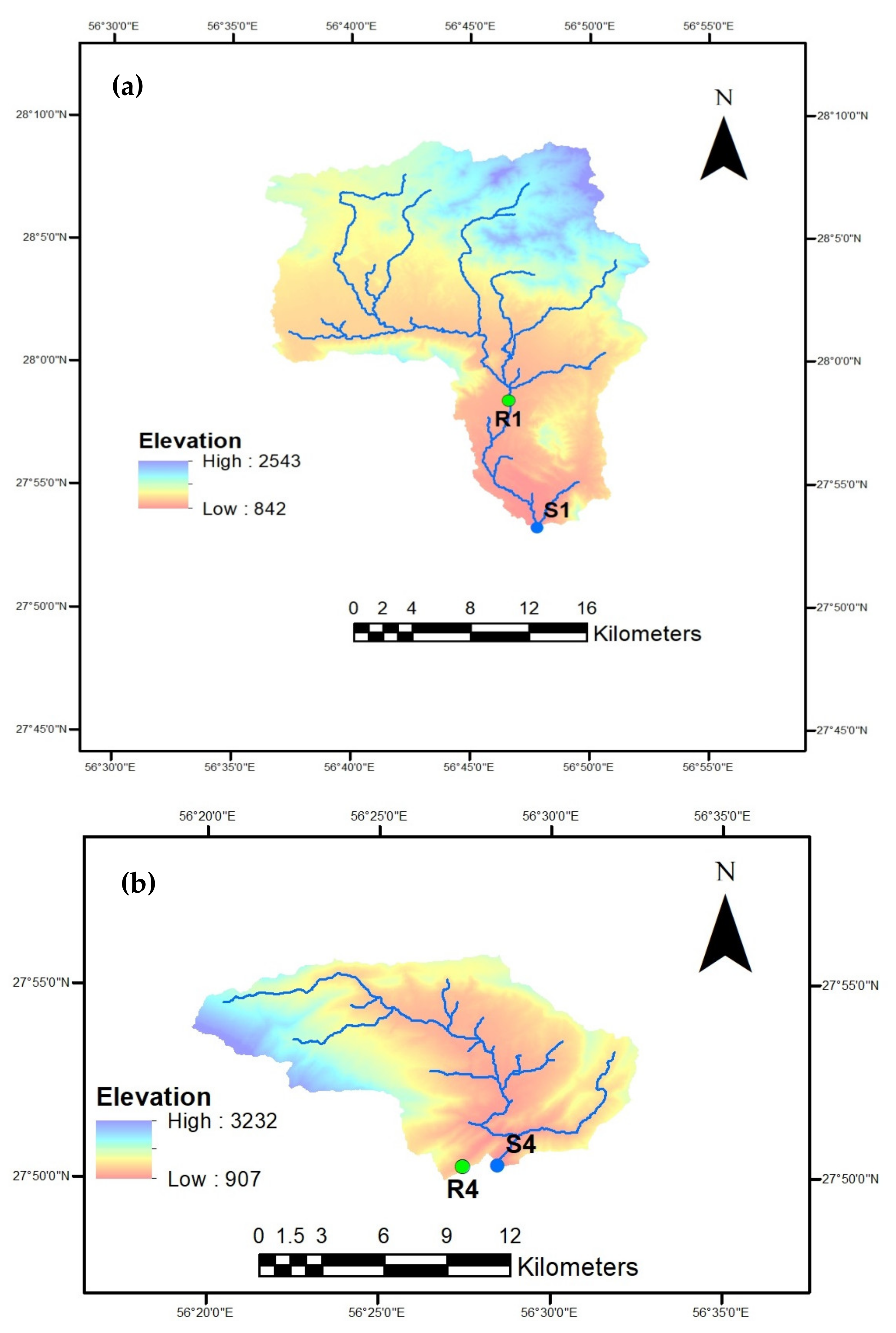
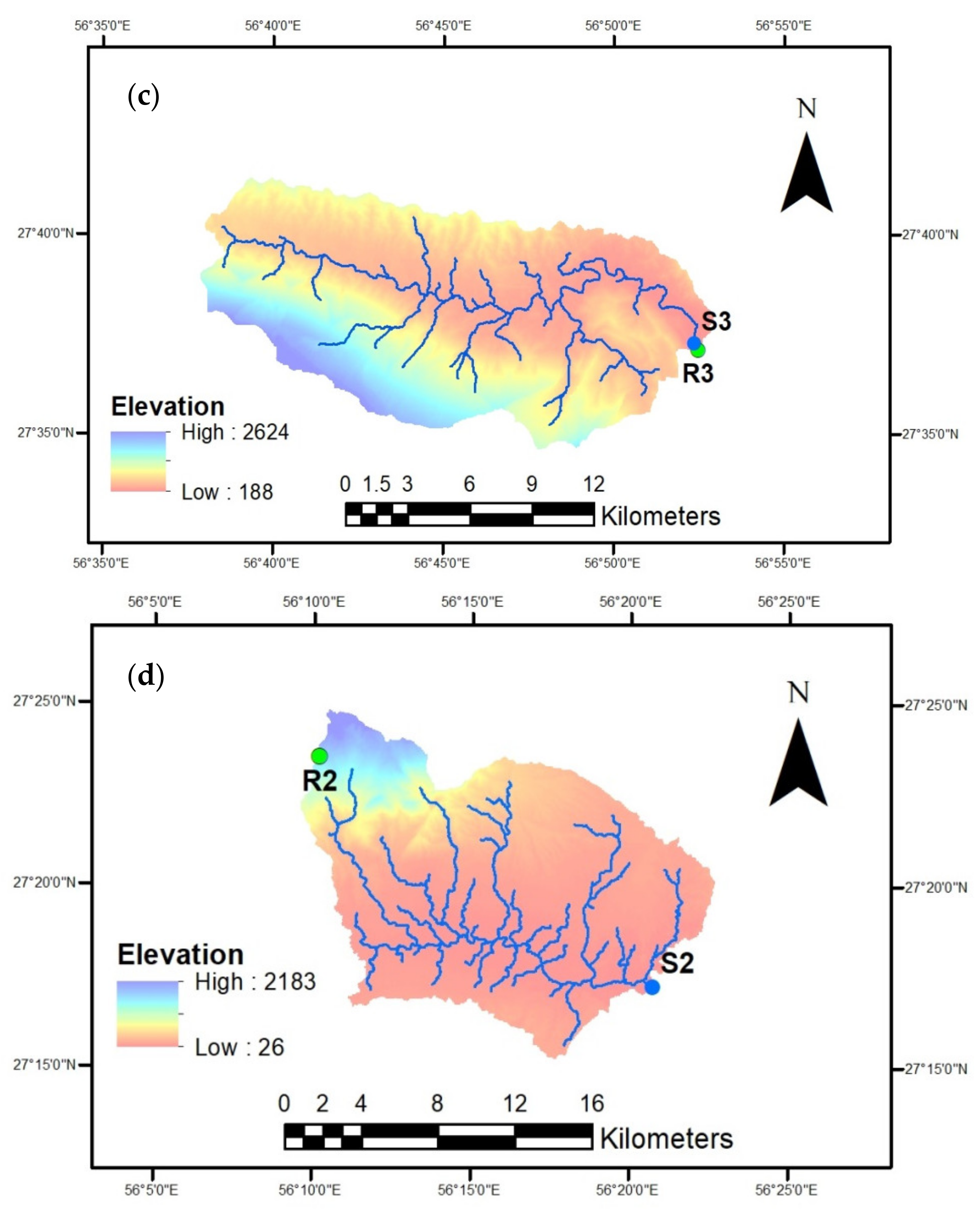
3.1. Study Area

| Sub-Watershed | Shaghrud | Sikhoran | Salubalm | Chahchakur |
|---|---|---|---|---|
| Area (Km2) | 458 | 131 | 200 | 224 |
| Average slope of sub-watershed (%) | 23.6 | 45 | 40.6 | 16 |
| Average elevation (m) | 1354 | 1675 | 848 | 263 |
| Main channel length (Km) | 50 | 24 | 37.5 | 30 |
| Average slope of main channel (%) | 1.2 | 4.4 | 1.1 | 0.8 |
| Perimeter (m) | 154 | 72 | 88 | 99 |
| Compactness coefficient (Cc) | 2.0 | 1.8 | 1.8 | 1.9 |
| Stream length (Km) | 1567 | 594 | 907 | 1243 |
| Drainage density (Km/Km2) | 3.4 | 4.5 | 4.5 | 5.6 |
| Sub-Watershed | Shaghrud | Sikhoran | Salubalm | Chahchakur |
|---|---|---|---|---|
| Average daily rainfall (mm) | 0.44 | 0.68 | 0.79 | 0.47 |
| Maximum daily rainfall (mm) | 75 | 147 | 198 | 155 |
| Minimum daily rainfall (mm) | 0 | 0 | 0 | 0 |
| Coefficient of variation (CV) | 7.4 | 7.7 | 9.2 | 10.9 |
| Annual rainfall (mm) | 159 | 247 | 287 | 172 |
3.2. Empirical Methods
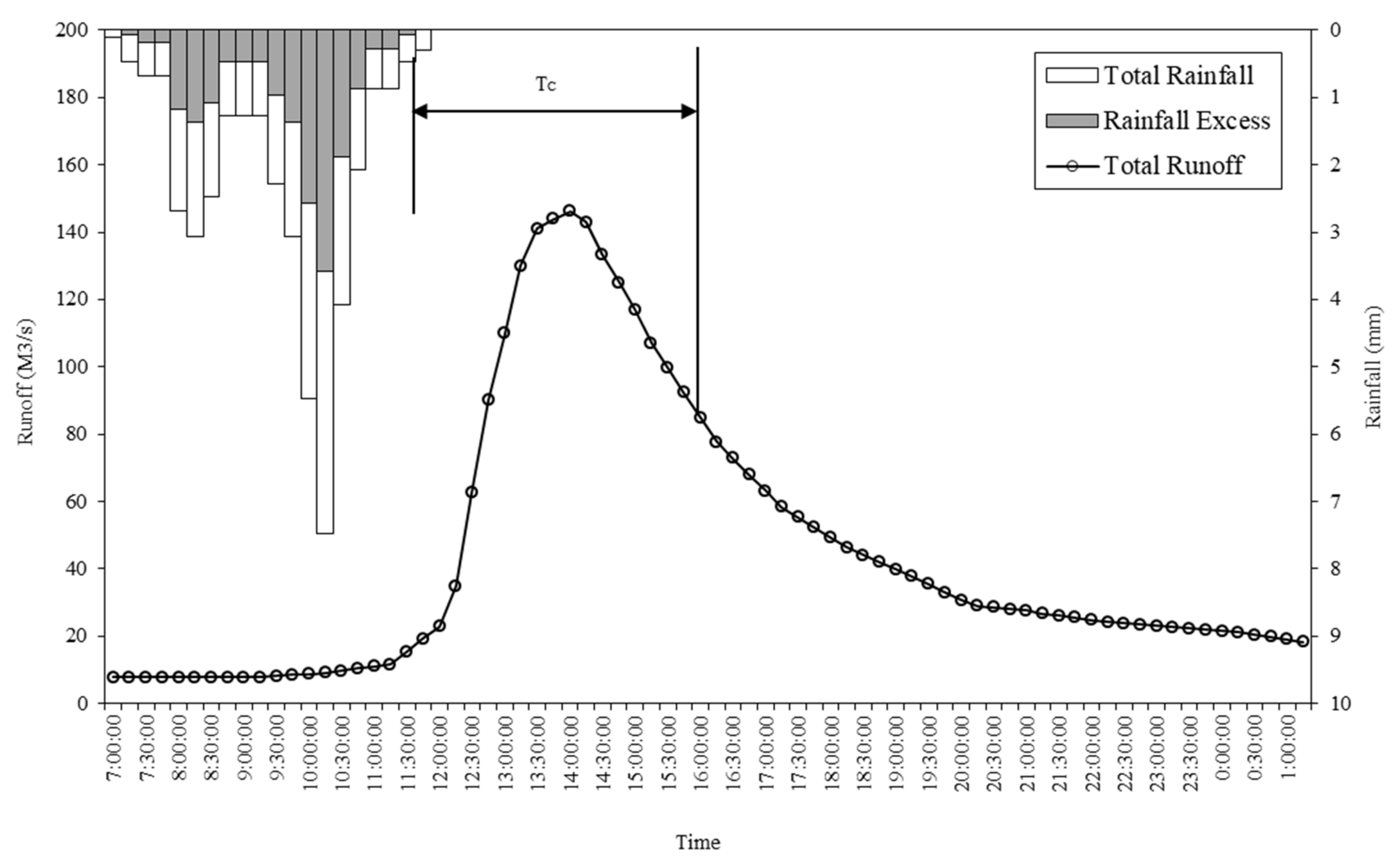
3.3. Graphical Method
3.4. Ranking and Improvement of Empirical Methods
| Method | Equation | Remarks |
|---|---|---|
| Bransby Williams (ASDOT 1995) | Developed for rural watersheds | |
| Kirpich (Tennessee) (1940) | Developed for small rural watersheds in Tennessee (0.004–0.453 Km2) and (0.03 < S < 0.1) | |
| Chow (1988) | Developed for rural watersheds in the USA (0.01–18.5 Km2) and (0.005 < Sc < 0.09) | |
| California Culverts Practice (CDH, 1960) | Developed for small mountainous watersheds in California | |
| Arizona DOT (1993) | Developed for agricultural watersheds Watershed area < 8.09 Km2 | |
| Johnstone-Cross (1949) | Developed for rural watersheds in the USA (64.8–4206.1 Km2) | |
| Temez (1987) | Developed for natural watersheds in Spain | |
| Haktanir and Sezen (1990) | Developed for watersheds in Turkey (11–9867 Km2) | |
| Giandotti (1934) | Developed for agricultural watersheds in central and northern Italy (170–70,000 Km2) | |
| Ventura (Mata-Lima et al., 2007) | Developed for rural watersheds in Italy | |
| Pilgrim and Mac Dermott (1982) | Developed for rural watersheds in eastern New South Wales | |
| Pasini (1914) | Developed for rural watersheds in Italy | |
| Williams (1922) | Developed for watersheds in India (Watershed area < 129.5 Km2) | |
| Dooge (1973) | Developed for rural watersheds in Ireland (145–948 Km2) | |
| Corps of Engineers (Linsley et al., 1977) | Developed for rural watersheds in the USA (Watershed area <12 Km2) |
4. Results and Discussion
4.1. Empirical Methods
4.2. Graphical Method
| Sub-Watershed | Event Number | Event Date | Rainfall Duration (h) | Rainfall Depth (mm) | Maximum Rainfall Intensity (mm/h) | Maximum Peak Flood (m3/s) | Tc (h) |
|---|---|---|---|---|---|---|---|
| Sikhoran | 1 | 4 November 2002 | 3.25 | 99 | 76 | 38 | 4.3 |
| 2 | 29 October 2003 | 9.5 | 29.2 | 14 | 95.5 | 4.5 | |
| 3 | 27 January 2004 | 2 | 17 | 29.6 | 13 | 4.5 | |
| 4 | 27 February 2010 | 6.5 | 38.5 | 36.4 | 10.1 | 4.5 | |
| 5 | 1 February 2013 | 9 | 40 | 12 | 24.4 | 3.8 | |
| 6 | 14 March 2014 | 7.5 | 29.1 | 65.2 | 391 | 4.5 | |
| 7 | 12 March 2015 | 14 | 32.9 | 16 | 20.3 | 3.8 | |
| 8 | 11 November 2015 | 15 | 41.4 | 17.6 | 25.2 | 4.0 | |
| 9 | 3 January 2016 | 4.75 | 15.9 | 15.2 | 28.7 | 4.3 | |
| Mean Tc | 4.2 | ||||||
| Shaghrud | 1 | 28 July 2007 | 2.5 | 13.2 | 24.8 | 19.6 | 5.8 |
| 2 | 30 March 2009 | 3.25 | 15.4 | 10 | 9.7 | 5.8 | |
| 3 | 31 March 2009 | 6.25 | 10.6 | 9.6 | 74.8 | 6.0 | |
| 4 | 8 November 2009 | 1.25 | 17 | 18.8 | 61.1 | 5.8 | |
| 5 | 3 March 2012 | 16 | 40 | 12.8 | 48.8 | 5.5 | |
| 6 | 3 March 2013 | 6.75 | 21.4 | 14.4 | 64.4 | 5.5 | |
| 7 | 12 March 2015 | 10.5 | 50 | 18.4 | 27 | 6.0 | |
| 8 | 26 February 2017 | 3 | 5.4 | 6.4 | 17.3 | 5.5 | |
| 9 | 20 March 2017 | 7.4 | 7.4 | 3.6 | 46.2 | 6.0 | |
| Mean Tc | 5.8 | ||||||
| Salubalm | 1 | 27 March 2003 | 3.5 | 24.8 | 74 | 13.8 | 5.0 |
| 2 | 15 January 2004 | 8.25 | 11.3 | 13.2 | 41.3 | 4.5 | |
| 3 | 20 February 2007 | 3.75 | 12.3 | 16 | 62.2 | 5.0 | |
| 4 | 17 March 2007 | 5.75 | 5 | 6 | 13.8 | 4.8 | |
| 5 | 27 October 2007 | 4 | 55.9 | 40.4 | 43 | 5.0 | |
| 6 | 30 March 2009 | 6.25 | 22.1 | 10.4 | 19.5 | 4.5 | |
| 7 | 8 December 2009 | 4.5 | 83.4 | 48.4 | 240 | 4.8 | |
| 8 | 9 December 2009 | 13.5 | 125 | 71.6 | 362 | 5.0 | |
| 9 | 5 February 2010 | 5 | 48.2 | 55.2 | 343 | 4.8 | |
| 10 | 21 January 2017 | 37.5 | 25.4 | 16 | 165 | 5.3 | |
| 11 | 25 March 2017 | 8.75 | 28.2 | 15.6 | 146 | 4.8 | |
| Mean Tc | 4.9 | ||||||
| Chahchkur | 1 | 30 March 2009 | 5.5 | 58.9 | 40.8 | 33.2 | 5.8 |
| 2 | 31 March 2009 | 4.5 | 44 | 29.6 | 49 | 5.3 | |
| 3 | 8 December 2009 | 5 | 34.8 | 48.2 | 34.9 | 5.3 | |
| 4 | 27 February 2010 | 7 | 34.9 | 12.4 | 151 | 4.8 | |
| Mean Tc | 5.3 | ||||||
4.3. Performance Evaluation of Empirical Methods in Sub-Watersheds
4.4. Regional Performance Evaluation of Empirical Methods
| Method | Difference% | |||
|---|---|---|---|---|
| Shaghrud | Sikhoran | Salubalm | Chahchakur | |
| Bransby Williams | 172 | 58 | 167 | 108 |
| Kirpich | −60 | −75 | −69 | −65 |
| Chow | 39 | −21 | 41 | 25 |
| California Culverts Practice | 12 | −50 | −11 | −43 |
| Arizona DOT | 29 | −26 | 21 | 9 |
| Johnstone-Cross | 70 | 18 | 78 | 60 |
| Temez | 134 | 45 | 127 | 88 |
| Haktanir and Sezen | 246 | 158 | 221 | 146 |
| Giandotti | −6 | −41 | −1 | 53 |
| Ventura | 328 | 65 | 249 | 301 |
| Pilgrim and Mac Dermott | 34 | 15 | 16 | 12 |
| Pasini | 381 | 79 | 310 | 329 |
| Williams | 9 | −37 | 7 | −17 |
| Dooge | 65 | 9 | 41 | 44 |
| Corps of Engineers | −38 | −62 | −40 | −50 |
4.5. Improving the Accuracy of the Top Methods
| Method | MAPE | RMSE | SE | R | Sum of Rankings |
|---|---|---|---|---|---|
| Bransby Williams | 135.49 | 7.64 | 245.60 | 0.831 | 49 |
| Rank | 12 | 12 | 12 | 13 | |
| Kirpich | 67.08 | 3.36 | −117.11 | 0.915 | 30 |
| Rank | 10 | 9 | 10 | 1 | |
| Chow | 34.22 | 1.86 | 44.80 | 0.840 | 27 |
| Rank | 6 | 6 | 6 | 9 | |
| California Culverts Practice | 24.99 | 1.45 | −26.31 | 0.826 | 28 |
| Rank | 5 | 5 | 4 | 14 | |
| Arizona DOT | 24.37 | 1.32 | 22.72 | 0.874 | 16 |
| Rank | 4 | 3 | 3 | 6 | |
| Johnstone-Cross | 59.02 | 3.37 | 106.92 | 0.834 | 38 |
| Rank | 9 | 10 | 9 | 10 | |
| Temez | 104.75 | 5.91 | 189.96 | 0.852 | 40 |
| Rank | 11 | 11 | 11 | 7 | |
| Haktanir and Sezen | 205.74 | 10.93 | 367.25 | 0.832 | 50 |
| Rank | 13 | 13 | 13 | 11 | |
| Giandotti | 19.35 | 1.33 | −8.11 | 0.678 | 22 |
| Rank | 2 | 4 | 1 | 15 | |
| Ventura | 234.70 | 13.87 | 432.53 | 0.901 | 45 |
| Rank | 14 | 14 | 14 | 3 | |
| Pilgrim and Mac Dermott | 21.85 | 1.31 | 39.53 | 0.885 | 15 |
| Rank | 3 | 2 | 5 | 5 | |
| Pasini | 277.60 | 16.27 | 510.42 | 0.891 | 49 |
| Rank | 15 | 15 | 15 | 4 | |
| Williams | 16.92 | 0.97 | −8.21 | 0.831 | 16 |
| Rank | 1 | 1 | 2 | 12 | |
| Dooge | 41.25 | 2.55 | 76.40 | 0.913 | 24 |
| Rank | 7 | 8 | 7 | 2 | |
| Corps of Engineers | 45.66 | 2.29 | −79.06 | 0.852 | 31 |
| Rank | 8 | 7 | 8 | 8 |
| Empirical Method | Original Equation | Modified Equation | Coefficient of Correlation | Mean Square Error (MSE) | Sum of Residuals |
|---|---|---|---|---|---|
| Williams | 0.918 | 0.06 | −7.1 × 10⁻¹⁵ | ||
| Pilgrim and Mac Dermott | 0.885 | 0.09 | −1.8 × 10⁻² | ||
| Arizona DOT | 0.915 | 0.06 | −3.1 × 10⁻¹⁰ |
| Sub-Watershed | Mean Tc Estimated by Graphical Method (h) | Modified Empirical Method | Tc Estimated by Modified Equation (h) | Difference% |
|---|---|---|---|---|
| Shaghrud | 5.8 | Modified Williams | 5.76 | −0.7 |
| Sikhoran | 4.2 | 4.24 | 0.9 | |
| Salubalm | 4.9 | 4.86 | −0.8 | |
| Chahchakur | 5.3 | 5.30 | 0 | |
| Shaghrud | 5.8 | Modified Pilgrim and Mac Dermott | 5.84 | 0.7 |
| Sikhoran | 4.2 | 4.38 | 4.2 | |
| Salubalm | 4.9 | 4.82 | −1.6 | |
| Chahchakur | 5.3 | 4.95 | −6.6 | |
| Shaghrud | 5.8 | Modified Arizona DOT | 5.77 | −0.5 |
| Sikhoran | 4.2 | 4.24 | 0.9 | |
| Salubalm | 4.9 | 4.86 | −0.8 | |
| Chahchakur | 5.3 | 5.30 | 0 |
4.6. Cross Validation for Overfitting
5. Limitations
6. Conclusions
Author Contributions
Funding
Institutional Review Board Statement
Informed Consent Statement
Data Availability Statement
Acknowledgments
Conflicts of Interest
References
- Schick, A.P. Hydrologic aspects of floods in extreme arid environments. Flood Geomorphol. 1988, 189–203. [Google Scholar]
- Zeng, X.; Zeng, X.; Barlage, M. Growing temperate shrubs over arid and semiarid regions in the Community Land Model-Dynamic Global Vegetation Model. Glob. Biogeochem. Cycles 2008, 22, 1–14. [Google Scholar] [CrossRef] [Green Version]
- Alinezhad, A.; Gohari, A.; Eslamian, S.; Baghbani, R. Uncertainty Analysis in Climate Change Projection Using Bayesian Approach. In Proceedings of the World Environmental and Water Resources Congress, Henderson, NV, USA, 17–21 May 2020; American Society of Civil Engineers: Henderson, NV, USA, 2020; pp. 167–174. [Google Scholar] [CrossRef]
- Pavlovic, S.B.; Moglen, G.E. Discretization Issues in Travel Time Calculation. J. Hydrol. Eng. 2008, 13, 71–79. [Google Scholar] [CrossRef]
- Bondelid, T.R.; McCuen, R.H.; Jackson, T.J. Sensitivity of SCS Models to Curve Number Variation1. JAWRA J. Am. Water Resour. Assoc. 1982, 18, 111–116. [Google Scholar] [CrossRef]
- Higgins, R.W.; Douglas, A.; Hahmann, A.; Berberry, E.H.; Gutzler, D.; Shuttleworth, J.; Stensrud, D.; Amador, J.; Carbone, R.; Cortez, M.; et al. Progress in Pan American CLIVAR research: The North American monsoon system. Atmosfera 2003, 16, 29–65. [Google Scholar]
- Azizian, A. Uncertainty Analysis of Time of Concentration Equations based on First-Order-Analysis (FOA) Method. Am. J. Eng. Appl. Sci. 2018, 11, 327–341. [Google Scholar] [CrossRef]
- Efstratiadis, A.; Koussis, A.D.; Koutsoyiannis, D.; Mamassis, N. Flood design recipes vs. reality: Can predictions for ungauged basins be trusted? Nat. Hazards Earth Syst. Sci. 2014, 14, 1417–1428. [Google Scholar] [CrossRef] [Green Version]
- Salimi, E.T.; Nohegar, A.; Malekian, A.; Hoseini, M.; Holisaz, A. Estimating time of concentration in large watersheds. Paddy Water Environ. 2017, 15, 123–132. [Google Scholar] [CrossRef]
- González-Álvarez, Á.; Molina-Pérez, J.; Meza-Zúñiga, B.; Viloria-Marimón, O.M.; Tesfagiorgis, K.; Mouthón-Bello, J.A. Assessing the performance of different time of concentration equations in urban ungauged watersheds: Case study of Cartagena de Indias, Colombia. Hydrology 2020, 7, 47. [Google Scholar] [CrossRef]
- Sharifi, S.; Hosseini, S.M. Methodology for Identifying the Best Equations for Estimating the Time of Concentration of Watersheds in a Particular Region. J. Irrig. Drain. Eng. 2011, 137, 712–719. [Google Scholar] [CrossRef] [Green Version]
- Perdikaris, J.; Gharabaghi, B.; Rudra, R. Reference Time of Concentration Estimation for Ungauged Catchments. Earth Sci. Res. 2018, 7, 58. [Google Scholar] [CrossRef]
- McCuen, R.H. Uncertainty Analyses of Watershed Time Parameters. J. Hydrol. Eng. 2009, 14, 490–498. [Google Scholar] [CrossRef]
- Beven, K. A history of the concept of time of concentration. Hydrol. Earth Syst. Sci. 2020, 24, 2655–2670. [Google Scholar] [CrossRef]
- McCuen, R.H.; Wong, S.L.; Rawls, W.J. Estimating Urban Time of Concentration. J. Hydraul. Eng. 1984, 110, 887–904. [Google Scholar] [CrossRef]
- Kaufmann de Almeida, I.; Kaufmann Almeida, A.; Garcia Gabas, S.; Alves Sobrinho, T. Performance of methods for estimating the time of concentration in a watershed of a tropical region. Hydrol. Sci. J. 2017, 62, 2406–2414. [Google Scholar] [CrossRef]
- Mudashiru, R.B.; Abustan, I.; Baharudin, F. Methods of Estimating Time of Concentration: A Case Study of Urban Catchment of Sungai Kerayong, Kuala Lumpur. Lect. Notes Civ. Eng. 2020, 53, 119–161. [Google Scholar] [CrossRef]
- Grimaldi, S.; Petroselli, A.; Tauro, F.; Porfiri, M. Time of concentration: A paradox in modern hydrology. Hydrol. Sci. J. 2012, 57, 217–228. [Google Scholar] [CrossRef] [Green Version]
- Dunne, T.; Black, R.D. Partial Area Contributions to Storm Runoff in a Small New England Watershed. Water Resour. Res. 1970, 6, 1296–1311. [Google Scholar] [CrossRef] [Green Version]
- Lim, T.C. Predictors of urban variable source area: A cross-sectional analysis of urbanized catchments in the United States. Hydrol. Process. 2016, 30, 4799–4814. [Google Scholar] [CrossRef]
- Kjeldsen, T.R.; Kim, H.; Jang, C.-H.; Lee, H. Evidence and Implications of Nonlinear Flood Response in a Small Mountainous Watershed. J. Hydrol. Eng. 2016, 21, 04016024. [Google Scholar] [CrossRef] [Green Version]
- Delleur, R.A.; Rao, R.A. Instantaneous unit hydrographs, peak discharges and time lags in urban basins. Hydrol. Sci. Bull. 1974, 19, 185–198. [Google Scholar] [CrossRef]
- Sharma, K.D.; Murthy, J.S.R. A practical approach to rainfall-runoff modelling in arid zone drainage basins. Hydrol. Sci. J. 1998, 43, 331–348. [Google Scholar] [CrossRef]
- Lange, J.; Leibundgut, C. Non-calibrated arid zone rainfall-runoff modelling. IAHS-AISH Publ. 2000, 45–52. [Google Scholar]
- Kirpich, Z.P. Time of concentration of small agricultural watersheds. Civ. Eng 1940, 10, 362. [Google Scholar]
- Singh, V.P. Hydrologic Systems: Rainfall-Runoff Modeling; Hydrologic Systems; Prentice Hall: Englewood Cliffs, NJ, USA, 1988; ISBN 9780134480510. [Google Scholar]
- Guermond, Y. The Modeling Process in Geography: From Determinism to Complexity, ISTE, 1st ed.; Wiley: Hoboken, NJ, USA, 2013; ISBN 9781118622575. [Google Scholar]
- Li, M.H.; Chibber, P. Overland flow time of concentration on very flat terrains. Transp. Res. Rec. 2008, 133–140. [Google Scholar] [CrossRef] [Green Version]
- Marek, M.A. Hydraulic Design Manual; Texas Department of Transportation (TxDOT): Austin, TX, USA, 2011.
- Pilgrim, D.H.; Chapman, T.G.; Doran, D.G. Problems of rainfall-runoff modelling in arid and semiarid regions. Hydrol. Sci. J. 1988, 33, 379–400. [Google Scholar] [CrossRef]
- Chow, V.T.; Maidment, D.R.; Mays, L.W. Applied Hydrology McGraw-Hill Book Company; MacGraw-Hill. Inc: New York, NY, USA, 1988. [Google Scholar]
- Fang, X.; Prakash, K. Revisit of NRCS unit hydrograph procedures. In Proceedings of the ASCE Texas Section Spring Meet, Austin, TX, USA, 2005; pp. 1–12. Available online: https://www.researchgate.net/publication/253038310_Revisit_of_NRCS_Unit_Hydrograph_Procedures (accessed on 17 September 2021).
- Fang, X.; Thompson, D.B.; Cleveland, T.G.; Pradhan, P.; Malla, R. Time of Concentration Estimated Using Watershed Parameters Determined by Automated and Manual Methods. J. Irrig. Drain. Eng. 2008, 134, 202–211. [Google Scholar] [CrossRef]
- Mateo Lázaro, J.; Sánchez Navarro, J.Á.; García Gil, A.; Edo Romero, V. Sensitivity analysis of main variables present in flash flood processes. Application in two Spanish catchments: Arás and Aguilón. Environ. Earth Sci. 2014, 71, 2925–2939. [Google Scholar] [CrossRef]
- Hadadin, N. Evaluation of several techniques for estimating stormwater runoff in arid watersheds. Environ. Earth Sci. 2013, 69, 1773–1782. [Google Scholar] [CrossRef]
- Chin, D.A. On relationship between curve numbers and phi indices. Water Sci. Eng. 2018, 11, 187–195. [Google Scholar] [CrossRef]
- McCuen, R.H. Hydrologic Analysis and Design, 4th ed.; Pearson: Upper Saddle River, NJ, USA; University of Maryland: College Park, MD, USA, 2017. [Google Scholar]
- Gupta, R.S. Hydrology and Hydraulic Systems, 4th ed.; Waveland Press: Long Grove, IL, USA, 2016; ISBN 1478634219. [Google Scholar]
- Singh, V.P. Elementary Hydrology; Prentice Hall: Englewood Cliffs, NJ, USA, 1992. [Google Scholar]
- American Society of Civil Engineers; Task Committee on Hydrology Handbook. Hydrology Handbook; ASCE: New York, NY, USA, 1996; ISBN 9780784470145. [Google Scholar]
- Linsley, R.K. Discussion of “Correlation of rainfall intensity and topography in Northern California. Eos, Trans. Am. Geophys. Union 1958, 39, 970–972. [Google Scholar] [CrossRef]
- Lopes, S.; Fragoso, M.; Lopes, A. Heavy rainfall events and mass movements in the funchal area (Madeira, Portugal): Spatial analysis and susceptibility assessment. Atmosphere 2020, 11, 104. [Google Scholar] [CrossRef] [Green Version]
- Legates, D.R.; McCabe Jr, G.J. Evaluating the use of “goodness-of-fit” measures in hydrologic and hydroclimatic model validation. Water Resour. Res. 1999, 35, 233–241. [Google Scholar] [CrossRef]
- Datafit Data Curve Fitting (Nonlinear Regression) and Data Plotting Software. 2009.
- Lever, J.; Krzywinski, M.; Altman, N. Points of significance: Model selection and overfitting. Nat. Methods 2016, 13, 703–705. [Google Scholar] [CrossRef]
- Wong, T.S. Assessment of Time of Concentration Formulas for Overland Flow. J. Irrig. Drain. Eng. 2005, 131, 383–387. [Google Scholar] [CrossRef]
- Sehler, R.; Li, J.; Reager, J.; Ye, H. Investigating Relationship Between Soil Moisture and Precipitation Globally Using Remote Sensing Observations. J. Contemp. Water Res. Educ. 2019, 168, 106–118. [Google Scholar] [CrossRef] [Green Version]
- Luo, W.; Harlin, J.M. A theoretical travel time based on watershed hypsometry. J. Am. Water Resour. Assoc. 2003, 39, 785–792. [Google Scholar] [CrossRef]
- Tucker, G.E.; Bras, R.L. Hillslope processes, drainage density, and landscape morphology. Water Resour. Res. 1998, 34, 2751–2764. [Google Scholar] [CrossRef] [Green Version]
- Pallard, B.; Castellarin, A.; Montanari, A. A look at the links between drainage density and flood statistics. Hydrol. Earth Syst. Sci. Discuss. 2008, 5, 2899–2926. [Google Scholar] [CrossRef]
- ASCE Task Committee on Definition of Criteria for Evaluation of Watershed Models of the Watershed Management Committee. Criteria for evaluation of watershed models. J. Irrig. Drain. Eng. 1993, 119, 429–442. [Google Scholar] [CrossRef]
- Vijai, G.H.; Soroosh, S.; Ogou, Y.P. Status of Automatic Calibration for Hydrologic Models: Comparison with Multilevel Expert Calibration. J. Hydrol. Eng. 1999, 4, 135–143. [Google Scholar] [CrossRef]
- Willmott, C.J.; Ackleson, S.G.; Davis, R.E.; Feddema, J.J.; Klink, K.M.; Legates, D.R.; O’donnell, J.; Rowe, C.M. Statistics for the evaluation and comparison of models. J. Geophys. Res. Ocean. 1985, 90, 8995–9005. [Google Scholar] [CrossRef] [Green Version]
- Zahraei, A.; Eslamian, S.; Rizi, A.S.; Azam, N.; Soltani, M.; Mousavi, M.; Pazdar, S.; Ostad-Ali-Askari, K. Mapping of Temperature Trend Slope in Iran′s Zayanderud River Basin: A Comparison of Interpolation Methods. Am. J. Eng. Appl. Sci. 2019, 12, 247–258. [Google Scholar] [CrossRef]
- Singh, J.; Knapp, H.V.; Arnold, J.G.; Demissie, M. Hydrological modeling of the Iroquois River watershed using HSPF and SWAT. J. Am. Water Resour. Assoc. 2005, 41, 343–360. [Google Scholar] [CrossRef]
- Moriasi, D.N.; Arnold, J.G.; Van Liew, M.W.; Bingner, R.L.; Harmel, R.D.; Veith, T.L. Model evaluation guidelines for systematic quantification of accuracy in watershed simulations. Trans. ASABE 2007, 50, 885–900. [Google Scholar] [CrossRef]
- KC, M.; Fang, X.; Yi, Y.-J.; Li, M.-H.; Thompson, D.B.; Cleveland, T.G. Improved Time of Concentration Estimation on Overland Flow Surfaces Including Low-Sloped Planes. J. Hydrol. Eng. 2014, 19, 495–508. [Google Scholar] [CrossRef]


| Method | Tc (h) | |||
|---|---|---|---|---|
| Shaghrud | Sikhoran | Salubalm | Chahchakur | |
| Bransby Williams | 15.8 | 6.6 | 13.1 | 11.0 |
| Kirpich | 2.3 | 1.0 | 1.5 | 1.8 |
| Chow | 8.1 | 3.3 | 6.9 | 6.6 |
| California Culverts Practice | 6.5 | 2.1 | 4.4 | 3.0 |
| Arizona DOT | 7.5 | 3.1 | 5.9 | 5.8 |
| Johnstone-Cross | 9.9 | 4.9 | 8.7 | 8.5 |
| Temez | 13.6 | 6.1 | 11.1 | 10.0 |
| Haktanir and Sezen | 20.1 | 10.8 | 15.7 | 13.1 |
| Giandotti | 5.5 | 2.5 | 4.8 | 8.1 |
| Ventura | 24.8 | 6.9 | 17.1 | 21.3 |
| Pilgrim and Mac Dermott | 7.8 | 4.8 | 5.7 | 5.9 |
| Pasini | 27.9 | 7.5 | 20.1 | 22.7 |
| Williams | 6.3 | 2.6 | 5.2 | 4.4 |
| Dooge | 9.5 | 4.6 | 6.9 | 7.6 |
| Corps of Engineers | 3.6 | 1.6 | 2.9 | 2.6 |
| Mean | 11.3 | 4.6 | 8.7 | 8.8 |
| Modified Methods | Variation of Coefficient of Correlation (Predicted R) | Mean Square Error (Predicted MSE) |
|---|---|---|
| Modified Williams | 0.904–0.925 | 0.09 |
| Modified Pilgrim and Mac Dermott | 0.871–0.912 | 0.10 |
| Modified Arizona DOT | 0.910–0.928 | 0.09 |
Publisher’s Note: MDPI stays neutral with regard to jurisdictional claims in published maps and institutional affiliations. |
© 2021 by the authors. Licensee MDPI, Basel, Switzerland. This article is an open access article distributed under the terms and conditions of the Creative Commons Attribution (CC BY) license (https://creativecommons.org/licenses/by/4.0/).
Share and Cite
Zahraei, A.; Baghbani, R.; Linhoss, A. Applying a Graphical Method in Evaluation of Empirical Methods for Estimating Time of Concentration in an Arid Region. Water 2021, 13, 2624. https://doi.org/10.3390/w13192624
Zahraei A, Baghbani R, Linhoss A. Applying a Graphical Method in Evaluation of Empirical Methods for Estimating Time of Concentration in an Arid Region. Water. 2021; 13(19):2624. https://doi.org/10.3390/w13192624
Chicago/Turabian StyleZahraei, Ali, Ramin Baghbani, and Anna Linhoss. 2021. "Applying a Graphical Method in Evaluation of Empirical Methods for Estimating Time of Concentration in an Arid Region" Water 13, no. 19: 2624. https://doi.org/10.3390/w13192624
APA StyleZahraei, A., Baghbani, R., & Linhoss, A. (2021). Applying a Graphical Method in Evaluation of Empirical Methods for Estimating Time of Concentration in an Arid Region. Water, 13(19), 2624. https://doi.org/10.3390/w13192624