Article

Regulation of Vegetation and Evapotranspiration by Water Level Fluctuation in Shallow Lakes

1
State Key Laboratory of Water Environment Simulation, School of Environment, Beijing Normal University, Beijing 100875, China
2
Key Laboratory for Water and Sediment Sciences, Ministry of Education, School of Environment, Beijing Normal University, Beijing 100875, China
3
Key Laboratory of Tibetan Environment Changes and Land Surface Processes, Institute of Tibetan Plateau Research, Chinese Academy of Sciences, Beijing 100101, China
*
Authors to whom correspondence should be addressed.
Water 2021, 13(19), 2651; https://doi.org/10.3390/w13192651
Submission received: 2 September 2021 / Revised: 24 September 2021 / Accepted: 24 September 2021 / Published: 26 September 2021

Abstract

:
Water level fluctuations play a critical role in regulating vegetation distribution, composition, cover and richness, which ultimately affect evapotranspiration. In this study, we first explore water level fluctuations and associated impacts on vegetation, after which we assess evapotranspiration (ET) under different water levels. The normalized difference vegetation index (NDVI) was used to estimate the fractional vegetation cover (Fv), while topography- and vegetation-based surface-energy partitioning algorithms (TVET model) and potential evaporation (Ev) were used to calculate ET and water evaporation (Ep). Results show that: (1) water levels were dramatically affected by the combined effect of ecological water transfer and climate change and exhibited significant decreasing trends with a slope of −0.011 m a−2; and (2) as predicted, there was a correlation between water level fluctuation at an annual scale with Phragmites australis (P. australis) cover and open-water area. Water levels also had a controlling effect on Fv values, an increase in annual water levels first increasing and then decreasing Fv. However, a negative correlation was found between Fv values and water levels during initial plant growth stages. (iii) ET, which varied under different water levels at an annual scale, showed different partition into transpiration from P. australis and evaporation from open-water area and soil with alterations between vegetation and open water. All findings indicated that water level fluctuations controlled biological and ecological processes, and their structural and functional characteristics. This study consequently recommends that specifically-focused ecological water regulations (e.g., duration, timing, frequency) should be enacted to maintain the integrity of wetland ecosystems for wetland restoration.

1. Introduction

Increases in the frequency and magnitude of climate extremes [1,2], over the past several decades, in combination with anthropogenic activities (e.g., water level changes from the reservoirs and dams throughout the world) have dramatically altered wetland hydrological regimes [3], leading to the widespread degradation of aquatic ecosystems at a global scale [4]. Alterations in hydrological regimes can result in a series of changes in physical, chemical and biological environments [5], as well as affecting the biota and ecosystems of shallow lakes [6,7]. Understanding interactions between hydrological regimes, biota and ecosystem processes can help maintain the integrity of wetlands and aid in wetland restoration [6,7,8].
Aquatic ecosystems reflect interactions between hydrology, geomorphology, ecology and biogeochemistry at different temporal and spatial scales [7,9]. Under the influence of climatic change and anthropogenic activity, hydrological regimes have deviated from their natural processes [6]. For example, dams, which contribute to water security, energy supply and flood protection, have fragmented freshwater species habitats [10], leading to connective shifts between hydrological regimes, organic matter and nutrients (e.g., [7,11]). Much effort has gone into prioritizing the restoration of aquatic ecosystems at a catchment scale (e.g., [6,9]). For example, ecological water transfer (inter-basin or inner-basin water diversion measures to maintain the environment flow or to meet ecological water requirements) is an approach used to restore changes in biological and ecological processes caused by hydrological regime variation and its associated effects on biota and ecosystem interactions. However, the outcome of such lake restoration projects may result in instability, occasionally causing lake systems to deviate in unforeseen directions [9,12]. Ecological water transfer projects tend to cause abrupt rises in water levels, which subsequently affect, and even cause, changes in the biological processes of wetlands [8]. For example, rising water levels resulting from ecological water transfer projects in the Ertou wetland have not been able to achieve expectant improvements to provide habitat for the Siberian crane (Grus leucogeranus) [13]. Although restoration projects play a critical role in restoring the connectivity of hydrological regimes and the interaction between biota and ecosystems, positive outcomes under increased biodiversity or the return to pre-disturbance community composition have rarely been documented [9]. This implies an inherent contradiction in the balance between restoration activities and natural environments. For example, hydrological regimes and associated biological and ecological interactions vary under natural conditions [6], while all such processes under restorative activities in most of cases are expected to be stable(i.e., maintaining water level steady). Accordingly, the objectives of this study were: (1) to explore temporal trends in annual water levels, and to address the impact of ecological water transfer projects on water levels; (2) to analyze water level effects on vegetation cover and the fractional vegetation cover (Fv); and (3) to assess variation in evapotranspiration (ET) under water level fluctuations. This will help us to better understand the effects of water level fluctuations on biological and ecosystem processes, while enabling us to enact suitable water management practices to maintain the integrity of wetland ecosystems.

2. Materials and Methods

2.1. Study Site

Baiyangdian Lake (38°43′–39°02′ N, 115°38′–116°07′ E), being the largest freshwater lake in the North China Plain (Figure 1), plays an important role in water resource provisions, flood controls and climate regime regulations [14]. Historically, nine rivers flowed into Baiyangdian Lake; however, most of these rivers, under the influence of climate change and anthropogenic activity, have dried up. Baiyangdian Lake belongs to a shallow-water lake system type, for which water levels range from 6.5 m to 9.5 m. When water levels fall below 6.5 m, Baiyangdian Lake will dry up, while its surrounding wetlands will disappear when the water levels fall below 5.5 m [15]. Furthermore, 94 km2 of raised fields and greater than 3700 ditches divide the entire water body into 140 small shallow lakes. Due to its unique wetland topography and vegetation composition (mainly P. australis community), small water level fluctuations typically cause significant alterations in ratio between vegetation cover and open-water area. To alleviate water shortages, ecological water transfer projects have been implemented in the lake since the 1980s to maintain its integrity [16]. Specifically, the planning outline of the Xiong’an New Area, which has jurisdiction over Baiyangdian Lake, includes an ordinance for its ecological restoration (e.g., natural water level fluctuating around 6.5 m, and water quality meeting China surface water environmental quality class III-IV standard). Inevitably, however, alterations in hydrological regimes will result in changes to Baiyangdian Lake aquatic ecosystems [17,18,19].

2.2. Data and Field Experiments

The MOD13Q1 Normalized Difference Vegetation Index (NDVI) was used to assess fractional vegetation cover (Fv) during 2001–2018, which was obtained from the Goddard Space Flight Center (https://ladsweb.modaps.eosdis.nasa.gov/, accessed on 18 January 2019). The MOD13Q1 NDVI product is a 16-day composite image of vegetation indices, in a sinusoidal projection, with a (nominal) spatial resolution of 250 m. Daily water level data throughout 1961–2018 were obtained from the Baoding Hydrological and Water Resources Survey Bureau, Hebei Province. Daily observations of air temperature, relative humidity, wind speed, and sunshine hours during the same period were obtained from Baoding meteorological station under the authority of the National Climatic Centre of the China Meteorological Administration (http://data.cma.cn, accessed on 18 January 2019). Combined with vegetation ecological characteristics (e.g., average height, and leaf area index-LAI), daily meteorological variables were used to obtain the total evapotranspiration (ET), potential transpiration (Tv), and potential evaporation (Ep) using the TVET mode and Penman equation [20,21].
Six quadrats (0.5 m × 0.5 m) were used to obtain the P. australis community’s parameters within the lake during growing season (from May to October during 2019), such as plant coverage, height, seedling number, and biomass in each month. The six quadrats were set at a depth from −10 cm to 50 cm at 10 cm intervals from the surface to the bottom of water, wherein 0 cm was the boundary between land and water. The relative elevations were also measured using the sounding rods, which were used to deduce the high-resolution DEM of the Baiyangdian wetland by combining the relative elevation and altitude data using ArcGIS 10.0. The DEM, combined with vegetation parameters, was used to deduce the suitable water level for the P. australis community, and then to simulate the dynamic vegetation pattern using the dynamic vegetation simulation model. Vegetation patterns obtained from the vegetation simulation model were compared with the patterns from landsat 8 satellite remote sensing images (August 2015), and validated its reliability.

2.3. Methods

(1) Temporal trend analysis method
To explore temporal trends in the data series, this study used a fitted linear regression model and the Mann–Kendall test to determine the slope of linear fitted lines as well as characteristics of abrupt changes. The fitted linear regression model, tested against the null hypothesis (slope) applying a two-tailed hypothesis test (t-test) at a confidence level of 95% [22], is a common method used today in statistical climate analysis [23]. Originally proposed by Mann (1945) [24] and refined by Kendall (1975) [25], the Mann–Kendall test has been widely used to evaluate the presence of statistically significant trends in hydrological and climatological time series (e.g., [23,26]) under the assumption of independence.
(2) Fractional vegetation cover
According to [27], the fractional vegetation cover (Fv) is approximately equal to the scaled normalized difference vegetation index (NDVI) (N*):
F v N *
N * = N D V I N D V I 0 N D V I s N D V I 0
where NDVI0 and NDVIs correspond to NDVI values of bare soil (LAI = 0) and surfaces with 100% Fv, respectively.
(3) Dynamic vegetation simulation model
Cellular automata, which are widely used to simulate vegetation species population dynamics (e.g., [8,28,29]), were used to simulate Phragmites australis variation patterns under water level fluctuations. Cellular automation is defined by S, N and f as follows [30]:
S t + 1 = f ( S t , N )
where S is a finite set representing the cell state; t denotes the transition step; f is the transition rule or function; and N is the amount of cell neighbors.
In this study, the vegetation parameters of each cell adopts a specific state, such as Sp.a, Sw and S0, representing the P. australis community, open-water area and arable or bare land area, which are sorted under a certain level of spatial distribution at the beginning of the simulation (St). Cell states during the subsequent time step (St+1) are then defined by wetland states and species interactions; namely, arable or bare land was defined as being in a stable state, while P. australis cover and open-water area could be present within each other’s cells under conditions of water level fluctuations, which can be summarized under the following rules:
S t + 1 = { S 0 ,   when   S t = S 0   and   W l < 0   cm S w ,   when   S t = S w   and   W l 60   cm S w ,   when   S t = S p . a   and   W l 60   cm S p . a ,   when   S t = S p . a , W l 60   cm S p . a ,   when   S t = S w , N p . a 5   and   W l 60   cm S w ,   when   S t = S 0   and   W l > 0   cm
where St and St+1 represent cell states at time t and t + 1, respectively; Np.a represents the cell number of the P. australis community; and Wl is water depth (cm).
To simulate P. australis cover and open-water area dynamics, 20 randomly-selected water levels were used to train the model, while natural water levels obtained between 1960 and 2019 were used to simulate vegetation pattern dynamics. Landsat vegetation pattern images of 2005 were used to validate simulation results from the dynamic vegetation model.
(4) Assessing evapotranspiration under water level fluctuations
To obtain ET under the 20 randomly-selected water levels, the Penman equation was used to calculate Ep [20], while vegetation-based surface energy partitioning algorithms (TVET model) combined with a dynamic vegetation model was used to estimate Ev and Tv in areas with vegetation cover.
The formula of the Penman equation is as follows [20]:
E p = E p R + E p A = Δ Δ + γ R n + γ Δ + γ 6430 ( 1 + 0.536 u 2 ) D λ
where Ep is potential evaporation (mm day−1); EpR (mm day−1) and EpA (mm day−1) represents radiative and aerodynamic components of the Penman equation, respectively; Rn is the daily net radiation (MJ m−2 day−1), wherein Rn/λ provides the equivalent water depth units (mm day−1) in this study; Δ is the slope of the saturation vapor pressure curve (Pa K−1); γ is the psychrometric constant (Pa K−1); D is the vapor pressure deficit (Pa); u2 is the daily average wind speed at 2 m height (m s−1); and λ is the latent heat of vaporization of water (2.45 × 10⁶ J kg−1).
The hybrid dual-source ET model by Guan and Wilson (2009) [21] has been used to partition ET into Ev and Tv (e.g., [8]). Guan and Wilson (2009) [21] and Liu et al. (2020) [8] provide details on TVET formulae as follows:
E v = Δ A s + ( 1 F r ) ρ a c p r a a + r a s ( e s ( T z ) e z ) Δ + γ
T v = Δ A c + F r ρ a c p r a c + r a a ( e s ( T z ) e z ) Δ + γ ( 1 + r s c r a c + r a a )
where total available energy (A) for the surface is first partitioned by a layer approach into two portions: the canopy part (Ac) and the soil part (As); ρa is the air density; cp is the specific heat capacity of air; es is the saturated vapor pressure; Δ represents the slope of the saturated vapor pressure versus the temperature curve; γ is the psychrometric constant (~66 Pa K−1); Tz is the air temperature at reference height z; r a a is the aerodynamic resistance between mean air flow at the canopy height and the reference height; r a s and r a c represent the aerodynamic resistance between the mean air flow at the canopy height and the soil surface, and the aerodynamic resistance between the mean leaf surface area to the mean canopy surface area, respectively; and r s c is the bulk canopy stomatal resistance.

3. Results

3.1. Alterations in Water-Fluctuations

Findings showed that the dynamic vegetation model yielded suitable results on P. australis cover patterns and open-water area, namely, an 84% agreement in image interpretation and a 0.75 Kappa coefficient (K) (Table 1).
Water level fluctuations, being influenced by both climate change and anthropogenic activity, exhibited a significant decreasing trend at a fitted linear regression slope of −0.011 m a−2 (p < 0.05) (Figure 2a). Annual water levels ranged from 5.43 to 9.22 m throughout 1960–2019. An abrupt downward change was detected in 1966, with an average annual water level of 8.78 and 7.39 m before and after the occurrence of abrupt change, respectively (Figure 2c). To meet ecological transfer water requirements, a series of ecological water transfer operations were conducted by government, which dramatically altered water levels. To reduce water consumption, some ecological water transfer operations were conducted outside the growing season. For example, water level increased from 6.72 to 7.47 m, which is equivalent to 93 × 106 m3 of water from the Yellow River flowing into the Baiyangdian wetland from December 2010 to March 2011. Therefore, ecological water transfer projects have dramatically altered water levels from the 1980s onwards.

3.2. Variation in Vegetation Patterns under Water Level Fluctuations

According to simulation results, P. australis cover and open-water area varied with water level fluctuations at an annual scale, whether they are in stable or dynamic states (Figure 3). Moreover, P. australis cover and open-water area decreased or increased with an increase in water levels, and vice versa. Given that the Baiyangdian wetland is a shallow lake system (wherein its lowest water level [6.5 m] is considered the tipping point after which the lake will dry up), changes in P. australis cover and open-water area are sensitive to increases or decreases in water levels. In this study, an abrupt change occurred at an approximate water level of 6.59 m, wherein P. australis area slopes were −46.24 and −1.91 km2 m−1 for water levels ranging from 5.43–6.59 and 6.59–9.50 m with decreasing of suitable water level for P. australis, respectively.
As seen in Figure 4, Fv values are controlled by water levels. The Fv increased, reaching a peak at a water level around 6.95 m, and then decreased along with water level increasing. According to the fitted model, the maximum Fv value (0.57) was deduced, and suitable water levels for vegetation ranged from 6.94 to 6.97 m. At a monthly scale, the linear relationship between Fv values and water levels were good in March and April, namely, the initial growing stage. And Fv decreased with an increase in water levels with a slope of −0.06 (R2 = 0.34).

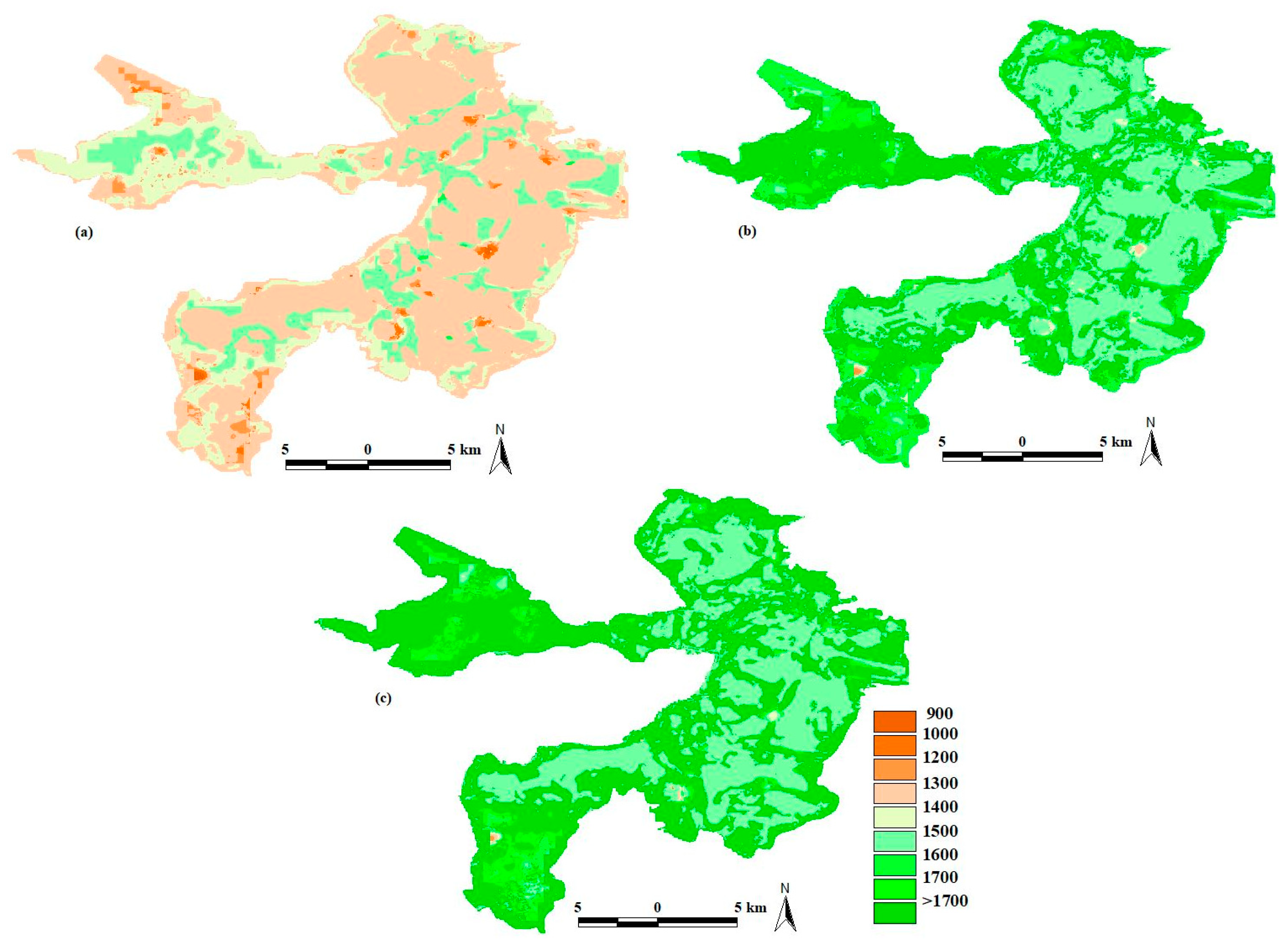
3.3. Evapotranspiration Variation under Water level Fluctuations

Alterations in vegetation patterns and Fv values changed ET at both monthly and annual scales. At an annual scale, ET, Ev, Tv and Ep exhibited decreasing trends with a slope of −3.52, −0.56, −2.97 and −2.70 mm a−2, respectively (Figure 5a). The Ev and Tv exhibited opposite trends, which was mainly caused by the controlling effects that vegetation cover has on partitioning net radiation and altering aerodynamics, wherein Tv reached a peak in July and Ev only yielded low values during this same month (Figure 5b). And ET values presented decreasing trends for the entire lake, open-water area and P. australis cover with a rate of −2.6, 1.4 and 1.2 × 10⁶ m3 a−2, respectively. Moreover, mean ET values for the entire lake, open-water area and P. australis cover were 398, 160 and 238 × 106 m3 a−1, respectively (Figure 5c).
Baiyangdian Lake ET has exhibited significant spatial variations over time (Figure 6). In 1965, when the water-level reached the maximum, ET ranged from 861 to 1506 mm a−1 with a spatial average value of 1278 mm a−1; in 1984, when the lake dried up, ET ranged from 1094 to 1925 mm a−1 with a spatial average value of 1628 mm a−1; and in 1998, when Fv reached the maximum, ET ranged from 1005 to 2129 mm a−1 with a spatial average value of 1732 mm a−1. Comparison between 1965, 1984 and 1998, water-level decreased first and increased later (from 9.22 to 6.37 to 7.15 m), however, spatially averaged ET kept increasing. Also, spatial difference of ET kept increasing (from 645 to 831 to 1124 mm a−1).

4. Discussion

4.1. Response of Ecological Effects to Water Level Fluctuations

Water levels have dramatically deviated from their natural regimes under the effects of climate changes and anthropogenic activities [6]. China has enacted ecological water transfer projects to alleviate water shortages (e.g., the Momoge, and Baiyangdian wetlands) [13,14]; however, such initiatives tend to cause abrupt wetland flooding events which result in a corresponding abrupt rise in water levels (as shown in Figure 2 and Figure 4). Water level fluctuations, particularly extreme ones, can disturb aquatic vegetation communities [31] and affect vegetation composition and distribution [32,33,34]. As shown in Figure 4, changes of Fr agreed with the water level fluctuation at annual and monthly scale. For example, prolonged deep flooding, caused by extreme climatic events or ecological water transfer projects, has resulted in a reduction of light infiltration that has subsequently contributed to the loss of both emergent and submerged aquatic vegetation [35,36,37]. As shown in Figure 4c, even small water level fluctuations during critical periods (e.g., the germination stage) will dramatically affect and alter the distribution of plant communities [23,38]. Meanwhile, affected by critical nutrient load thresholds, alterations in vegetation cover caused by extreme water level fluctuations have also been proven to play a vital role in controlling regime shifts [3,34]. Both increases and decreases in aquatic vegetation cover may led to increases and decreases in primary production as well as alterations in lake nutrient cycling processes [37], which will inevitably effect net primary productivity (NPP) and carbon (C) sequestration [39,40]. As shown in Figure 5 and Figure 6, water level fluctuations inevitably altered the ratio of vegetation cover and open water area, and correspondingly resulted in the changes in partition of ET. The causes mainly lie in changing physical and biological processes with macrophyte growth (e.g., P. australis). For example, macrophyte growth (e.g., height, leaf area for P. australis) influences aerodynamic resistance, and then alters the partition of solar radiation used for evaporation and transpiration [21], and even resulted in higher evapotranspiration than that for open water (Figure 5). On the other hand, vegetation regulates their physiological processes (i.e., photosynthesis, respiration and transpiration) to adapt to drought or flooding (e.g., [3,41]). Interestingly, ET for the Baiyangdian Lake increased at low water levels (e.g., Figure 6b) compared with that at high water levels (Figure 6a) due to P. australis expansion.

4.2. Implications for Wetland Restoration and Management

Diversity, vegetation structure and ecological processes, reported by Ruiz-Jaen and Aide (2005) [42], are the three ecological attributes used to assess the success of ecological restoration projects. Considering their critical role in maintaining wetland structure and function, several water regulation strategies have been enacted to alter hydrological regimes of wetlands, such as ecological water transfer projects (e.g., [13]) and water level controls (e.g., [3]). However, abrupt increases in water levels caused by such ecological water transfer projects and increases in minimum water levels both deviate from natural hydrological regimes (as shown in Figure 2d), which will inevitably alter aquatic vegetation communities and influence waterfowl habitats in the meantime (e.g., the Siberian crane) [13]. As reported by [7], it is important to increase our mechanistic understanding on how flow regimes impact biological and ecological processes to enact effective riverine restoration measures. In this context, although wetland restoration measures have been conducted in the recovery of hydrological and biological processes, such as ecological water transfer projects [13], soil and seed bank restoration approaches [43] and the incorporation of propagules [38], it is not sufficient to use hydrological or ecological processes alone to assess whether wetland restoration measures have been successful or not.
Understanding of nexus between flow-biota-ecosystem processes will help to resolve new challenges in assessing environmental flow [7] as well as providing a more comprehensive understanding of wetland restoration assessments. Furthermore, water level fluctuations can alter ecosystem metabolism, subsequently controlling both C and nutrient concentrations and flux [7]. Water level fluctuations, especially with regard to extreme drought or flooding, drive ecological and physiological processes while altering the C balance [44], which will also trigger ways in which shallow lakes react under C sequestration [3,45]. For example, it is important to understand (1) how many conditions affect vegetation distribution as well as its abundance, composition richness and diversity [46,47]; and (2) how many conditions alter anaerobic and aerobic states, and subsequently influence C decomposition and accumulation through means of hydrological regimes (e.g., water depth, duration, frequency and timing) [48,49]. Recently, much attention has been focused on the effects of extreme drought and flooding on C cycling processes (e.g., [6,44,50]. For example, ecosystem responses can exceed the duration of climate impacts through C cycle lag effects. And, most importantly, aquatic ecosystem response mechanisms to extreme hydrological regime alterations remain uncertain [44].

5. Conclusions

Water level fluctuations play a critical role in maintaining the ecosystem integrity of shallow lake systems. This study explored water level fluctuations, analyzed their influences on fractional vegetation cover (Fv), and simulated vegetation patterns and evapotranspiration (ET) under different water levels over time. Several conclusions can be drawn from our results:
(i) 
The average water levels at annual scale or during germination stage (e.g., March and April) play a key role in regulating the vegetation community. However, the abrupt rise in water levels (due to ecological water transfer) inevitably caused disturbances to aquatic vegetation communities.
(ii) 
The ET in different vegetation patterns influenced by water level fluctuations were estimated using the dynamic vegetation model combined with TVET model. Physical and biological processes influenced by varying macrophyte (e.g., P. australis) cover and open water area altered the partition of ET. Interestingly, high ET values appeared at low water levels instead of at high water levels.
(iii) 
Suitable water levels, estimated for maintaining suitable habitat for P. australis (avoiding abrupt changes in ratio of vegetation cover to open water area, and maintaining higher Fv), ranged from 6.59 to 6.97 m. Furthermore, ecological water transfer projects and operations should be regulated under a specific mode of operation to reduce their impact on macrophytes while maintaining the integrity of Baiyangdian Lake ecosystems, e.g., avoiding abrupt water level rise during the generation stage.

Author Contributions

Conceptualization, Q.L.; Methodology, L.L. and X.Y.; Validation, Q.L. and L.L.; Formal analysis, Q.L.; Investigation, X.Y.; M.L.; S.L. and S.Y.; Resources, X.W. and C.L.; Writing—original draft preparation, Q.L.; Writing—review and editing, Q.L. and L.L.; Project administration, Q.L. All authors have read and agreed to the published version of the manuscript.

Funding

This study was supported by the Major Science and Technology Program for Water Pollution Control and Treatment (No. 2018ZX07110001), the National Natural Science Foundation of China (No. 42071129, 41771042, 51579008).

Institutional Review Board Statement

Not applicable.

Informed Consent Statement

Not applicable.

Data Availability Statement

The water level data used in this study are not publicly available due to management requirement of Baoding Hydrological and Water Resources Survey Bureau, Hebei Province, but are available from the corresponding author. The meteorological data was obtained from China Meteorological Data Service Center (http://data.cma.cn, accessed on 19 January 2019). All data generated or analyzed during this study are included in this published paper.

Acknowledgments

The authors would like to thank the National Climatic Center of the China Meteorological Administration for providing the meteorological data. The authors would also like to thank the Baoding Hydrological and Water Resources Survey Bureau, Hebei Province, for providing the hydrological data. We thank the Editor and the two anonymous reviewers for comments that substantially improved this manuscript.

Conflicts of Interest

The authors declare no conflict of interest.

References

  1. Ponce-Campos, G.E.; Moran, M.S.; Huete, A.; Zhang, Y.; Bresloff, C.; Huxman, T.E.; Eamus, D.; Bosch, D.D.; Buda, A.R.; Gunter, S.A.; et al. Ecosystem resilience despite large-scale altered hydroclimatic conditions. Nature 2013, 494, 349–352. [Google Scholar] [CrossRef]
  2. Knapp, A.K.; Hoover, D.L.; Wilcox, K.R.; Avolio, M.L.; Koerner, S.E.; La Pierre, K.J.; Loik, M.E.; Luo, Y.Q.; Sala, O.; Smith, M.D. Characterizing differences in precipitation regimes of extreme wet and dry years: Implications for climate change experiments. Glob. Chang. Biol. 2015, 21, 2624–2633. [Google Scholar] [CrossRef] [Green Version]
  3. Kong, X.; He, Q.; Yang, B.; He, W.; Xu, F.; Janssen, A.B.; Kuiper, J.J.; van Gerven, L.A.; Qin, N.; Jiang, Y.J.; et al. Hydrological regulation drives regime shifts: Evidence from paleolimnology and ecosystem modeling of a large shallow Chinese lake. Glob. Chang. Biol. 2017, 23, 737–754. [Google Scholar] [CrossRef] [PubMed]
  4. Reid, W.V.; Mooney, H.A.; Cropper, A.; Capistrano, D.; Zurek, M.B. Millennium Ecosystem Assessment; Synthesis Report; Island Press: Washington, DC, USA, 2005. [Google Scholar]
  5. Poff, N.L.; Allan, J.D.; Bain, M.B.; Karr, J.R.; Prestegaard, K.L.; Richter, B.D.; Sparks, R.E.; Stromberg, J.C. The Natural Flow Regime. Bioscience 1997, 47, 769–784. [Google Scholar] [CrossRef]
  6. Poff, N.L. Beyond the natural flow regime? Broadening the hydro-ecological foundation to meet environmental flows challenges in a non-stationary world. Freshw. Biol. 2018, 63, 1011–1021. [Google Scholar] [CrossRef]
  7. Palmer, M.; Ruhi, A. Linkages between flow regime, biota, and ecosystem processes: Implications for river restoration. Science 2019, 365, eaaw2087. [Google Scholar] [CrossRef] [Green Version]
  8. Liu, Q.; Liu, J.; Liu, H.; Liang, L.; Cai, Y.; Wang, X.; Li, C. Vegetation dynamics under water-level fluctuations: Implications for wetland restoration. J. Hydrol. 2020, 581, 124418. [Google Scholar] [CrossRef]
  9. Polvi, L.E.; Lind, L.; Persson, H.; Miranda-Melo, A.; Pilotto, F.; Su, X.; Nilsson, C. Facets and scales in river restoration: Nestedness and interdependence of hydrological, geomorphic, ecological, and biogeochemical processes. J. Environ. Manag. 2020, 265, 110288. [Google Scholar] [CrossRef] [PubMed]
  10. Barbarossa, V.; Schmitt, R.J.P.; Huijbregts, M.A.J.; Zarfl, C.; King, H.; Schipper, A.M. Impacts of current and future large dams on the geographic range connectivity of freshwater fish worldwide. Proc. Natl. Acad. Sci. USA 2020, 117, 3648–3655. [Google Scholar] [CrossRef] [Green Version]
  11. Li, G.; Wang, X.T.; Yang, Z.; Mao, C.; West, A.J.; Ji, J. Dam-triggered organic carbon sequestration makes the Changjiang (Yangtze) river basin (China) a significant carbon sink. J. Geophys. Res. Biogeosci. 2015, 120, 39–53. [Google Scholar] [CrossRef]
  12. Scheffer, M.; Carpenter, S.; Foley, J.A.; Folke, C.; Walker, B. Catastrophic shifts in ecosystems. Nature 2001, 413, 591–596. [Google Scholar] [CrossRef] [PubMed]
  13. Jiang, H.B.; Wen, Y.; Zou, L.F.; Wang, Z.Q.; He, C.G.; Zou, C.L. The effects of a wetland restoration project on the Siberian crane (Grus leucogeranus) population and stopover habitat in Momoge National Nature Reserve, China. Ecol. Eng. 2016, 96, 170–177. [Google Scholar] [CrossRef]
  14. Wang, Q.; Yang, Z.F.; Liu, Q.; Zhao, Y. Water preservation and the ecological effects of removing leaves from stalks for a reed dominant wetland. Ecol. Eng. 2012, 49, 118–122. [Google Scholar] [CrossRef]
  15. Cui, B.; Li, X.; Zhang, K. Classification of hydrological conditions to assess water allocation schemes for Lake Baiyangdian in North China. J. Hydrol. 2010, 385, 247–256. [Google Scholar] [CrossRef]
  16. Liu, Q. Effects of groundwater level fluctuation on Phragmites australis evapotranspiration in the Baiyangdian Lake. Wetl. Sci. 2014, 12, 552–558. [Google Scholar]
  17. Zhao, Y.; Yang, Z.; Xia, X.; Wang, F. A shallow lake remediation regime with Phragmites australis: Incorporating nutrient removal and water evapotranspiration. Water Res. 2012, 46, 5635–5644. [Google Scholar] [CrossRef]
  18. Li, X.; Cui, B.; Yang, Q.; Lan, Y. Impacts of water level fluctuations on detritus accumulation in Lake Baiyangdian, China. Ecohydrology 2016, 9, 52–67. [Google Scholar] [CrossRef]
  19. Wang, Q.; Yan, D.; Yuan, Y.; Wang, D. Study on the Quantification of Drought in Freshwater Wetlands—A Case Study in Baiyangdian Wetland. Wetlands 2014, 34, 1013–1025. [Google Scholar] [CrossRef]
  20. Shuttleworth, W.J. Evaporation. In Handbook of Hydrology; Maidment, D.R., Ed.; McGraw-Hill: New York, NY, USA, 1993; Chapter 4. [Google Scholar]
  21. Guan, H.D.; Wilson, J.L. A hybrid dual-source model for potential evaporation and transpiration partitioning. J. Hydrol. 2009, 377, 405–416. [Google Scholar] [CrossRef]
  22. Serrano, A.; Mateos, V.L.; García, J.A. Trend analysis of monthly precipitation over the Iberian Peninsula for the period 1921–1995. Phys. Chem. Earth B 1999, 24, 85–90. [Google Scholar] [CrossRef]
  23. Liu, Q.; Yang, Z. Quantitative estimation of the impact of climate change on actual evapotranspiration in the Yellow River Basin, China. J. Hydrol. 2010, 395, 226–234. [Google Scholar] [CrossRef]
  24. Mann, H.B. Non-parametric test against trend. Econometrika 1945, 13, 245–259. [Google Scholar] [CrossRef]
  25. Kendall, M.G. Rank Correlation Methods; Charles Griffin: London, UK, 1975. [Google Scholar]
  26. Birsan, M.-V.; Molnar, P.; Burlando, P.; Pfaundler, M. Streamflow trends in Switzerland. J. Hydrol. 2005, 314, 312–329. [Google Scholar] [CrossRef]
  27. Carlson, T.N.; Ripley, D.A. On the relation between NDVI, fractional vegetation cover, and leaf area index. Remote Sens. Environ. 1997, 62, 241–252. [Google Scholar] [CrossRef]
  28. Huang, H.M.; Zhang, L.Q.; Guan, Y.J.; Wang, D.H. A cellular automata model for population expansion of Spartina alterniflora at Jiuduansha Shoals, Shanghai, China. Estuar. Coast. Shelf Sci. 2008, 77, 47–55. [Google Scholar] [CrossRef]
  29. Qi, M.; Sun, T.; Xue, S.; Yang, W.; Shao, D.; Martinez-Lopez, J. Competitive ability, stress tolerance and plant interactions along stress gradients. Ecology 2018, 99, 848–857. [Google Scholar] [CrossRef] [PubMed]
  30. Wolfram, S. Universality and complexity in cellular automata. Phys. D Nonlinear Phenom. 1984, 10, 1–35. [Google Scholar] [CrossRef]
  31. Foti, R.; del Jesus, M.; Rinaldo, A.; Rodriguez-Iturbe, I. Signs of critical transition in the Everglades wetlands in response to climate and anthropogenic changes. Proc. Natl. Acad. Sci. USA 2013, 110, 6296–6300. [Google Scholar] [CrossRef] [Green Version]
  32. Budelsky, R.A.; Galatowitsch, S.M. Effects of water regime and competition on the establishment of a native sedge in restored wetlands. J. Appl. Ecol. 2000, 37, 971–985. [Google Scholar] [CrossRef]
  33. Wilcox, D.A.; Nichols, S.J. The effects of water-level fluctuations on vegetation in a Lake Huron wetland. Wetlands 2008, 28, 487–501. [Google Scholar] [CrossRef]
  34. Schooler, S.S.; Salau, B.; Julien, M.H.; Ives, A.R. Alternative stable states explain unpredictable biological control of Salvinia molesta in Kakadu. Nature 2011, 470, 86–89. [Google Scholar] [CrossRef]
  35. van der Valk, A.G. Effects of prolonged flooding on the distribution and biomass of emergent species along a freshwater wetland coenocline. Vegetatio 1994, 110, 185–196. [Google Scholar] [CrossRef]
  36. Havens, K.E.; Fox, D.; Gornak, S.; Hanlon, C. Aquatic vegetation and largemouth bass population responses to water-level variations in Lake Okeechobee, Florida (USA). Hydrobiologia 2005, 539, 225–237. [Google Scholar] [CrossRef]
  37. Zhang, Y.L.; Jeppesen, E.; Liu, X.H.; Qin, B.Q.; Shi, K.; Zhou, Y.Q.; Thomaz, S.M.; Deng, J.M. Global loss of aquatic vegetation in lakes. Earth-Sci. Rev. 2017, 173, 259–265. [Google Scholar] [CrossRef]
  38. An, Y.; Gao, Y.; Tong, S.Z. Emergence and growth performance of Bolboschoenus planiculmis varied in response to water level and soil planting depth: Implications for wetland restoration using tuber transplantation. Aquat. Bot. 2018, 148, 10–14. [Google Scholar] [CrossRef]
  39. Jacinthe, P.A. Carbon dioxide and methane fluxes in variably-flooded riparian forests. Geoderma 2015, 241, 41–50. [Google Scholar] [CrossRef]
  40. Ye, X.C.; Meng, Y.K.; Xu, L.G.; Xu, C.Y. Net primary productivity dynamics and associated hydrological driving factors in the floodplain wetland of China’s largest freshwater lake. Sci. Total Environ. 2019, 659, 302–313. [Google Scholar] [CrossRef] [PubMed]
  41. Yang, Y.; Guan, H.; Batelaan, O.; McVicar, T.R.; Long, D.; Piao, S.; Liang, W.; Liu, B.; Jin, Z.; Simmons, C.T. Contrasting responses of water use efficiency to drought across global terrestrial ecosystems. Sci. Rep. 2016, 6, 23284. [Google Scholar] [CrossRef] [Green Version]
  42. Ruiz-Jaen, M.C.; Aide, T.M. Restoration Success: How Is It Being Measured? Restor. Ecol. 2005, 13, 569–577. [Google Scholar] [CrossRef]
  43. Bossuyt, B.; Honnay, O. Can the seed bank be used for ecological restoration? An overview of seed bank characteristics in European communities. J. Veg. Sci. 2008, 19, 875–884. [Google Scholar] [CrossRef]
  44. Frank, D.; Reichstein, M.; Bahn, M.; Thonicke, K.; Frank, D.; Mahecha, M.D.; Smith, P.; van der Velde, M.; Vicca, S.; Babst, F.; et al. Effects of climate extremes on the terrestrial carbon cycle: Concepts, processes and potential future impacts. Glob. Chang. Biol. 2015, 21, 2861–2880. [Google Scholar] [CrossRef] [Green Version]
  45. Dong, X.; Anderson, N.J.; Yang, X.; Chen, X.; Shen, J. Carbon burial by shallow lakes on the Yangtze floodplain and its relevance to regional carbon sequestration. Glob. Chang. Biol. 2012, 18, 2205–2217. [Google Scholar] [CrossRef]
  46. Sánchez-Carrillo, S.; Angeler, D.G.; Sanchez-Andres, R.; Alvarez-Cobelas, M.; Garatuza-Payan, J. Evapotranspiration in semi-arid wetlands: Relationships between inundation and the macrophyte-cover: Open-water ratio. Adv. Water Resour. 2004, 27, 643–655. [Google Scholar] [CrossRef]
  47. Midwood, J.D.; Chow-Fraser, P. Changes in aquatic vegetation and fish communities following 5 years of sustained low water levels in coastal marshes of eastern Georgian Bay, Lake Huron. Glob. Chang. Biol. 2012, 18, 93–105. [Google Scholar] [CrossRef]
  48. Blodau, C.; Moore, T.R. Experimental response of peatland carbon dynamics to a water table fluctuation. Aquat. Sci. Res. Across Boundaries 2003, 65, 47–62. [Google Scholar] [CrossRef]
  49. Chimner, R.A.; Pypker, T.G.; Hribljan, J.A.; Moore, P.A.; Waddington, J.M. Multi-decadal Changes in Water Table Levels Alter Peatland Carbon Cycling. Ecosystems 2016, 20, 1042–1057. [Google Scholar] [CrossRef]
  50. Reich, P.; Lake, P.S. Extreme hydrological events and the ecological restoration of flowing waters. Freshw. Biol. 2015, 60, 2639–2652. [Google Scholar] [CrossRef]
Figure 1. Baiyangdian Lake location.
Water 13 02651 g001
Figure 2. The temporal variation of water level for Baiyangdian wetland. (a) temporal trend for water level; (b) abrupt changes for water level detected by the Mann-Kendall method; and (c) a water level fluctuation example caused by the ecological water transfer from December 2010 to March 2011. The u represents statistics variables in the Mann-Kendall method, C1 and C2 is statistical variables calculated from normal and invert series. The intersection point of C1 and C2 located between the confidence lines (±1.96 at 95% confidence line) is the time of the abrupt changes [24,25].
Water 13 02651 g002
Figure 3. The variation of P. australis cover and open water area with water level fluctuations. (a) P. australis cover (showed as ) and open water area (presented as ) varied with water level fluctuations; (b) the abrupt changes detected by Mann-Kendall method for P. australis cover.
Water 13 02651 g003
Figure 4. Fractional vegetation cover (Fv) alterations under water level fluctuations at an annual scale (a) and monthly scale (b), and in March and April (c) which yielded the highest overall Fv values.
Water 13 02651 g004
Figure 5. Variation in annual (a) and monthly (b) evapotranspiration (ET) and potential evaporation (Ev), potential evaporation (Ev), potential transpiration (Tv) and potential evaporation (Ep) in Baiyangdian Lake. Annual evapotranspiration (ET) for reed, open water, and whole lake showed (c). This figure also provides linear fitted slopes for ET, Ev, Tv and Ep and for ET for the entire lake and open-water area and P. australis cover.
Water 13 02651 g005
Figure 6. Evapotranspiration (ET) variation in Baiyangdian Lake under three different historical water levels: (a) the maximum water level (9.22 m, in 1965), (b) the water level wherein the lake dried up (6.37 m, in 1984) and (c) the maximum fractional vegetation cover (Fv) (7.15 m, in 1998).
Water 13 02651 g006
Table 1. Comparation for vegetation pattern between simulated by vegetation simulated model and interpreted from landsat data (2015).
ClassificationP. australisOpen-Water AreaOther Land-Use TypesTotalAccuracy (%)
P. australis129,27511,6070140,88291.76
Open-water area38,81973,8940112,71365.56
Other land-use types3018114182,50286,66195.20
Total171,11286,64282,502
Accuracy (%)75.5585.29100
Overall accuracy84% Kappa0.75
Publisher’s Note: MDPI stays neutral with regard to jurisdictional claims in published maps and institutional affiliations.

