Numerical Investigation of Hydraulics in a Vertical Slot Fishway with Upgraded Configurations

Abstract

The implementation of vertical slot fishway (VSF) has been demonstrated to be an effective mitigation measure to alleviate extensive river fragmentation by artificial hydraulic structures such as weirs and dams. However, non-suitable flow velocity and turbulent kinetic energy significantly affect fish swimming behavior and, as a result, hinder such facilities’ performance. Therefore, this study’s main objective is to propose a new configuration of VSF that can allow the passage of different fish species under frequent variations of flow discharge. To achieve that objective several novel configurations of VSF were numerically investigated using the FLOW-3D^® model. Namely, five variants of angles between baffles, four different pool widths, and another upgraded version of VSF by introducing cylindrical elements positioned after the opening behind the baffles were tested. Results show that smaller angles between baffles increase the Vmax and decrease the maximum turbulent kinetic energy (TKE_max); the opposite result was obtained when increasing angles between baffles. Namely, the Vmax was increased up to 17.9% for α = 0° and decreased up to 20.37% for α = 37°; in contrast, TKE_max decreased up to −20% for α = 0° and increased up to 26.5% for α = 37°. Narrowing the pool width increased the Vmax linearly; nevertheless, it did not significantly affect the TKE_max as the maximum difference was only +3.5%. Using cylinders with a large diameter decreased the Vmax and increased TKE_max; in contrast, using cylinders with smaller diameters further reduced the Vmax velocity inside the pool while increasing the TKE_max. However, in the case of cylinders, the dimension of the recirculation depended on the configuration and arrangement of the cylinder within the pool. Overall, the maximum velocity was reached at near 77% of the water depth in all cases. Finally, solution-oriented findings resulted from this study would help water engineers to design cost-effective VSF fishways to support the sustainable development of hydraulic structures while preserving aquatic biodiversity.

1. Introduction

For decades, dams have been built for multiple purposes, such as irrigation, water supply, navigation and fish farming, flood control, recreation, and energy generation [1,2]. In recent years, hydropower, including both small and large examples, has attained an increasingly significant role within available renewable energy sources, currently representing the most significant contributor of its kind to power generation, especially in Europe, and is also gaining tremendous attention in developing countries, as well [3,4]. Due to its technical-economic specificities, hydropower is becoming a key player in helping to face global energy challenges, fighting climate change, and achieving sustainable development goals (SDGs). Although hydropower plants are considered relatively clean in terms of gas emissions, they cause direct or indirect ecological impacts on river ecosystems by altering the natural flow regime, degrading water quantity and quality, impairing the aquatic habitats and connectivity [5,6]. The latter, aquatic habitats degradation and especially loss of longitudinal connectivity, are among the major impacts induced by almost all types of hydropower plants [4,7]. Despite the many economic benefits that dams and hydropower plants provide, the conservation of aquatic ecosystems should not be compromised. The conservation of aquatic ecosystems is vital to safeguard the aquatic biota and provide immense essential benefits to humans [8]. The extensive development of hydropower plants has already considerably modified freshwater ecosystems at many rivers worldwide [4,9]. Therefore, it is imperative to develop a cost-effective and sustainable solution to avoid or mitigate the ecological impacts of dams, especially hydropower plants. As loss of longitudinal connectivity is one of the major impacts of hydropower plants, there have been considerable efforts to mitigate this impact by developing fishways [10,11,12,13,14]. Fishways enable fish to maintain migrations through hydraulic structures, re-establish migrations in case of prolonged blockage at artificial barriers, and/or facilitate migrations upstream/downstream of natural barriers, as well [15].

Swimming ability is a crucial factor in successful fish migrations. In natural conditions, fish migrating upstream need to navigate through various hydraulic conditions of the flow discharge. The hydraulic conditions range from areas of slow currents, such as pools, broad river sections, or reaches of mild stream gradients, to areas of fast currents, such as rapids, narrow sections, or reaches with steep gradients [15]. Therefore, any fishway design should mimic the hydraulic conditions of habitats and geomorphological units found in natural rivers [10,16]. Because of their technical specificity, pool, and weir-type, fishways are the most common fish pass used to facilitate the upstream movement of fish [17,18]. Given their advantage to handle broad variations in water levels, Vertical Slot Fishways (VSF) remains among the most effective pool-type fishways [15,19]. Turbulence, namely turbulent kinetic energy and flow velocity, are the main hydraulic variables that influence fish swimming ability most [12,20]. Particularly, turbulence, demarcated as a three-dimensional hydraulic parameter, which varies in time and space, may attract or prevent fish migratory movements [21]. High turbulences not only prevent fish migration but may also cause bodily injuries or even fish mortality [10,21,22,23]. Turbulent eddies are a frequent hydraulic phenomenon occurring in natural aquatic habitats and pool-type fishways, including the VSF. This type of pool fishway is usually very effective in ensuring the unhindered passage of the target species (i.e., mainly sea trout (Salmo trutta), salmon (Salmo salar), shad, and marine lamprey (Petromyzon marinus)) and several riverine species, such as trout and grayling (Thymallus thymallus), barbel (Barbus), and bream (Abramis brama) [19,24]. However, observations have shown that undesirable hydraulic conditions, such as large eddies, hinder some small fish species’ ability to pass safely through large pools. While in natural aquatic habitats, fish have various options of choosing the most suitable habitat and avoiding high turbulent zones, in contrast, in a fishway, the frequent occurrence of turbulent eddies may jeopardize its functionality [11,19,22]. Therefore, to date, to avoid such undesirable hydraulic conditions and improve the fishway effectiveness, different configurations of VSF have been developed considering the slot layout optimization [22,25], pool depth optimization [26], introducing several slots to improve the entrance attractiveness for fish [13], turning pools in stepped fishways [27], and testing different slots position, among others [28]. In general, each newly proposed configuration of VSF is designed considering the swimming ability of specific fish species. However, considering the impact of climate change on freshwater availability and variability and several technical-economic aspects, it is imperative to develop a configuration of VSF that could cope with such conditions and facilitate the migration of different fish species.

Nevertheless, no study has investigated such a comprehensive VSF configuration to the best of the authors’ knowledge. Therefore, this study’s main objective is to numerically investigate the performance of the different VSF configurations and, finally, propose the best option regarding the fish migration effectiveness. The rest of the manuscript is organized as follows: Section 2 gives a detailed description of the tested VSF configuration and hydrodynamic modeling; Section 3 presents the main results and discusses the relevance and effectiveness of each tested VSF configuration. Finally, the main conclusions drawn from this study are presented in Section 4.

2. Materials and Methods

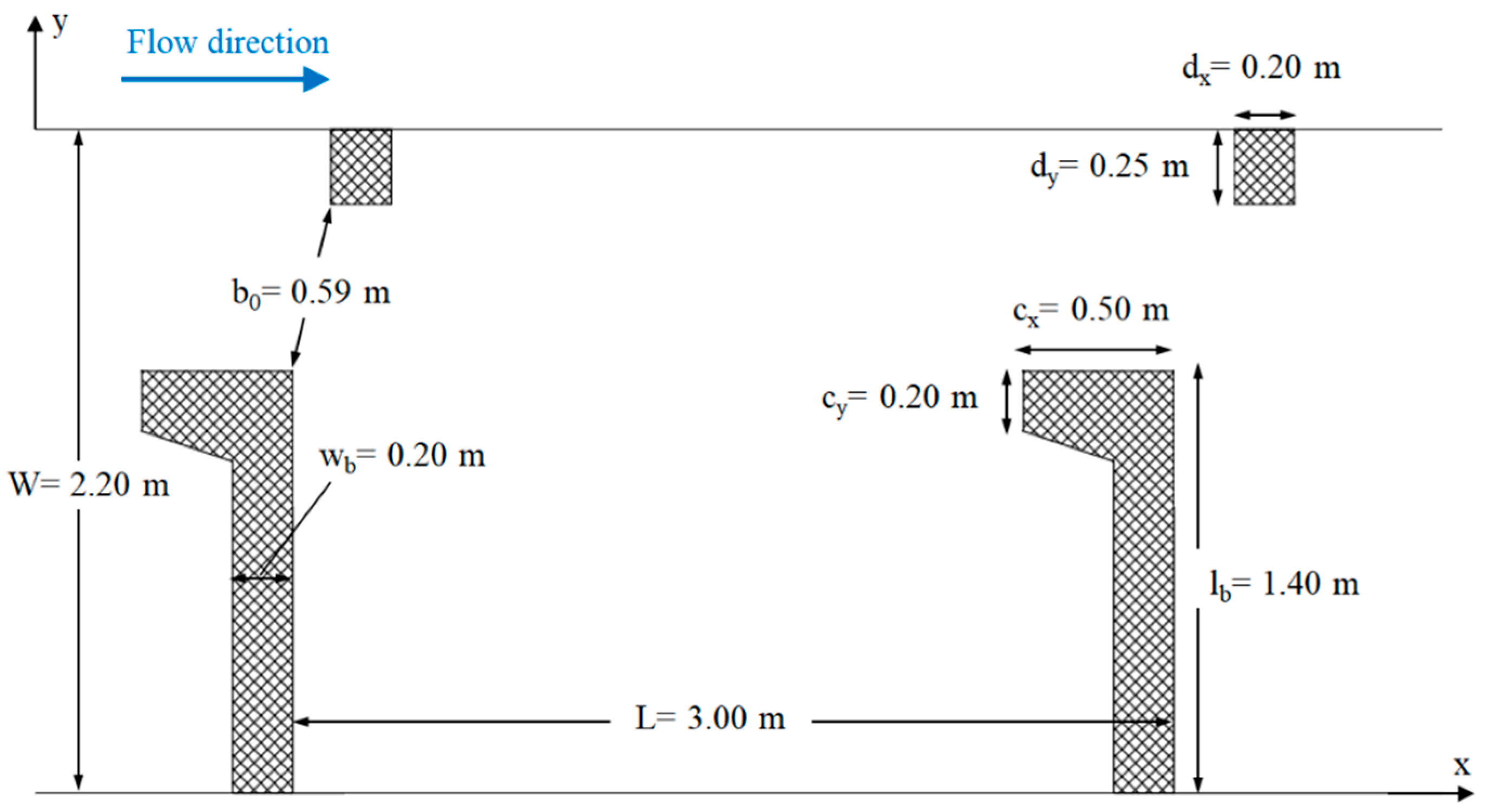
2.1. Geometrical Configuration

This study performed numerical simulations considering the existing field measurements at a vertical slot fishway (VSF) conducted by Bombač et al. [20], shown in Figure 1.

Measurements were obtained at the VSF situated at the Arto–Blanca HPP in Slovenia on river Sava. The prototype of the VSF considered in this study consists of two pools with the following dimensions: L = 3 m long and W = 2.2 m wide, having a vertical slot width of b₀ = 0.59 m and a slope of 1.67%. Field measurements were performed in steady-flow conditions, with a 1.0 m³/s discharge and an average water depth of 1.3 m (see Bombač, et al. [20] for more details). Several new VSF fishways were analyzed numerically to upgrade the reference design (Figure 2A1) to evaluate the enhancement of the hydraulic properties. Thus, We began by reducing in the pool width and setting to four values: W = 2 (10%), 1.85 (15%), 1.75 (20%) and 1.65m (25%) (Figure 2A2), considering five variants of angles between baffles, i.e., α = 0° (1dx width move to upstream), 12° (0.5dx width move to upstream), 20° (reference position), 30° (0.5dx width move to downstream), and 37° (1dx move to downstream) (Figure 2A3). The dx and dy are the width and length of a small baffle. In addition, another upgraded version of VSF by introducing cylindrical elements positioned after the opening behind the baffles was tested. Cylindrical elements consist of three different diameters, namely 0.3 (b₀/2), 0.15 (b₀/4), and 0.1 (b₀/6), with heights of 0.4 m invariants of the arrangement (Figure 2A4 and Figure 3).

2.2. Hydrodynamic Simulations

2.2.1. FLOW-3D^® Model

Numerical simulations were carried out using FLOW-3D, a well-known and established computational fluid dynamics software program. The treatment of the free surface is made the TruVOF (True Volume of Fluid) method based on the SOLA (SOLution Algorithm) algorithm developed by Hirt and Nichols [29].

Cells are represented by a cell fill variable (i.e., fraction function) value representing the ratio of the fluid volume to cell volume; the empty cells have a value of zero, whole cells a value of one, and cells that contain the free surface a value in the range 0–1. The water surface is then tracked in space and time as a first-order approximation according to the fluid-to-cell volume ratio and the location of the fluid in the surrounding cells. The TruVOF method considers only the fluid’s value, not the air’s; gas cells are considered empty. Previous studies used this method to reduce the time and graphically describe the free surface shape [30,31,32]. Moreover, the TruVOF method has also been transferred from a continuous approach, as used in this work, to a particle one, as reported in Abbasi et al. [29] and Di Francesco et al. [30].

2.2.2. Flow Equations

All features of the free-surface motions of the vertical slot fishway are simulated by the FLOW-3D commercial CFD code, as this software is equipped with a volume of fluid (VOF) scheme able to give a more realistic analysis of the free surface flow. Cartesian, staggered grids are employed to solve the RANS equations (Reynolds Average Navier–Stokes), composed by continuity and momentum equations:

$$\frac{\partial }{\partial x}(u{A}_x)+\frac{\partial }{\partial y}(v{A}_y)+\frac{\partial }{\partial z}(w{A}_z)=0$$

(1)

$$\frac{\partial U_i}{\partial t}+\frac{1}{V_F}\left(u_j{A}_j\frac{\partial u_i}{\partial x_j}\right)=-\frac{1}{\rho }\frac{\partial P}{\partial x_i}+G_i+f_i$$

(2)

where u, v, and w represent the components of velocity in x, y, and z-direction, V_F the volume fraction of fluid in each cell, A_x, A_y, and A_z the fractional areas open to flow in the subscript’s direction, ρ is the fluid density, P the hydrostatic pressure, G_i the gravitational acceleration in subscript direction and fi the Reynolds stress. The VOF transport equation is expressed:

$$\frac{\partial F}{\partial t}+\frac{1}{V_F}\left[\frac{\partial (F{A}_{x}u)}{\partial x}+\frac{\partial (F{A}_{y}v)}{\partial y}+\frac{\partial (F{A}_{z}w)}{\partial z}\right]=0$$

(3)

Here, F denotes the fraction function. In particular, as already stated, if a cell is empty F = 0, and if a cell is full F = 1 [33]. The free surface is determined at a position related to intermediate amounts of F (i.e., the user may usually determine F = 0.5, but another intermediate amount).

2.2.3. Turbulence Model

FLOW-3D^® has the capability of performing turbulence simulation using different models such as standard turbulence models, the k-ε turbulence model, and the RNG turbulence model. In this study, the RNG k-ε turbulence model estimates the shear stress near the wall. It has been proven to be sufficiently accurate; see Pourshahbaz, et al. [34] and Ghaderi, et al. [33], based on Yakhot and Orszag [35]. The RNG k-ε model can better deal with the high strain rate and the greater curvature of streamline flow. This model showed satisfactory outcomes in previous studies in complex geometry and flow fields on hydraulic structures such as spillways, culverts, and other hydraulic structures [31,33,36,37,38,39]. The RNG k-ε model is based on two equations; the first one (Equation (4)) expresses the energy in turbulence, called turbulent kinetic energy (TKE) (k), and the second one (Equation (5)) is the turbulent dissipation rate (ε), which determines the kinetic energy dissipation rate.

$$\frac{\partial (\rho k)}{\partial t}+\frac{\partial (\rho k{u}_i)}{\partial x_i}=\frac{\partial }{\partial x_j}[{\alpha }_k{\mu }_{eff}\frac{\partial k}{\partial x_j}]+G_k-G_B-\rho \epsilon -Y_M+S_k$$

(4)

$$\begin{array}{l}\frac{\partial (\rho \epsilon )}{\partial t}+\frac{\partial (\rho \epsilon u_i)}{\partial x_i}=\frac{\partial }{\partial x_j}[{\alpha }_{\epsilon }{\mu }_{eff}\frac{\partial \epsilon }{\partial x_j}]+C_{1\epsilon }\frac{\epsilon }{k}(G_k+C_{3\epsilon }{G}_b)-\\ C_{2\epsilon }^{}\rho \frac{{\epsilon }^2}{k}-R_{\epsilon }+S_{\epsilon }\end{array}$$

(5)

G_k is the generation of turbulent kinetic energy caused by the average velocity gradient. G_B is the generation of turbulent kinetic energy caused by buoyancy. S_k and S_ε are source terms. α_k and α_ε are inverse adequate Prandtl numbers for k and ε, respectively. μ_eff is the effective viscosity μ_eff = μ + μ_t. The μ_t is the eddy viscosity.

For the above equation:

$$R_{\epsilon }=\frac{C_{\mu }\rho {\eta }^3(1-\eta /{\eta }_0){\epsilon }^2}{k(1+\beta {\eta }^3)}$$

(6)

$${\mu }_t=\frac{\rho C_{\mu }{k}^2}{\epsilon }$$

(7)

The constant values for this model are [35]:

C_µ = 0.0845, C_1ε = 1.42, C_2ε = 1.68, C_3ε =1.0, σ_k = 0.7194, σ_ε = 0.7194, η₀ = 4.38, and β = 0.012.

Here, F denotes.

2.2.4. Numerical Domain

The geometry of the models is built represented through an STL (stereolithography) file. The numerical mesh is constructed to adopt two mesh blocks, a containing mesh block for the entire spatial domain and a nested block with refined cells for the area of interest. The small and large baffles occur. The fractional area volume obstacle representation (FAVOR) method generates grids.

In order to select an appropriate mesh structure and size essential for the accuracy and convergence of numerical solutions, the grid convergence index (GCI) is used to estimate the discretization error of several computational meshes. The analysis was developed following the Richardson extrapolation method [40]. Cell size was considered the minimum refinement ratio (r = G_coarse/Gf_ine), a value of 1.3, as Celik et al. [40] recommended. For this purpose, a refinement ratio of 1.34 was considered for reducing the grid sizes.

Table 1. Characteristics of the meshes tested in the convergence analysis.

Mesh	Nested Block Cell Size	Containing Block Cell Size	Number of Cell	Mesh
1	3 cm	4 cm	1,078,157	Coarse
2	2.85 cm	3.8 cm	1,689,598	Medium
3	2.6 cm	3.5 cm	2,268,478	Fine

shows some characteristics of the computational grids.

When testing the mesh convergence, the GCI values were computed using different mesh sizes. The analysis was based on the velocity component in two points (V1 and V2) in the longitudinal section located 0.50 m and 2 m downstream of the first baffle, giving GCI values in

Table 2. Grid convergence index (GCI) calculation.

Quantity	f3	f2	f1	p	GCI12	GCI23	Asymptotic Range
V1 (m/s)	1.09	1.21	1.36	3.11	0.55	0.62	0.9
V2 (m/s)	0.86	0.95	1.07	4	0.39	0.47	0.9

. Results of the CFD model were compared with the velocity measured at the same points, as shown in Figure 4. In this figure, S.1 to S.5 are sections from 1 to 5.

The apparent order of convergence p can be calculated as follows:

$$p=\ln \frac{(f_3-f_2)}{(f_2-f_1)}/\ln (r)$$

(8)

where f₁, f₂, f₃ are the parameters obtained from CFD simulations (f₁ corresponds to the fine mesh) and r is the refinement rate. Using the Richardson error estimator to compare the three grids, the fine-grid convergence index is defined as:

$$GC{I}_{fine}^{}=\frac{1.25\left|\epsilon \right|}{r_{}^p-1}$$

(9)

Here, ε = (f₂ − f₁)/f₁ is the approximate relative error between the medium and fine grids, respectively. Dimensionless indices GCI₁₂ and GCI₂₃ can be calculated as:

$$GC{I}_{12}^{}=\frac{1.25\left|\frac{f_2-f_1}{f_1}\right|}{r_{}^p-1}$$

(10)

Then, the grid independence is achieved. The parameters of the Grid Convergence Index (GCI) were calculated from Equation (8) through Equation (10) and are shown in Table 2.

Since the GCI values for the finer grid (GCI₁₂) are small if compared to the coarser one (GCI₂₃), it can be concluded that the aim of a grid-independent solution is reached, and no further mesh modification is necessary. Computed values of GCI₂₃/rpGCI₁₂ close to 1 indicate that the numerical solutions are within the asymptotic range of convergence. As a result, the selected mesh consists of a containing block with 3.5 cm cells and a nested block with 2.6 cm cells. (Figure 5).

Corresponding to the physical conditions of the problem, four different boundary conditions were considered. The inlet boundary condition was set as discharge flow rate (Q) with flow depth at the channel’s beginning. That specific discharge was subsequently used in this study. The outlet boundary condition (O) was selected as the outlet downstream of the VSF to prevent the downstream boundary effects on the last step results. No-slip conditions were applied at the wall boundaries and the bottom, assuming a law-of-the-wall velocity profile that modifies the wall shear stress magnitude. Atmospheric pressure (P) was employed at the top. Symmetry boundary condition (S) is also used at the inner boundaries. In the symmetry boundary condition, no shear stresses were calculated across the boundary [38]. Figure 6 shows the computational domain of the present study and associated boundary conditions. All analyses were continued until a steady-state was reached.

3. Results and Discussion

3.1. Model Validation

To verify the results obtained from the numerical modeling, the magnitude of the flow velocity, calculated V = |u, v| = (u² + v²)^0.5 from the numerical results is compared with the experimental data as shown in Figure 7. According to Figure 7, the results show that the trend and value obtained from numerical modeling satisfactorily agree with the experimental data.

Table 3. Calculated and measured values of the velocity magnitude in m/s for the reference model.

Location	x = 0.5 m		x = 1.0 m		x= 1.5 m		x = 2.0 m		x = 2.5 m
	Num	Exp	Num	Exp	Num	Exp	Num	Exp	Num	Exp
y = 0.9 m	0.085	0.156	0.121	0.142	0.155	0.138	0.149	0.120	0.149	0.310
y = 1.2 m	0.196	0.148	0.521	0.360	0.541	0.350	0.537	0.328	0.248	0.301
y = 1.5 m	1.401	1.263	1.421	1.212	1.214	1.043	1.114	0.954	1.164	0.946
y = 1.8 m	1.472	1.365	0.987	0.971	1.131	1.051	1.113	1.091	1.124	1.150
y = 2.1 m	0.179	0.205	0.070	0.059	0.213	0.32	0.389	0.661	0.638	0.891
Mean Error (%)	6.20		10.4		9.74		4.61		5.67

summarizes the velocity magnitude values in some vertical distance for calculated and measured data.

From Table 3, the most significant differences between the calculated and measured values occur in the middle of the baffles, where the flow is significantly more complex than in other parts of the structure. The overall maximum error is 10.4%, which corroborates the ability of the numerical model to reproduce the main characteristics of a VSF.

3.2. The Flow Pattern of Vertical Slot Fishway

The pool flow creates three distinct zones that vary in position and volume depending on the fish pass slope, baffles geometry, and the pool width: a jet from the slot that traverses the pool with decreasing velocity and two separate recirculation zones on each side of the jet [41]. The recirculation around an axis perpendicular to the channel bed dissipates the jet’s energy in each pool.

The main flow from the slot comes into the pools as a curved jet that opens before converging towards the next slot (Figure 8). The jet originates a large recirculation zone, occupying about half of the pool, showing an unsteady flow around the large baffle, affecting the fish swimming performance [20,42]. The kinetic energy of the velocity fluctuations is represented by the turbulent kinetic energy (TKE); in other words, TKE represents the mean kinetic energy per unit mass associated with eddies in turbulent flow conditions. Considering the continuous values of velocities in the flow direction (u₁, u₂, u₃, …, u_n), the value of the root mean square velocity, u_rms, is obtained as:

$$u_{rms}=\sqrt{1/n(u_1^2+u_2^2+u_3^2+\dots +u_n^2)}$$

(11)

Then, TKE is calculated as:

$$TKE=\frac{1}{2}\left(u_{rms}^2+v_{rms}^2+w_{rms}^2\right)$$

(12)

The levels of turbulent kinetic energy are categorized as “low” for k ≤ 0.05 J/kg and “high” for k > 0.05 J/kg [10,41]. In fishways, fishes prefer the areas with “low” turbulent kinetic energy levels rather than those with “high” levels [21,43]. Indeed, turbulence and eddies have a stronger influence mainly on the swimming performance of larger fish [21]. TKE distribution presented in Figure 9 shows that maximum values of TKE are observed downstream of the slot entrance. Away from the jet area, kinetic energy then dissipated rapidly as jet velocity decays as it traveled through the rest of the pool. Figure 9 shows the distribution of ε and k, highlighting their similar pattern. In the most significant portion of the pool, the maximum ε values are encountered in the incoming jet.

According to Figure 10, two areas downstream of the large and short baffles have high turbulent kinetic energy. The intensity of TKE downstream of the short baffle is greater than that of the large type. As jet velocity moves away from the baffles, the intensity of the turbulent kinetic energy decreases.

3.3. Influence of Angle between Baffles on V_max and TKE in the Slot

The maximum velocity of the flow is one of the most critical hydraulic parameters of VSF design: it has to be smaller than the speed of the weakest fish that migrates in the pool [21,42,43]. The jet’s velocity entering the slots has the highest value between the two baffles (Figure 11). Figure 12 shows the maximum velocity of the flow at x = 0.5 m downstream of the baffles for all models.

From Figure 12, it is evident that the value of maximum velocity is greater for a smaller angle (α = 0°) and decreases as the angle between baffles increases. A larger angle between baffles changes the direction of the flow-through of the pool between larger baffles, causing the recirculation zone between larger baffles to decrease, while the recirculation zone between smaller baffles increases (Figure 13).

As shown in Figure 13, increasing the angle results in greater turbulent kinetic energy and, thus, smaller velocities between larger baffles. This effect is much smaller at smaller angles. The kinetic energy is transported to the next slot almost without dissipation. Figure 14 illustrates the maximum TKE values for VSF with various angles between baffles at x = 0.5 m and x = 2 m. The results show that the maximum TKE values occur for the larger angles. Increasing the angle between baffles results in an average 26% increase of maximum TKE compared to the reference position; in contrast, the highest reduction of maximum TKE reached nearly 20% at the smallest angle (α = 0°).

3.4. Influence of the Pool Width on V_max and TKE

The mainstream pattern at the maximum width of the pool enters the pool from the upstream slot as a curved jet and is transferred to the next slot. The flow jet creates a large recirculation zone with unstable movement around the large baffles. When the width of the pool is decreased, and, correspondingly, the maximum velocity of the jet is increased, the impact of the jet at the opposite wall becomes much less noticeable. As a result, the intensity of the circulation zone between the two large baffles is reduced (Figure 15). With decreasing the width of the pool, the recirculation shapes and the location of their centers did not change much, irrespective of the intensity. At the same time, velocities remained identical overall in the pool, from the channel bed to the free surface. Except in the slot zone, the maximum velocity was highly more significant than the reference width of the pool (i.e., W = 2.2 m).

In Figure 16, the maximum velocity of the flow at x = 0.5 m and x = 2.5 m downstream of the baffles is shown for all models. The velocities in the mainstream flow through the slots are high. However, in the areas behind large baffles, the flow velocity values are low as the width of the pool decreases, the maximum velocity of the principal flow increases. A 25 % reduction in pool width increases the maximum velocity of the flow by an average of 21.5 %. The increase of the flow velocity may influence the attractiveness of the large-size of fish to the entrance of the fish pass positively; nevertheless, it may not have the same effect on the small-size of fish [15,43].

Figure 17 shows the turbulent kinetic energy (TKE) for different pool widths. The maximum values are attained in the jet and on the edge of recirculation zones. The location and volume of zones where TKE remains high vary with width. The volume of zones with low values of turbulent energy increased considerably with pool width.

Only the zone downstream of the small baffle remains the same, in agreement with previous research conducted by Wu, et al. [44]; the pool width (i.e., the pool volume) influences turbulent kinetic energy, whereas the flow discharge has little or no influence. From Figure 18, the average turbulent kinetic energy values, for reduced width I = 10%, 15%, 20% and 25%, were 0.0686 J/kg, 0.0675 J/kg, 0.068 J/kg, and 0.069 J/kg, respectively. A 25% reduction in pool width increases the maximum velocity of the flow by an average of 3.5%.

Although flow rate has little or no influence on the TKE, its quantity and variability are essential for ensuring the high efficiency of the fishways. In addition, the flow rate (e-flows) released in the fishway should be defined, considering the fish species requirements and their life stages [2,4,16,42,45].

3.5. Influence of the Cylinder’s Adjunction on V_max and TKE

An obstacle cylinder of diameter equal to half of the slot width b₀/2, placed after the opening behind the baffles (C1). Other cylinders with different diameters and arrangements were placed in the periphery of the larger diameter inside the pool (Figure 19C2–C6). Figure 19 illustrates the velocity streamlines for fishway models with cylinders inside the pool and in different arrangements. The results show that the jet from the slot widened in the pool before converging towards the following slot. For an obstacle located in the jet in the middle of the pool, the principal flow, of width higher than the geometry diameter, turned around the obstacle on each side. The diameter and arrangement of the cylinder modified the flow pattern. For example, the cylinders of type C6 reduces the vortices in the recirculation zone.

In contrast, the location of cylinder C3 intensifies the vortex. The maximum velocity of the principal flow is reduced in an obstacle cylinder inside the pool. This can be due to the jet impacting the face of the cylinder or passing it through small cylinders. The maximum velocity of the flow corresponding to x = 0.5 m and x = 2.5 m downstream of the baffles is shown in Figure 20.

The use of cylinders with a smaller diameter and arrangement types, namely C3, C4, and C6, further reduces the principal flow velocity inside the pool. Overall, the maximum velocity of the flow decreased by an average of 16.5 %. The dimension of the recirculation depended on the configuration and arrangement of the cylinder. When the jets impacted the cylinder with a larger diameter (C1), the two principal flows were diverted from the cylinder, near the walls with very curved trajectories. In this case, the reattachment point took place far downstream from the cylinder, and the impact of the jet at the opposite wall became much noticeable; the recirculation behind the cylinder was more significant. On the contrary, when cylinders with smaller diameters are used, the principal flows are less curved. The volume of zones with low values of turbulent energy increased considerably with smaller diameters of cylinders (Figure 21).

Figure 22 shows the maximum turbulent kinetic energy (TKE) for various cylinders arrangement. Due to the collision of the principal flow with the cylinders, the turbulent kinetic energy values inside the pool increase. Models C1 and C4 further increased the amount of TKE by 14.5% and 13%, respectively. Models C1, C2, and C6 induced the lowest increase of the TKE.

4. Conclusions

Fish-friendly flow conditions are crucial in ensuring effective fishway functioning. The results presented in this study underlines the importance of the geometric configuration in ensuring the high functionality of vertical slot fishway. After numerical investigation of the different configurations of VSF, the following major conclusions can be drawn:

Smaller angles between baffles increase the V_max and decrease the maximum turbulent kinetic energy (TKE_max); the opposite result was obtained when increasing angles between baffles. Namely, the V_max was increased up to 17.9% for α = 0° and decreased up to 20.37% for α = 37°; in contrast, TKE_max decreased up to −20% for α = 0° and increased up to 26.5% for α = 37°.

Narrowing the pool width increased the V_max linearly; nevertheless, narrowing the pool width did not significantly affect the TKE_max as the maximum difference was only +3.5%. Using cylinders with a large diameter decreased the V_max and increased TKE_max; in contrast, using cylinders with smaller diameters further reduces the V_max velocity inside the pool while increasing the TKE_max. In the case of cylinders, in addition to the diameter, the configuration and arrangement of the cylinder within the pool have a significant influence on the V_max and TKE_max variation. In that regard, the C6 model demonstrated the best performance, especially regarding the flow regime and principal flow velocity inside the pool. Overall, the maximum velocity was reached at near 77% of the water depth in all cases.

Although this study serves as a reliable reference for better design and upgrading the traditional design of VSF with a more sustainable and practical configuration, the numerical investigation could be more robust if verified with the experimental investigation. Thus, future research should involve testing the proposed VSF configurations in this study experimentally and/or on the field; nevertheless, the latter is not very common as it is costly. In addition, to refine the configuration of the VSF, the experimental work should not involve investigating only the hydraulic properties but also fish swimming behavior and performance considering different fish species and life stages. Finally, the findings resulted from this study serve as a guideline for hydraulic engineers to construct better fishways in order to enable longitudinal connectivity and support the sustainable development of hydraulic structures, such as hydropower plants.

References

1. Chen, S.; Chen, B.; Fath, B.D. Assessing the cumulative environmental impact of hydropower construction on river systems based on energy network model. Renew. Sustain. Energy Rev. 2015, 42, 78–92. [Google Scholar] [CrossRef]
2. Kuriqi, A.; Pinheiro, A.N.; Sordo-Ward, A.; Garrote, L. Influence of hydrologically based environmental flow methods on flow alteration and energy production in a run-of-river hydropower plant. J. Clean. Prod. 2019, 232, 1028–1042. [Google Scholar] [CrossRef]
3. Botelho, A.; Ferreira, P.; Lima, F.; Pinto, L.M.C.; Sousa, S. Assessment of the environmental impacts associated with hydropower. Renew. Sustain. Energy Rev. 2017, 70, 896–904. [Google Scholar] [CrossRef]
4. Kuriqi, A.; Pinheiro, A.N.; Sordo-Ward, A.; Bejarano, M.D.; Garrote, L. Ecological impacts of run-of-river hydropower plants—Current status and future prospects on the brink of energy transition. Renew. Sustain. Energy Rev. 2021, 142, 110833. [Google Scholar] [CrossRef]
5. Benejam, L.; Saura-Mas, S.; Bardina, M.; Solà, C.; Munné, A.; García-Berthou, E. Ecological impacts of small hydropower plants on headwater stream fish: From individual to community effects. Ecol. Freshw. Fish 2016, 25, 295–306. [Google Scholar] [CrossRef]
6. Zarfl, C.; Berlekamp, J.; He, F.; Jähnig, S.C.; Darwall, W.; Tockner, K. Future large hydropower dams impact global freshwater megafauna. Sci. Rep. 2019, 9, 18531. [Google Scholar] [CrossRef] [PubMed] [Green Version]
7. Couto, T.B.A.; Messager, M.L.; Olden, J.D. Safeguarding migratory fish via strategic planning of future small hydropower in Brazil. Nat. Sustain. 2021, 4, 409–416. [Google Scholar] [CrossRef]
8. Datry, T.; Boulton, A.J.; Bonada, N.; Fritz, K.; Leigh, C.; Sauquet, E.; Tockner, K.; Hugueny, B.; Dahm, C.N. Flow intermittence and ecosystem services in rivers of the Anthropocene. J. Appl. Ecol. 2018, 55, 353–364. [Google Scholar] [CrossRef] [PubMed] [Green Version]
9. Pfister, S.; Saner, D.; Koehler, A. The environmental relevance of freshwater consumption in global power production. Int. J. Life Cycle Assess. 2011, 16, 580–591. [Google Scholar] [CrossRef] [Green Version]
10. Santos, J.M.; Silva, A.; Katopodis, C.; Pinheiro, P.; Pinheiro, A.; Bochechas, J.; Ferreira, M.T. Ecohydraulics of pool-type fishways: Getting past the barriers. Ecol. Eng. 2012, 48, 38–50. [Google Scholar] [CrossRef]
11. Branco, P.; Santos, J.M.; Katopodis, C.; Pinheiro, A.; Ferreira, M.T. Pool-Type Fishways: Two Different Morpho-Ecological Cyprinid Species Facing Plunging and Streaming Flows. PLoS ONE 2013, 8, e65089. [Google Scholar] [CrossRef]
12. Silva, A.; Santos, J.; Ferreira, M.; Pinheiro, A.; Katopodis, C. Passage efficiency of offset and straight orifices for upstream movements of Iberian barbel in a pool-type fishway. River Res. Appl. 2012, 28, 529–542. [Google Scholar] [CrossRef]
13. Romão, F.; Quaresma, A.L.; Santos, J.M.; Amaral, S.D.; Branco, P.; Pinheiro, A.N. Multislot Fishway Improves Entrance Performance and Fish Transit Time over Vertical Slots. Water 2021, 13, 275. [Google Scholar] [CrossRef]
14. Romão, F.; Quaresma, A.L.; Santos, J.M.; Branco, P.; Pinheiro, A.N. Cyprinid passage performance in an experimental multislot fishway across distinct seasons. Mar. Freshw. Res. 2019, 70, 881–890. [Google Scholar] [CrossRef]
15. Katopodis, C. Introduction to Fishway Design; Freshwater Institute, Central and Arctic Region, Department of Fisheries and Oceans: Winnipeg, MB, Canada, 1992. [Google Scholar]
16. Kuriqi, A.; Pinheiro, A.N.; Sordo-Ward, A.; Garrote, L. Water-energy-ecosystem nexus: Balancing competing interests at a run-of-river hydropower plant coupling a hydrologic–ecohydraulic approach. Energy Convers. Manag. 2020, 223, 113267. [Google Scholar] [CrossRef]
17. Clay, C.H.; Eng, P. Design of Fishways and Other Fish Facilities; CRC Press: Boca Raton, FL, USA, 2017. [Google Scholar]
18. Larinier, M.; Travade, F.; Porcher, J.P. Fishways: Biological basis, design criteria and monitoring. Bull. Français Pêche Piscic. 2002, 634, 208. [Google Scholar]
19. Silva, A.T.; Lucas, M.C.; Castro-Santos, T.; Katopodis, C.; Baumgartner, L.J.; Thiem, J.D.; Aarestrup, K.; Pompeu, P.S.; O’Brien, G.C.; Braun, D.C. The future of fish passage science, engineering, and practice. Fish Fish. 2018, 19, 340–362. [Google Scholar] [CrossRef] [Green Version]
20. Bombač, M.; Novak, G.; Mlačnik, J.; Četina, M. Extensive field measurements of flow in vertical slot fishway as data for validation of numerical simulations. Ecol. Eng. 2015, 84, 476–484. [Google Scholar] [CrossRef]
21. Silva, A.T.; Katopodis, C.; Santos, J.M.; Ferreira, M.T.; Pinheiro, A.N. Cyprinid swimming behaviour in response to turbulent flow. Ecol. Eng. 2012, 44, 314–328. [Google Scholar] [CrossRef] [Green Version]
22. Bombač, M.; Četina, M.; Novak, G. Study on flow characteristics in vertical slot fishways regarding slot layout optimization. Ecol. Eng. 2017, 107, 126–136. [Google Scholar] [CrossRef]
23. Abbasi, S.; Fatemi, S.; Ghaderi, A.; Di Francesco, S. The Effect of Geometric Parameters of the Antivortex on a Triangular Labyrinth Side Weir. Water 2021, 13, 14. [Google Scholar] [CrossRef]
24. Tarrade, L.; Texier, A.; David, L.; Larinier, M. Topologies and measurements of turbulent flow in vertical slot fishways. Hydrobiologia 2008, 609, 177. [Google Scholar] [CrossRef] [Green Version]
25. Hameed, I.H.; Hilo, A.N. Numerical Analysis on the Effect of Slot Width on the Design of Vertical Slot Fishways. In Proceedings of IOP Conference Series: Materials Science and Engineering; IOP Publishing: Bristol, UK, 2021; Volume 1090, p. 012094. [Google Scholar]
26. Cea, L.; Pena, L.; Puertas, J.; Vázquez-Cendón, M.; Peña, E. Application of several depth-averaged turbulence models to simulate flow in vertical slot fishways. J. Hydraul. Eng. 2007, 133, 160–172. [Google Scholar] [CrossRef]
27. Bravo-Córdoba, F.J.; Fuentes-Pérez, J.F.; Valbuena-Castro, J.; Martínez de Azagra-Paredes, A.; Sanz-Ronda, F.J. Turning Pools in Stepped Fishways: Biological Assessment via Fish Response and CFD Models. Water 2021, 13, 1186. [Google Scholar] [CrossRef]
28. Li, G.; Sun, S.; Liu, H.; Zheng, T. Schizothorax prenanti swimming behavior in response to different flow patterns in vertical slot fishways with different slot positions. Sci. Total Environ. 2021, 754, 142142. [Google Scholar] [CrossRef] [PubMed]
29. Hirt, C.W.; Nichols, B.D. Volume of fluid (VOF) method for the dynamics of free boundaries. J. Comput. Phys. 1981, 39, 201–225. [Google Scholar] [CrossRef]
30. Ghaderi, A.; Abbasi, S. Experimental and Numerical Study of the Effects of Geometric Appendance Elements on Energy Dissipation over Stepped Spillway. Water 2021, 13, 957. [Google Scholar] [CrossRef]
31. Daneshfaraz, R.; Ghaderi, A.; Sattariyan, M.; Alinejad, B.; Asl, M.M.; Di Francesco, S. Investigation of Local Scouring around Hydrodynamic and Circular Pile Groups under the Influence of River Material Harvesting Pits. Water 2021, 13, 2192. [Google Scholar] [CrossRef]
32. Di Francesco, S.; Biscarini, C.; Manciola, P. Numerical simulation of water free-surface flows through a front-tracking lattice Boltzmann approach. J. Hydroinform. 2014, 17, 1–6. [Google Scholar] [CrossRef]
33. Ghaderi, A.; Dasineh, M.; Aristodemo, F.; Aricò, C. Numerical Simulations of the Flow Field of a Submerged Hydraulic Jump over Triangular Macroroughnesses. Water 2021, 13, 674. [Google Scholar] [CrossRef]
34. Pourshahbaz, H.; Abbasi, S.; Pandey, M.; Pu, J.H.; Taghvaei, P.; Tofangdar, N. Morphology and hydrodynamics numerical simulation around groynes. ISH J. Hydraul. Eng. 2020, 1–9. [Google Scholar] [CrossRef]
35. Yakhot, V.; Orszag, S.A. Renormalization group analysis of turbulence. I. Basic theory. J. Sci. Comput. 1986, 1, 3–51. [Google Scholar] [CrossRef]
36. Ghaderi, A.; Dasineh, M.; Aristodemo, F.; Ghahramanzadeh, A. Characteristics of free and submerged hydraulic jumps over different macroroughnesses. J. Hydroinf. 2020, 22, 1554–1572. [Google Scholar] [CrossRef]
37. Daneshfaraz, R.; Ghaderi, A.; Akhtari, A.; Di Francesco, S. On the Effect of Block Roughness in Ogee Spillways with Flip Buckets. Fluids 2020, 5, 182. [Google Scholar] [CrossRef]
38. Ghaderi, A.; Abbasi, S.; Di Francesco, S. Numerical Study on the Hydraulic Properties of Flow over Different Pooled Stepped Spillways. Water 2021, 13, 710. [Google Scholar] [CrossRef]
39. Ran, D.; Wang, W.; Hu, X. Three-dimensional numerical simulation of flow in trapezoidal cutthroat flumes based on FLOW-3D. Front. Agric. Sci. Eng. 2018, 5, 168–176. [Google Scholar] [CrossRef] [Green Version]
40. Celik, I.B.; Ghia, U.; Roache, P.J.; Freitas, C. Procedure for estimation and reporting of uncertainty due to discretization in CFD applications. J. Fluids Eng.-Trans. ASME 2008, 130, 078001. [Google Scholar]
41. Marriner, B.A.; Baki, A.B.M.; Zhu, D.Z.; Cooke, S.J.; Katopodis, C. The hydraulics of a vertical slot fishway: A case study on the multi-species Vianney-Legendre fishway in Quebec, Canada. Ecol. Eng. 2016, 90, 190–202. [Google Scholar] [CrossRef]
42. Quaresma, A.L.; Pinheiro, A.N. Modelling of Pool-Type Fishways Flows: Efficiency and Scale Effects Assessment. Water 2021, 13, 851. [Google Scholar] [CrossRef]
43. Li, Y.; Wang, X.; Xuan, G.; Liang, D. Effect of parameters of pool geometry on flow characteristics in low slope vertical slot fishways. J. Hydraul. Res. 2020, 58, 395–407. [Google Scholar] [CrossRef]
44. Wu, S.; Rajaratnam, N.; Katopodis, C. Structure of flow in vertical slot fishway. J. Hydraul. Eng. 1999, 125, 351–360. [Google Scholar] [CrossRef]
45. Kuriqi, A.; Pinheiro, A.N.; Sordo-Ward, A.; Garrote, L. Flow regime aspects in determining environmental flows and maximising energy production at run-of-river hydropower plants. Appl. Energy 2019, 256, 113980. [Google Scholar] [CrossRef]
Figure 1. VSF Blanca’s prototype geometry and slot and pool details after Bombač, et al. [20].
Water 13 02711 g001
Figure 2. Plan views of fishway pools: (A1) Reference; (A2) reducing pool width; (A3) with variants of angles between baffles and (A4) with cylinders.
Water 13 02711 g002
Figure 3. Cylinders details and positions used in the reference VSF.
Water 13 02711 g003aWater 13 02711 g003b
Figure 4. Cross-sections right to the longitudinal axis of the fishway used for results analysis.
Water 13 02711 g004
Figure 5. Sketch of mesh set-up.
Water 13 02711 g005
Figure 6. The considered boundary conditions on the numerical domain in FLOW-3D.
Water 13 02711 g006
Figure 7. Velocity magnitude against vertical distance at different x locations.
Water 13 02711 g007aWater 13 02711 g007b
Figure 8. Mean flow velocity pattern inside the pool of the reference VSF.
Water 13 02711 g008
Figure 9. Turbulent kinetic energy and dissipation rate at a mid-depth horizontal plane for the reference VSF: (a) k (j/kg); (b) ε (j/kg/s).
Water 13 02711 g009
Figure 10. Turbulent kinetic energy for vertical distance at different x locations.
Water 13 02711 g010
Figure 11. Streamlines of velocity for reference VSF (α = 20°) and VSF with various angles between baffles.
Water 13 02711 g011aWater 13 02711 g011b
Figure 12. Velocity magnitude and maximum velocity of the flow and various angles at x = 0.5 m.
Water 13 02711 g012
Figure 13. Contours of turbulent kinetic energy (J/kg) for reference VSF (α = 20°) and VSF with various angles between baffles.
Water 13 02711 g013aWater 13 02711 g013b
Figure 14. Maximum turbulent kinetic energy for the reference VSF and the VSF with various angles between baffles at three cross-sections.
Water 13 02711 g014
Figure 15. Streamlines of velocity for reference VSF and VSF with various widths of the pool.
Water 13 02711 g015
Figure 16. Velocity magnitude and maximum velocity of the flow and width of the pool.
Water 13 02711 g016
Figure 17. Contours of turbulent kinetic energy (J/kg) for the reference VSF and the VSF with various pool widths.
Water 13 02711 g017
Figure 18. Maximum turbulent kinetic energy for the reference VSF and the VSF various pool widths at three cross-sections.
Water 13 02711 g018
Figure 19. Streamlines of velocity for reference VSF and VSF with various cylinders arrangement.
Water 13 02711 g019
Figure 20. Velocity magnitude and maximum flow velocity for the reference VSF and the VSF with various cylinders arrangement.
Water 13 02711 g020
Figure 21. Contours of turbulent kinetic energy (J/kg) for reference VSF and VSF with various cylinders arrangement.
Water 13 02711 g021
Figure 22. Maximum turbulent kinetic energy for the reference VSF and the VSF with various cylinders arrangement.
Water 13 02711 g022