Assessing the Impact of Soil Moisture on Canopy Transpiration Using a Modified Jarvis-Stewart Model

Abstract

In dryland regions, soil moisture is an important limiting factor for canopy transpiration (T). Thus, clarifying the impact of soil moisture on T is critical for comprehensive forest—water management and sustainable development. In this study, T, meteorological factors (reference evapotranspiration, ET_ref), soil moisture (relative soil water content, RSWC), and leaf area index (LAI) in a Larix principis-rupprechtii plantation of Liupan Mountains in the dryland region of Northwest China were simultaneously monitored during the growing seasons in 2017–2019. A modified Jarvis—Stewart model was established by introducing the impact of RSWC in different soil layers (0–20, 20–40, and 40–60 cm, respectively) to quantify the independent contribution of RSWC of different soil layers to T. Results showed that with rising ET_ref, T firstly increased and then decreased, and with rising RSWC and LAI, T firstly increased and then gradually stabilised, respectively. The modified Jarvis—Stewart model was able to give comparable estimates of T to those derived from sap flow measurements. The contribution of RSWC to T in different soil layers has obvious specificity, and the contribution rate of 20–40 cm (13.4%) and 0–20 cm soil layers (6.6%) where roots are mainly distributed is significantly higher than that of 40–60 cm soil layer (1.9%). As the soil moisture status changes from moist (RSWC_0–60cm ≥ 0.4) to drought (RSWC_0–60cm < 0.4), the role of the soil moisture in the 0–20 cm soil layer increased compared with other layers. The impacts of soil moisture that were coupled into the Jarvis—Stewart model can genuinely reflect the environmental influence and can be used to quantify the contributions of soil moisture to T. Thus, it has the potential to become a new tool to guide the protection and management of forest water resources.

1. Introduction

As the main component of evapotranspiration, canopy transpiration (T) accounts for 50–90% of the forest evapotranspiration [1,2], and plays a vital role in regional water supplies. In recent decades, the continuous warming and drying phenomenon in the Loess Plateau has created a water resource problem that has become increasingly prominent in Northwest China [3]. The temperature in the Loess Plateau has increased by 1.91 °C and since 1961 the annual precipitation has decreased by 29.1 mm due to warming [4]. Furthermore, the large-scale afforestation plan in the 1980s caused severe forest water conflicts while causing soil and water conservation [5,6]. Many artificial forests in the planned area grew abnormally and could not form canopy closures. This is because soil drought has deteriorated the ecological environment in some areas [7], causing water loss and senescence of plant leaves and accelerated shedding [8]. In turn, excessive loss of leaf volume limits the photosynthetic and transpiration area of plants, which eventually leads to abnormal growth [9]. Therefore, accurately simulating canopy T and quantifying the effects of soil moisture in a complex environment could significant help coordinate forest-water conflicts and water resource management.

The response of T to environmental changes involves complex mechanisms [10], but generally, the environmental control of T can be simplified to three aspects: the self—determined canopy water delivery capacity [11], the atmospheric driving force [11,12,13], and the soil water supply capacity [14,15]. Among these aspects, the canopy water delivery capacity is regarded as an intrinsic factor determined by the canopy leaves [16], which can be characterized by the leaf area index (LAI). Many studies have shown that T is closely related to LAI, and have found a linear [17] or saturated growth exponential relationship between the two [11,18]. Research by Wang et al. [7] found that severe atmospheric conditions (such as intense light competition) would decline the response threshold of T to the LAI. It is thus imperative to accurately describe the climatic conditions during the study period. Meteorological conditions are determinants of transpiration and many current studies use multiple meteorological factors to reflect the driving force of the atmosphere on T [15,19,20,21]. However, due to the extensive correlations between these meteorological factors, it is difficult to accurately reflect the comprehensive impacts of the atmosphere on T. Several studies have shown that as a composite index characterising local meteorological conditions and evaporation capacity, reference evapotranspiration, (ET_ref) can effectively reflect the driving force of the atmosphere on T [10,18]. Wu et al. [22] found that ET_ref explained more than 60% of the T variation of Robinia pseudoacacia plantation on the Loess Plateau in China. In coniferous forests of southern France, ET_ref reportedly linearly correlates with T in the range of 0–7 mm d⁻¹ [23]. This shows a close relationship between ET_ref and T. Different from the ET_ref and LAI, the influence of the soil water supply capacity on T is usually reflected in limitations to T due to water stress [24]. Studies in the semi-humid regions of Northwest China have shown that when RSWC is less than 0.38, coniferous forests will be under drought stress and the restriction of RSWC will result in losses in T of up to 11.6% [7,25]. Previous investigations also indicated that canopy T was affected by the coupling of leaves, atmosphere, and soil moisture; thus, ET_ref, RSWC, and LAI should be included when investigating the T response mechanisms.

In natural conditions, T is mainly affected by the interactions of ET_ref, RSWC, and LAI. Several studies have been conducted on the comprehensive influence of multiple factors on T. For example, Li et al. [26] modelled the comprehensive impact of soil moisture and atmospheric conditions based on a modified Jarvis-Stewart model driven by soil moisture and potential evaporation, Whitley et al. [27] introduced LAI to Jarvis—Stewart model and optimised its performance during years characterised by large fluctuations in leaf volume. However, these studies did not consider the impact of soil moisture across the soil profile and their levels on T. In a study of Pinus sylvestris forest by Llorens et al. [28], it was found that the soil moisture in different soil layers had a noticeable effect on T. Studies by Ehleringer et al. [29] and Flanaganin et al. [30] in the desert ecosystems of the southern United States found that deep-rooted plants mainly used deep soil moisture and groundwater during drought conditions. In contrast, plants with developed lateral roots relied on shallow soil moisture for replenishment, reflecting the differences in the effects of soil moisture in different soil layers on T. Liu et al. [16] also suggested that it is better to add the impact of soil moisture in different soil layers into the T model to accurately evaluate T. The current study however has not continuously quantified the dynamic contributions of the different soil layers in relation to T. Liu et al. [31] used the stable isotope approach to quantify different water source, and found that by gradually moistening the soil, the contribution of the deep soil water by Quercus variabilis increased from 22.8% to 26.9%, and the shallow soil water decreased from 20.0% to 10.7% in the rocky mountainous area of North China. However, the stable isotope method is costly and cannot continuously obtain changes in the relative contribution rates of the different soil layers; there are limitations in understanding the water absorption strategies of the plants under the different soil moisture conditions. Consequently, developing or improving a more comprehensive model to reflect the influence of soil moisture in different soil layers on T and developing a new method based on the model to quantify its dynamic contributions to T is critical.

Larix principis-rupprechtii is a drought-tolerant tree species and is widely used for afforestation in dryland areas in North China due to its unique physiological characteristics such as small leaf size, thick leaf cuticle layers, and developed root system. This because smaller leaves can effectively prevent heat accumulation from causing excessive temperature stress in the leaf boundary layer and causing water loss [32]; thick cuticle layers are more conducive to maintaining water in drought conditions [33], and the developed root system allows plants to adjust their water use strategies as drought intensifies [34]. With high resistance to drought, L. principis-rupprechtii has become the main afforestation tree species in the Liupan Mountain area of Northwest China and plays an important role in water storage and soil conservation in the region. However, the precipitation distribution in this area is uneven, and the seasonal variation of soil moisture is evident. How the T of larch responds to the variations of drying and wetting alternation of soil moisture in different soil layers on T was unclear. Therefore, this study attempts to reveal how the T of Larix principis-rupprechtii plantation responds to the variation in soil water content and determine the contribution of soil water content to T under different soil moisture conditions. This study aimed to develop a forest T model to quantify the continuous influence of soil moisture levels in different soil layers and different moisture condition (moist or drought) on T. To achieve this, field observations, including canopy transpiration, meteorological factors, soil moisture, and LAI in an L. principis-rupprechtii plantation during the 2017–2019 growing season (May–September) was conducted. The objectives of this study were: (1) to determine the response relationship of T to ET_ref, RSWC in different soil layers, and LAI; (2) to improve the Jarvis-Stewart model which can reflect the impact of soil moisture in different soil layers; and (3) to quantify the independent contributions of RSWC in different soil layer on T across different years and soil moisture conditions based on the modified Jarvis-Stewart model.

2. Materials and Methods

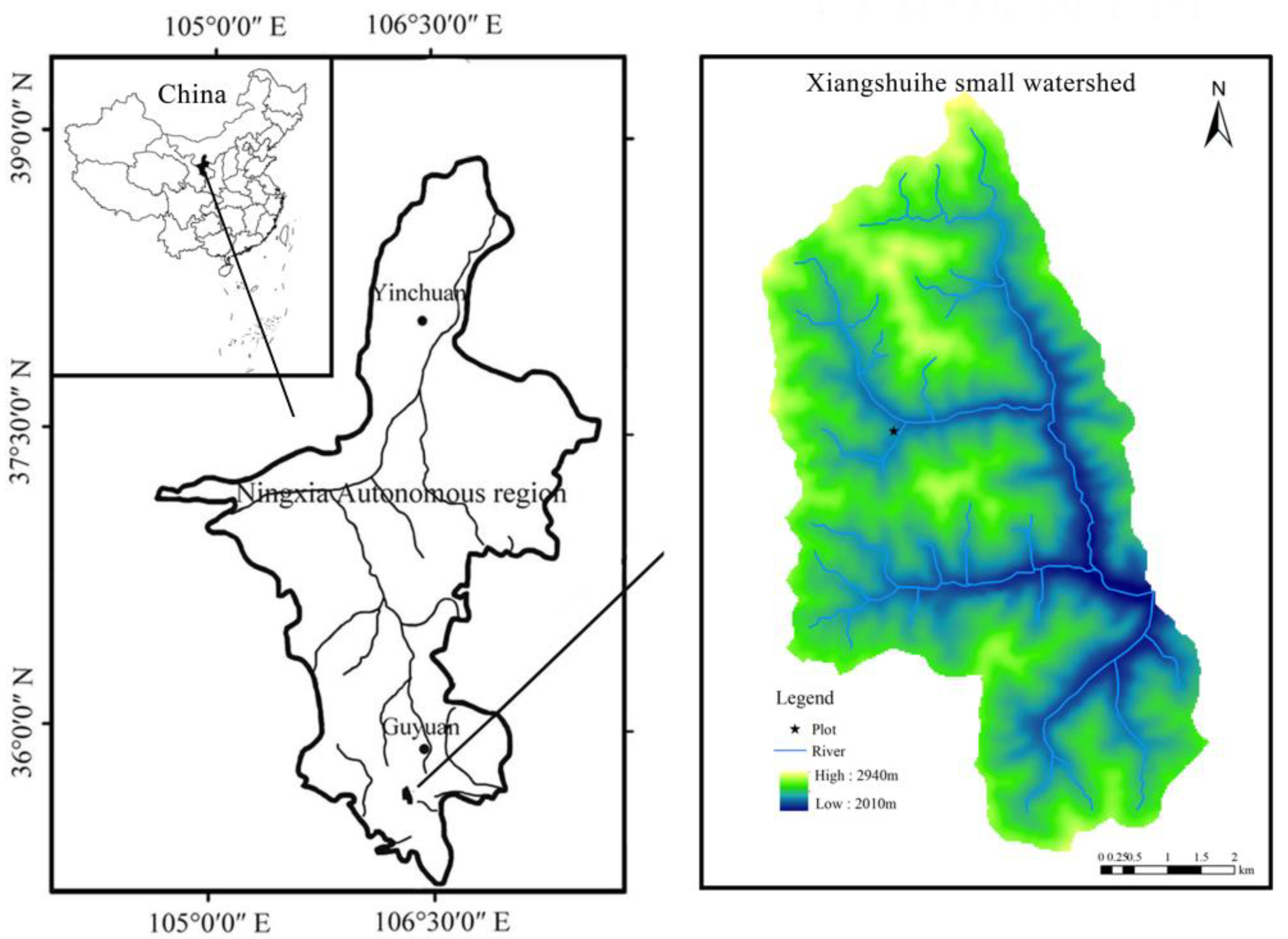
2.1. Study Site and Plant Materials

The study site for this investigation was in the small watershed of Xiangshuihe (106°12′–106°16′ E, 35°27′–35°33′ N) on the east slope of the southern section of the Liupan Mountains in Northwest China, with an area of 43.73 km² and a temperate semi-humid climate (Figure 1). The average annual precipitation is 618 mm, of which 70% occurs from May to October; the average annual temperature is 5.8 ℃; the average annual wind speed is 3.09 m s⁻¹; and the average annual air humidity is 68.8% (1981–2010). The soil type is mainly haplic greyxems soil. Natural secondary forests and artificial forests are the main vegetation types in the small watershed. Secondary forests account for 58% of the area, and the main tree species there are Pinus armandii, Quercus wutaishansea, Betula platyphylla, and B. albosinensis. Planted forests account for 24% of the area, and main tree species there is L. principis-rupprechtii, which accounts for 90% of the total planted forests, with small proportions of P. tabuliformis and Picea asperata.

A 35-year-old plot (106°13′23″ E, 35°30′49″ N) of L. principis-rupprechtii (planted in 1981) was selected for this study. The plot was 30 m (length) × 30 m (width) at an altitude of 2372.6 m with an average slope of 27.7°. Due to the high canopy closure (0.73), the understory shrubs were scattered, covering only approximately 5% of the area, while approximately 40% of this area was covered by the Cotoneaster zabelii herb, as well as, to a lesser extent, Pteridium aguilinum and Carex hancokiana. Specific stand information and soil physical properties for the plot are shown in

Table 1. Stand characteristics and soil physical properties of the 0–60 cm soil layer of the study plot.

Stand Density (stems ha−1)	Canopy Density	DBH (cm)	Tree Height (m)	Clear Length (m)	Canopy Diameter (m)	Soil Bulk Density (cm3 cm−3)	Total Soil Porosity (%)	Field Capacity (%)
815	0.73	19.78	17.87	6.46	3.29	1.05	60.08	35.88

. To measure the canopy diameter, we first set a measuring point on the outer edge of the canopy toward the east, south, west, and north, and then measured the distance between the trunk and the measuring points, ultimately calculating the mean canopy diameter.

2.2. Measurement of Meteorological Factors

A Weatherhawk232 weather station (Weatherhawk, Logan, UT, USA) was set up outside the forest about 100 m away from the sample plot to simultaneously monitor precipitation, air temperature, solar radiation, relative humidity, and wind speed, which were recorded every 5 min.

The comprehensive evaporative pull of the atmospheric environment could be reflected by the reference evapotranspiration (ET_ref, mm d⁻¹), an important index for evaluating forest evapotranspiration/transpiration, which can be calculated using the Penman equation [35], as follows:

$${\mathrm{ET}}_{\mathrm{ref}}=\frac{0.408 \times \Delta { \times (\mathrm{R}}_{\mathrm{n}} - \mathrm{G})+\mathsf{\gamma } \times \frac{900}{{\mathrm{T}}_{\mathrm{a}}+273}{ \times \mathrm{W} \times (\mathrm{E}}_{\mathrm{T}}{ - \mathrm{e}}_{\mathrm{t}})}{\Delta +\mathsf{\gamma } \times (1+0.34 \times \mathrm{W})}$$

(1)

where Δ is the saturated vapor pressure gradient (kPa °C⁻¹); R_n is the solar radiation (w m⁻²); G is the soil heat flux (MJ m⁻² day⁻¹); γ is the psychometric constant (kPa °C⁻¹); T_a is the atmospheric temperature (°C); W is the wind speed (m s⁻¹); E_T is the saturated vapor pressure (kPa); and e_t is the actual vapor pressure (kPa).

2.3. Measurement of Soil Water Content

The root systems for the L. principis-rupprechtii in this study area were mainly distributed in the 0–60 cm soil layer [24], therefore, 5—TE soil moisture, temperature, and electrical conductivity sensors (Decagon, Pullman, WA, USA) were installed in the soil layer at depths of 0–20, 20–40, and 40–60 cm in the sample plot, to monitor the soil volumetric water dynamic changes of the root layer. The data was collected by the EM50 data collector (Decagon, Pullman, WA, USA) every 5 min. The obtained values were further calibrated by soil auge method, and the calibrated VSM varied in the range of 0.19–0.34 cm³ cm⁻³ in the 0–20 cm soil layer, 0.20–0.31 cm³ cm⁻³ in the 20–40 cm soil layer, and 0.16–0.33 cm³ cm⁻³ in the 40–60 cm soil layer during the growing seasons in 2017–2019, respectively. The calibrated VSMs in each soil layer were normalized by calculating the relative soil water content (RSWC) to eliminate systematic errors and increase the comparability of soil water content in each layer. The dimensionless relative soil water content of the i soil layer (RSWC_i, i is 0–20 cm, 20–40 cm, and 40–60 cm, respectively) was calculated as follow:

$${\mathrm{RSWC}}_{\mathrm{i}}=\frac{{\mathrm{VSM}}_{\mathrm{i}}{ - \mathrm{VSM}}_{\min }}{{\mathrm{VSM}}_{\max }-{ \mathrm{VSM}}_{\min }}$$

(2)

where VSM_i is the actual volumetric soil water content of i soil layer (cm³ cm⁻³); VSM_min is the minimum volumetric soil water content in the growing season (cm³ cm⁻³); and VSM_max is the maximum volumetric soil water content in the growing season (cm³ cm⁻³).

2.4. Measurement of LAI

Fifteen fixed measurement points were arranged in a serpentine shape in the sample plot, and the canopy LAI was measured with the LAI-2200c canopy analyser (LI-COR, Lincoln, NE, USA). The measurement frequency was maintained every 9–14 days throughout the growing season, and the LAI of the sample plot was the average of the LAI of 15 fixed measurement points. The daily dynamic variations of LAI are determined by establishing the relationship between measured LAI and the day of the year (DOY) (Figure 2). The fitting function was: LAI = −2.21 × 10⁻⁴ × DOY² + 0.09 × DOY − 5.50 (R² = 0.94, n = 15) in 2017, LAI = −2.13 × 10⁻⁴ × DOY² + 0.09 × DOY − 5.10 (R² = 0.95, n = 13) in 2018, and LAI = −1.92 × 10⁻⁴ × DOY² + 0.08 × DOY − 4.09 (R² = 0.99, n = 11) in 2019.

2.5. Calculation of Sap Flow and T

The stand was divided into four diameter categories based on diameters ≤ 18, ≤18–22, ≤22–26, and ≥26 cm at breast height (DBH). One tree was selected as the sample tree under each diameter category, and the sap flow was observed according to the above diameter classification criteria. The DBH and tree height (H) of the sampling tree were close to the mean DBH and H of the corresponding DBH class. The trunk sap flow density was measured using four-pin SF—L thermal diffusion sap flow probes (Ecomatik, Dachau, Germany) with a probe length of 20 mm, and mounted uniformly on the back of the trunk at 1.30 m from the ground. Prior to installation, hard and aged skin should be removed first from the probe position, and the S₀, S₁, S₂, and S₃ probes should be inserted sequentially into the trunk sapwood within 0–20 mm. The gap between the probe and the trunk was filled with thermally conductive silicone grease to ensure that the probe was fully sensitive to heat. Wrap the trunk at the insertion of the probe with aluminium foil, and the glass glue was applied to the upper aluminium foil and trunk lamination to avoid the effects of solar radiation, mechanical damage and rainwater infiltration on the measurement results. The other end of the probe was connected to a DL2e data logger (Delta-T, Burwell, UK), and data were recorded every 5 min. The sap flow density at the sapwood depth of 0–20 mm (J_s0–20, mL cm⁻² min⁻¹) was calculated as follow [36]:

$${\mathrm{J}}_{\mathrm{s}0–20}=0.714 \times (\frac{{\mathrm{d}}_{\mathrm{tmax}}}{{\mathrm{d}}_{\mathrm{tact}}}-{1)}^{1.23}$$

(3)

$${\mathrm{d}}_{\mathrm{tact}}{=\mathrm{d}}_{\mathrm{t}0} - \frac{{(\mathrm{d}}_{\mathrm{t}1}{+\mathrm{d}}_{\mathrm{t}2})}{2}$$

(4)

where d_tmax is the maximum temperature difference when J_s = 0 (°C); d_tact is the actual temperature difference (°C); d_t0 is the temperature difference between probe S₀ and S₁ (°C); d_t1 is the temperature difference between probe S₂ and S₁(°C); and d_t2 is the temperature difference between probe S₃ and S₁ (°C).

The sapwood thickness of the trees in the plot varied within a small range, and most trees did not exceed 40 mm. When the sapwood thickness was ≤20 mm (corresponding to DBH of 22.5 cm), e.g., the 1st and the 2nd sample trees in the plot (

Table 2. Characteristics of sample trees used to monitor sap flow in the sample plot.

Sample Tree	DBH (cm)	Tree Height (m)	Sapwood Area (cm2)	Canopy Diameter (m)
1	16.0	16.4	200	3.61
2	19.2	17.1	288	4.21
3	24.5	21.6	472	5.07
4	27.1	20.0	576	5.35

), the sap flow density was determined according to the Equation (3); when the sapwood thickness was >20 mm, e.g., the 3rd and the 4th sample trees in the plot, the sap flow density was determined according to using both the sap flow density at the sapwood depth of 0–20 mm (J_s0–20) and 20–40 mm (J_s20–40, mL cm⁻² min⁻¹) [11]. Based on the fitting relationship between J_s0–20 and J_s20–40, the sap flow density at 20–40 mm could be estimated by the following equation:

$${\mathrm{J}}_{\mathrm{s}20–40}={0.7511 \times \mathrm{J}}_{\mathrm{s}0–20 }+0.00071$$

(5)

The mean sap density of sample trees with sapwood thickness >20 mm at 0–40 mm sapwood depth (J_s0–40, mL cm⁻²⋅min⁻¹) was calculated by the following equation:

$${\mathrm{J}}_{\mathrm{s}0–40}=\frac{{\mathrm{A}}_{\mathrm{s}0–20}{ \times \mathrm{J}}_{\mathrm{s}0–20 }{+\mathrm{A}}_{\mathrm{s}20–40}{ \times \mathrm{J}}_{\mathrm{s}20–40}}{{\mathrm{A}}_{\mathrm{s}0–20}{+\mathrm{A}}_{\mathrm{s}20–40} }$$

(6)

where A_s0–20 is the sapwood area of the 0–20 mm (cm²); and A_s20–40 is the sapwood area of the 20–40 mm (cm²).

In this study, four sample trees were selected to estimate the mean sap flow density of the plot. This study used the 2019 data from another Larix principis-rupprechtii plantation plot near the study plot to demonstrate whether four trees can reflect the mean level of sap flow in the plot. Previous studies have confirmed that selecting the number of sample trees with the coefficient of variation (CV) less than 10% for scaling up in the sample plot was acceptable [37,38]. The results showed a CV of 9.13% at a sampling size of four (Supplementary Figure S1), and the stand density in the study plot was higher than that of the sample site. Thinned stands tend to have larger CV values [37], therefore, four sample trees were the minimum sample size that satisfied the scaling up criteria in this study. The mean sap flow density of the sample plot (J_sa, mL cm⁻² min⁻¹) with a small sample size was estimated by weighting the DBH class of the sample tree, as shown in Equation (7):

$${\mathrm{J}}_{\mathrm{sa}}=\frac{{\sum }_{\mathrm{i}=1}^{\mathrm{n}}{\mathrm{J}}_{\mathrm{si}}{\times \mathrm{n}}_{\mathrm{i}} }{\mathrm{N}}$$

(7)

where J_si is the sap flow density of sample tree in the i-th DBH class (mL cm⁻² min⁻¹); n_i is the quantity of sample tree in the i-th DBH class; and N is the total quantity of trees in the plot. The daily canopy transpiration (T, mm) was calculated based on the mean of sap flow rate of the sample trees and total sapwood area of trees in plot, the specific calculation formula was as follow:

$${\mathrm{T}=\mathrm{J}}_{\mathrm{sa}} \times \frac{{\sum }_{\mathrm{i}=1}^{\mathrm{n}}{\mathrm{A}}_{\mathrm{i}}}{\mathrm{S}} \times 60 \times 24 ÷ 1000$$

(8)

where A_i is the sapwood area of the i-th tree in the sample plot (cm²); n is the total number of L. principis-rupprechtii in the sample plot; and S is the sample plot area (m²). The sapwood area of each tree in the sample plot was calculated based on the relationship between the sapwood area and diameter at breast height obtained by the 14 sample trees around the sample plot, as follow: A = 0.2551 × DBH^2.1892 (R² = 0.88).

2.6. Model Establishment

2.6.1. Modified Jarvis-Stewart Model

A Jarvis-Stewart modelling approach [39,40], previously used to simulate canopy conductance, and was further modified to simulate T by Whitley et al. [27] and Li et al. [26]. Three important factors driving T models are ET_ref (reflect atmospheric conditions;), RSWC (reflect soil moisture status), and LAI (reflect canopy structure). One modification has been made in this study, we include the different impact of RSWC of each soil layers, as follows:

$$\mathrm{T}=\mathrm{f} \left({\mathrm{ET}}_{\mathrm{ref}}\right) ·{ [ \mathrm{f} (\mathrm{RSWC}}_{0–20\mathrm{cm}}{)+\mathrm{f} (\mathrm{RSWC}}_{20–40\mathrm{cm}}{)+\mathrm{f} (\mathrm{RSWC}}_{40–60\mathrm{cm}}) ] · \mathrm{f} \left(\mathrm{LAI}\right)$$

(9)

where f(ET_ref) is the response function between T and ET_ref; f(RSWC_0–20cm), f(RSWC_20–40cm), and f(RSWC_40–60cm) are the response functions between T and RSWC in the 0–20, 20–40, and 40–60 cm soil layers; and f(LAI) is the response function between T and LAI.

2.6.2. Determination of the Response Relationship of T to Single Factor and Their Thresholds

The upper boundary line method can describe the single-factor response relationship between variables and is widely used in the establishment of compound models with independent factors as indicators [18,26]. Consequently, the upper boundary line method was used to determine the response functions between T and the ET_ref and LAI in this study. First, ET_ref, REW, and LAI were divided into several segments, and the interval of each segment for ET_ref and LAI was 1 mm d⁻¹ (ET_ref < 1 mm d⁻¹, 1 mm d⁻¹ ≤ ET_ref < 2 mm d⁻¹, 2 mm d⁻¹ ≤ ET_ref < 3 mm d⁻¹, 3 mm d⁻¹ ≤ ET_ref < 4 mm d⁻¹, 4 mm d⁻¹≤ET_ref), 0.2 (RSWC < 0.2, 0.2 ≤ RSWC < 0.4, 0.4 ≤ RSWC < 0.6, 0.6 ≤ RSWC < 0.8, 0.8 ≤ RSWC < 1), and 0.5 (2.5 ≤ LAI < 3, 3 ≤ LAI < 3.5, 3.5 ≤ LAI < 4), respectively. The abscissa of the upper boundary line point was the median of each segment, and the ordinate was calculated using the mean value of T plus the mean value of one standard deviation. The mean value was taken for multiple eligible points in a zone, and each zone had only one upper boundary line point. The change in the median value of the horizontal coordinates of the upper boundary line points in the zone identified the upper boundary line.

When the surface soil moisture area was exhausted, there was still soil moisture in the deep soil layer for absorption, and thus T would not be 0. When the deep soil moisture was 0, there was no more transpiration due to drought (the performance of the upper boundary lines was that the single-factor response intercept of the 0–40 cm soil layer that was not 0, and the 40–60 cm layer was 0).

The threshold of quadratic polynomial relation (i.e., ET_ref threshold for T) is the value of the independent variable (i.e., ET_ref) corresponding to the maximum value of the dependent variable (i.e., T) in the parabola. The threshold of saturated exponential function (i.e., RSWC, and LAI threshold for T) refers to the threshold calculation formula by Wang et al. [41], which was modified based on the threshold formula by Lagergen et al. [42], as shown in Equation (10):

$$\mathrm{R}=\left(\frac{\mathrm{FAC}}{\mathrm{x}}\left(\frac{\left|\mathrm{x} - \mathrm{FAC}\right|}{\left(\mathrm{x} - \mathrm{FAC}\right)}+1\right)+\frac{\left|\mathrm{FAC} - \mathrm{x}\right|}{\left(\mathrm{FAC} - \mathrm{x}\right)}+1\right) \times 0.5$$

(10)

where R is the ratio of observed T to maximum T; FAC is RSWC or LAI; x is the threshold for T.

2.6.3. Calibration and Validation of the Modified Jarvis—Stewart Model

Judging whether the model has application value required a large amount of data verification. In this study, the model was established using the data from 2017 and 2018 and verified using the data from 2019. In addition, the performance of the model was evaluated using the Nash—Sutcliffe efficiency coefficient (NSE), calculated as follows:

$$\mathrm{NSE}=1 - \frac{{\sum }_{\mathrm{i}=1}^{\mathrm{n}}{{(\mathrm{T}}_{\mathrm{o}}^{\mathrm{t}}{ - \mathrm{T}}_{\mathrm{m}}^{\mathrm{t}})}^2}{{\sum }_{\mathrm{i}=1}^{\mathrm{n}}{{(\mathrm{T}}_{\mathrm{o}}^{\mathrm{t}} - \overline{{\mathrm{T}}_{\mathrm{o}}})}^2}$$

(11)

where ${\mathrm{T}}_{\mathrm{o}}^{\mathrm{t}}$ is the actual measured value of canopy T on the t day; ${\mathrm{T}}_{\mathrm{m}}^{\mathrm{t}}$ is the simulated value of canopy T on the t day; and $\overline{{\mathrm{T}}_{\mathrm{o}}}$ is the mean value of the observed value. NSE > 0.6 indicates that the model has good performance in estimating T [38].

2.7. Calculation of the Factor Contribution Rate

The factorial experiment method [10] was used to quantify the relative contribution rates of the RSWCs in the different soil layers to T. The relative contribution rates of the RSWC to T (R_T, %) was calculated with Equation (12):

$${\mathrm{R}}_{\mathrm{T}}=\frac{\Delta {\mathrm{T}}_{\mathrm{i}}}{{\mathrm{f}(\mathrm{control}}_{\mathrm{i}})}\times 100\%$$

(12)

$${\mathrm{f}(\mathrm{control}}_{\mathrm{i}})=\mathrm{f} ({\mathrm{ET}}_{\mathrm{ref}}) ·{ \mathrm{f} (\mathrm{RSWC}}_{\text{i-min}}) · \mathrm{f} \left(\mathrm{LAI}\right)$$

(13)

where ΔT_i is the contribution volume of the RSWC in the i soil layer (i was 0–20, 20–40, and 40–60 cm, respectively) to T; and f(control_i) is the reference T values calculated by the model using the minimum value of RSWC in the i soil layer (RSWC_i-min, 0.04, 0.14, and 0.10 in 0–20, 20–40, and 40–60 cm soil layer, respectively) and the observed ET_ref and LAI.

ΔT_i was calculated by the following equation:

$$\Delta {\mathrm{T}}_{\mathrm{i}}{=\mathrm{T}}_{\mathrm{simulate}}{ - \mathrm{f}(\mathrm{control}}_{\mathrm{i}})$$

(14)

where T_simulate is the simulated T value calculated by the model using the observed ET_ref, RSWC, and LAI.

3. Results

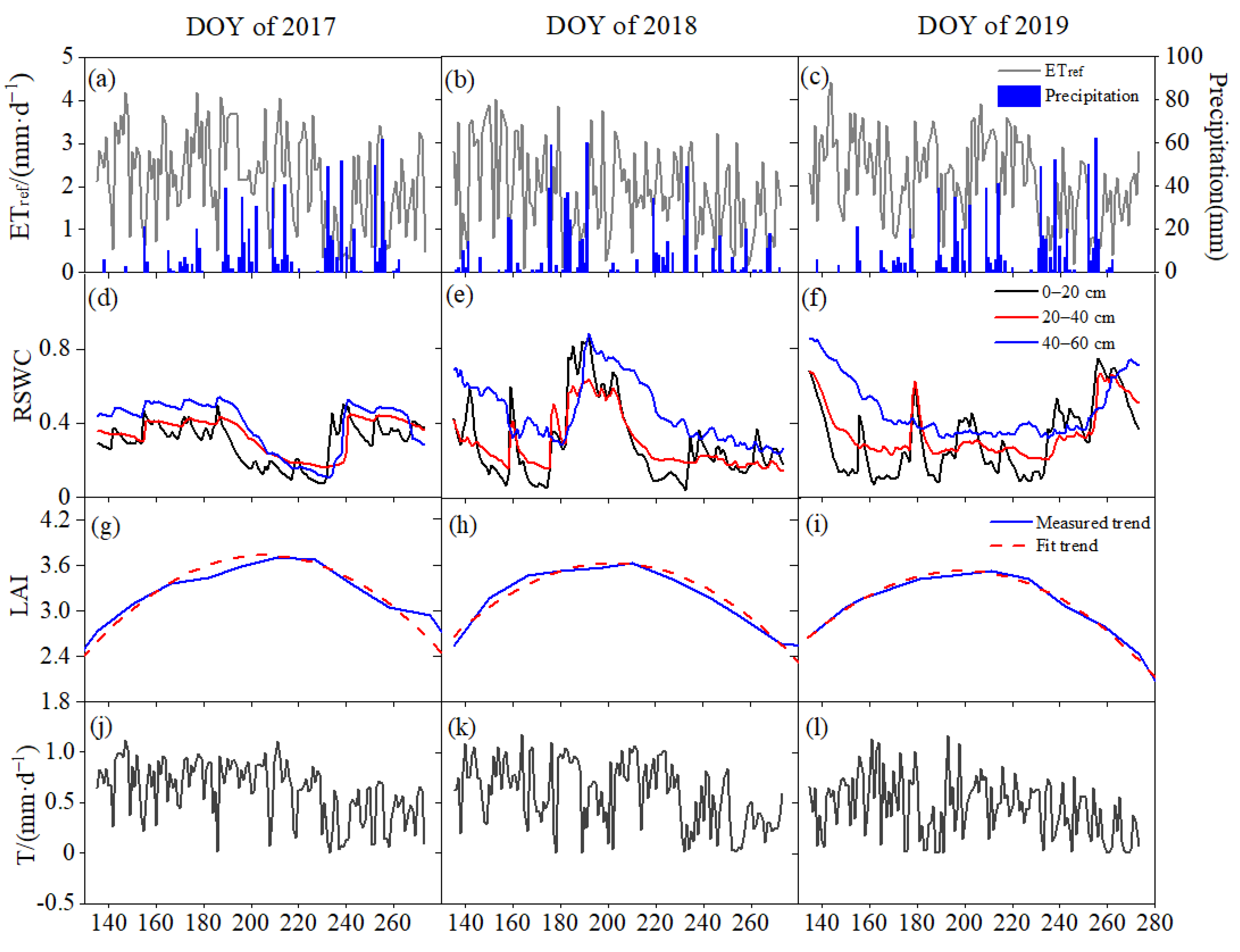
3.1. Variarions of Environmental Conditions and T

Daily variations of the meteorological factors during the three-year study periods (15th May to 30th September) from 2017 to 2019 are shown in Figure 2. There was a clear increasing trend for precipitation during the study period, with 433 mm in 2017, 656 mm in 2018, and 730 mm in 2019 (Figure 2). The total ET_ref was 302.45 mm in 2017, 252.95 mm in 2018, and 293.50 mm in 2019, respectively, with a daily mean of 2.18 mm d⁻¹ in 2017, 1.82 mm d⁻¹ in 2018, and 2.11 mm d⁻¹ in 2019.

RSWC increased with the increase of soil depth in the range of 0–60 cm soil layer, and was 0.30, 0.29, and 0.31 at the 0–20 cm soil depth, 0.34, 0.29, and 0.35 at 20–40 cm soil depth, and 0.39, 0.46, and 0.47 at 40–60 cm soil depth for 2017, 2018, and 2019, respectively.

In 2017–2019, LAI tended to reach its peak in the middle of the growing season (Figure 2). The LAI peaked on the 24 July 2017, the 21 June 2018, and the 18 July 2019, respectively, with a maximum LAI of 3.74, 3.62, and 3.53 in 2017, 2018, and 2019, respectively.

The daily T during the three-year study period fluctuated violently due to the impact of environmental conditions. The range was between 0 and 1.12 mm d⁻¹, 0 and 1.18 mm d⁻¹, and 0 and 1.17 mm d⁻¹, with an average value of 0.62, 0.47, and 0.59 mm d⁻¹, for 2017, 2018, and 2019, respectively.

3.2. T Response to ET_ref, LAI, and RSWC in Different Soil Layers

The upper boundary line shows a significant correlation between T and ET_ref over the three years (Figure 3), and a quadratic function (

Table 3. The response relationship of T to ET_ref, LAI, and RSWC in different soil layers and their thresholds.

Single Factor	Response Relationship	R2	P	n	Threshold
ETref	f(ETref) = a1 × ETref2 + b1 ×ETref	0.99	<0.01	6	3.80
LAI	f(LAI) = a2 − b2 × ec2 × LAI	0.99	<0.01	4	6.24
RSWC0–20cm	f(RSWC0–20cm) = a3 − b3 × ec3 × RSWC0–20cm	0.99	<0.01	6	0.34
RSWC20–40cm	f(RSWC20–40cm) = a4 − b4 × ec4 × RSWC20–40cm	0.98	<0.01	4	0.42
RSWC40–60cm	f(RSWC40–60cm) = a5 − b5 × ec5× RSWC40–60cm	0.99	<0.01	5	0.44

) was found to be a good fit for this data; the relationship between T and LAI showed a similar linear exponential growth trend over the three years (Figure 3), and an obvious functional relationship (Table 3) was identified.

At the 0–60 cm soil depth range, the response of T to the different soil layers RSWC following a saturated exponential function (Figure 4). The T first increased slowly with the increase of RSWC until it reached the threshold, which was 0.34 in the 0–20 cm soil layer, 0.42 in the 20–40 cm soil layer, and 0.44 in the 40–60 cm soil layer. Then the increase showed a tendency to stop gradually. At this time, T reached its maximum response, which was 1.13 mm d⁻¹, 1.13 mm d⁻¹, and 1.17 mm d⁻¹ at the 0–20, 20–40, and 40–60 cm soil layers, respectively. The response functions (Table 3) were determined by the upper boundary line.

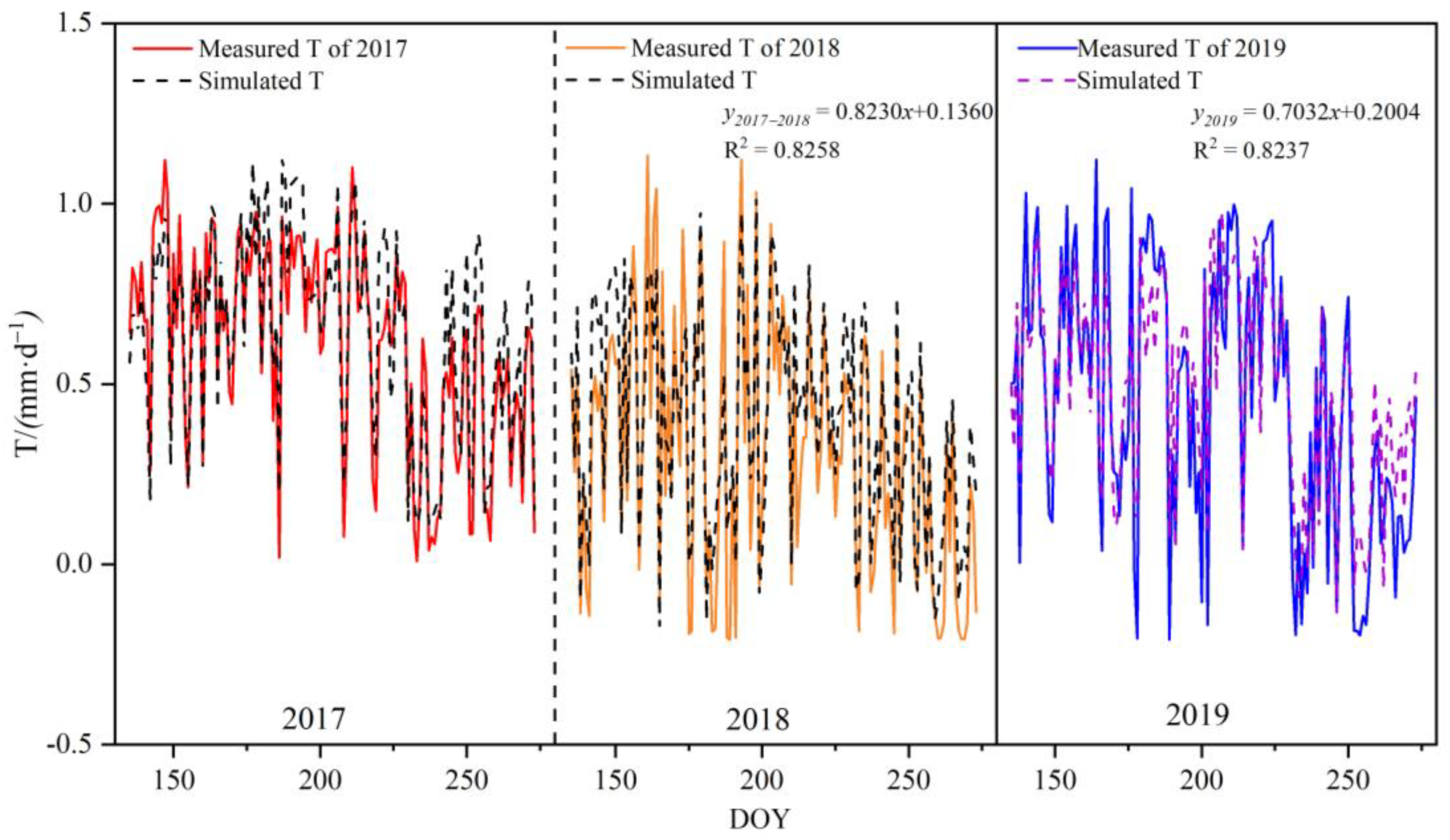
3.3. Model Establishment and Verification

The functions in Table 3 were coupled to obtain a new modified Jarvis—Stewart model in the form of multiplication and accumulation. The model parameters (

Table 4. Parameter values from the optimization of the modified Jarvis—Stewart model.

Parameters	Value	R2	NSE	n
a1	−0.106	0.83	0.82	278
b1	1.284
k (combining a2, a3, and a4)	9.203
b2	1.351
c3	−18.112
b3	16.294
c3	−17.481
b4	0.538
c4	−1.356
b5	0.086
c5	−0.139

) were newly fitted with the 2017–2018 data to form the parameterized T model.

The 2019 data was further used to verify the model’s reliability (Figure 5). The fitting results showed that the T model still kept high simulation accuracy (R² = 0.82, NSE = 0.80, n = 139), and the sum of the simulated T was 248.4 mm during the study period from 2017–2019, slightly higher than the measured T of 232.3 mm.

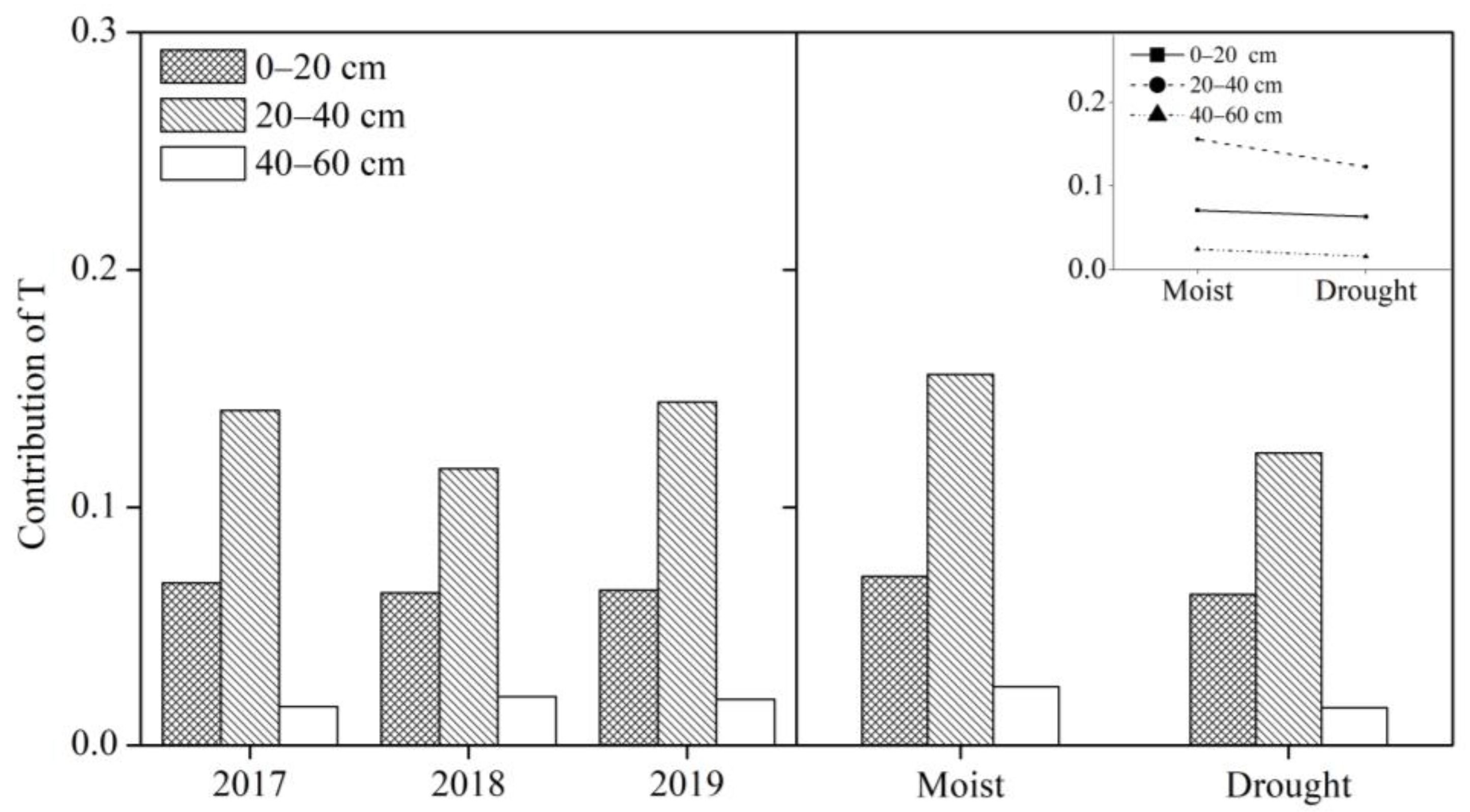
3.4. Contributions of Soil Moisture to T

The contributions of RSWC in the different soil layers to T across different years and moisture conditions are reflected in Figure 6. The law of contribution rate of each soil layer to T was the same in three years, while the rate was RSWC_20–40cm > RSWC_0–20cm > RSWC_40–60cm. Among them, the relative contribution rates varied from 6.4% to 6.8%, 11.6% to 14.4%, and 1.6% to 2.0%, with an average contribution rate of 6.6%, 13.4%, and 1.9% for RSWC_0–20cm, RSWC_20–40cm, and RSWC_40–60cm, respectively.

The relative contribution rates of RSWC of each soil layer to T under differing soil moisture conditions (Moist: RSWC_0–60cm ≥ 0.4; Drought: RSWC_0–60cm < 0.4, RSWC = 0.4 is the threshold value for limiting the T of larch, Supplementary Figure S2) were further analysed (Figure 6). There was no obvious difference among the contribution rates of each soil layer (RSWC_20–40cm > RSWC_0–20cm > RSWC_40–60cm). RSWC_0–20cm, RSWC_20–40cm, and RSWC_40–60cm contributed 7.1%, 15.6%, and 2.5% to T under moist soil condition, and 6.3%, 12.3%, and 1.6% to T under drought soil condition, respectively. There were differences in the decreases in the relative contribution rates of each soil layer as they changed from moist to drought conditions. The contribution rate of RSWC_0–20cm, RSWC_20–40cm, and RSWC_40–60cm decreased by 0.8%, 3.3%, and 0.9%, respectively, showing that as the soil water condition changed from moist to drought, the role of RSWC in the surface soil layer increased compared with other soil layers.

4. Discussion

4.1. A Corresponding Relationship between T and the Major Influencing Factors

Atmospheric condition is the main driving factor of forest T. ET_ref is more representative of the atmospheric influence because ET_ref is a comprehensive index reflecting atmospheric condition [10,26]. ET_ref mainly controls the T by affecting the leaf stomata and the water potential difference between leaves and the atmosphere [18]. With the increase of ET_ref, leaf stomatal gradually open, the stomatal resistance decreased, and T increased. In addition, the rising temperature of the atmosphere and the leaves will increase the water potential difference between the inside and outside of leaves, accelerating T [43]. In turn, when ET_ref is excessive, to prevent water loss, the stomata are closed, increasing the stomatal resistance, ultimately decreasing T [44]. Previous study has found the daily storage water use decreased after ET_ref exceeded a threshold [45]. In this study, there was a significant quadratic relationship to describe the increasing T with rising ET_ref, and the ET_ref threshold was 3.8 mm d⁻¹. However, the ET_ref threshold was not found on several tree species [46,47,48,49,50,51,52]. Whether the ET_ref threshold exists or not, is likely dependent on the physiological regulation of plants [7,53]. In areas with soil water stress, the leaf stomata are more sensitive to water loss, and an inhibitory effect might appear if T reaches a certain threshold to avoid excessive water losses [20,54,55].

In semi-arid or semi-humid areas with seasonal water shortages, soil moisture has a more obvious effect on T [56,57,58]. Soil moisture controls T by adjusting the canopy conductivity and root pressure [10,59]. Severe water stress can even cause xylem embolism to decrease the hydraulic conductivity of the whole tree and limit T [60,61]. However, several studies found no such relationship between soil moisture and T. For example, in Northern China and the Northwest desert transition zone, research on Pinus tabulaeformis, Tamarix chinensis, and Populus euphratica forest found no correlation between soil moisture and T [62,63]. Nevertheless, most studies have found a close relationship between the two. Ji et al. [64] reported that in the desert area of Northwest China, there was a linear relationship between soil moisture and T in Nitraria tangutorum forests. In contrast, another study on L. principis-rupprechtii plantation in a semi-humid area found an exponential relationship between RSWC and T with a threshold of 0.4 [38]. The threshold is generated because soil moisture affects the T generally only within a specific range. When the soil moisture is higher than this threshold, the main limiting factor to T can be the plant physiological activities (e.g., plant hydraulic conductivity. In dry areas where the soil moisture is usually below this threshold, a linear relationship can exist between soil moisture and T. She et al. [65] found that the RSWC threshold under drought conditions was higher than that under moist conditions. In this study, we identified a saturated exponential increase relationship between RSWC_0–60cm and T (Supplementary Figure S2). When the soil moisture was at a high level or relatively high level (e.g., RSWC ≥ 0.4 in this study), the soil water supply for T was sufficient [7,18], thus the RSWC was not a limiting factor to the canopy T. Nevertheless, owing to the limited water transport capacity of trees, the canopy T would not increase with the increase of RSWC. With the decrease of soil moisture (RSWC < 0.4 in this study), the resistance of root water absorption increases [66], and the T gradually decreases. As the soil moisture further decreased, the stomatal leaf close, and root hydraulic conductivity continues to decline [67]. Thus, the canopy T was at a lower level [68]. At this time, soil moisture is the main limiting factor for T. In this study, the response threshold of T to RSWC was 0.4. This threshold was slightly lower than that from the study of Li et al. [26] on the same tree species in semi-arid areas (the threshold of T-RSWC was 0.45), which was consistent with the conclusions of She et al. [65]. However, recent research has also found that the RSWC threshold of Populus tomentosa plantation in northern China was higher under moist than drought conditions [15]. A similar phenomenon was also found in the response threshold of T to different soil layers in this study: The corresponding threshold value is higher in the soil layer with higher RSWC, indicating that the threshold depends not only on soil moisture but also on the range of soil moisture. Although RSWC_40–60cm was the highest in this study, the threshold was larger due to its small range of fluctuation during the growing season.

Distinguish from external influences such as meteorological factors and soil moisture, and canopy LAI is an important indicator as it regulates the transport and dissipation of vegetation water internally [69]. The influence of canopy LAI on T is mainly reflected in the increase in leaf area that creates a larger lighted surface area for water conduction to the canopy, causing an increase in transpiration [70]. Forrester et al. [71] found that the T increased with the rising LAI when LAI < 6. Tie et al. [72] found that T will not increase indefinitely with the increase of LAI. As they found that as LAI increased to 3.5, the trend would gradually slow down. In this study, the response of canopy T to LAI conformed to the saturated exponential pattern, but there is no LAI threshold appearance (the LAI threshold for T was 6.24) in the range of observed data. From the perspective of the T response mechanism, the T will gradually stabilize with the rising LAI, because the mutual shading between leaves causes the canopy light surface area to gradually stabilise with the increase of LAI. In addition, the contraction of the canopy stomata is also a key factor affecting the increase of T with LAI [16]. The number of leaf stomata increases with increasing LAI, and the canopy water delivery capacity increase accordingly, leading to an increase in canopy T [18]; however, when LAI reach a high level, although the number of leaf stomata is still increasing, the plant will shrink the leaf stomata to prevent excessive water loss [67], and thus the canopy T no longer increases with the increase of LAI.

4.2. Contribution of Soil Moisture in Different Soil Layers to T

Previous studies have found that plants use different soil layers in differing ways [73]. This water use strategy is related to the physiological characteristics of the species [30] and soil moisture conditions [18]. For example, the main limiting factor of Populus tomentosa in the North China Plain with sufficient soil moisture is surface soil moisture above 30 cm [15]. Nevertheless, research on the Loess Plateau in China found that Robinia pseudoacacia mainly used deep soil moisture to maintain its normal physiological activities under drought conditions [74]. In this study, the main water sources for T were 0–40 cm soil layers. Plants preferentially utilized water from upper soil layers when soil moisture was sufficient, and otherwise derived water from deep soil layers when upper water is unavailable [75]. In the study years, the precipitation and soil moisture were sufficient, the roots of L. principis-rupprechtii mainly absorbed the water from upper soil layers for T. Additionally, the roots of L. principis-rupprechtii were predominantly distributed in the 10–40 cm soil layer [76], which allowed them to absorb water from upper soil layers during the growing season. In this study, the relative contribution rates of RSWC to each soil layer under drought conditions were significantly lower than those under moist conditions. The study of Pseudotsuga menziesii in the Northern California coast range and Robinia pseudoacacia in the Loess Plateau of China also found a similar pattern [10,77]. Many plant species switched to absorb water mainly from surface to deep soil layers when extreme drought occurred, but some plants would increase the use of surface soil water during drought, for example, in drought conditions before substantial inputs of precipitation in the western United States, the primary source of moisture for Quercus emoryi was surface soil moisture [78]; the efficiency of Quercus variabilis in northern China for water use in the surface soil layers increased from 12.1% to 31.6% as the soil changed from moist to drought conditions [79]. Absorbing surface water might exhibit a high tolerance for limited water source environments [73]. In this study, we found that when the soil moisture conditions changed from moist to drought, the decrease in the contribution rate of the surface soil moisture was lower than that of the deep and middle soil layer. This finding indicated that L. principis-rupprechtii had an increased dependence on surface RSWC compared to other soil layers under drought conditions. Although the soil water content was low during drought in the study years, the surface soil water can still be absorbed to satisfy T requirements. In this case, plants give priority to increase the water absorption from surface soil layer to reduce the energy loss caused by absorbing water from deep soil layers [31]. Additionally, the soil moisture in surface soil layer during drought periods can be supplemented by small rainfall events, allowing the roots to obtain surface soil water.

This study provided a method to quantify the relative contribution rates of soil moisture from the different soil layers to T. Differing from the isotope method, this method can obtain long-term continuous contribution rate data during the growing season and provides a new theoretical framework to conveniently quantify the changes in the relative contribution rates of different soil layers to L. principis-rupprechtii when water conditions are changing.

5. Conclusions

This study has found that the variation of T follows a quadratic relationship with ET_ref, and a saturated exponential increase relationship with RSWC and LAI. When the ET_ref, RSWC, and LAI exceeded their thresholds, the physiological characteristics of plants were the main limiting factors for T. By coupling these response relationships of single factors, a modified Jarvis-Stewart model was established with a good predictive ability. Quantifying the contribution of soil moisture in different soil layers based on the modified Jarvis-Stewart model reveals that the contribution of the RSWC to T is mainly from the surface and middle soil layers. The contributions of the RSWC decreased overall for each soil layer as the soil moisture conditions shifted from moist to drought; however, the decline rate of the contributions indicated that the dependence of T on the water from the surface soil layer is higher than that from the middle and deep soil layers. The modified Jarvis-Stewart model in this study can be used to continuously quantify the contributions of soil moisture across the soil profile to T and provide a model reference and theoretical support for canopy T simulation in the areas with large fluctuations in climate or soil moisture.

References

1. Zhang, Y.Q.; Pena-arancibia, J.L.; Mcvicar, T.R.; Chiew, F.H.S.; Vaze, Z.; Liu, C.; Lu, X.; Zheng, H.; Wang, Y.; Liu, Y.Y. Multi–decadal trends in global terrestrial evapotranspiration and its components. Sci. Rep. 2016, 6, 19124. [Google Scholar] [CrossRef] [Green Version]
2. Erauss, K.W.; Barr, J.G.; Engel, V.; Fuentes, J. Approximations of stand water use versus evapotranspiration from three mangrove forests in southwest Florida, USA. Agric. For. Meteorol. 2015, 213, 291–303. [Google Scholar] [CrossRef]
3. Wang, Y.H.; Yu, P.T.; Feger, K.H.; Wei, X.H.; Sun, G. Annual runoff and evapotranspiration of forestlands and non-forestlands in selected basins of the Loess Plateau of China. Ecohydrology 2011, 4, 277–287. [Google Scholar] [CrossRef]
4. Wang, Q.X.; Wang, M.B.; Fan, X.H.; Zhang, F.; Zhu, S.Z.; Zhao, T.L. Change trends of temperature and precipitation in the Loess Plateau Region of China, 1961–2010. Theor. Appl. Climatol. 2012, 92, 138–147. [Google Scholar] [CrossRef]
5. Jian, S.Q.; Zhao, C.Y.; Fang, S.M.; Yu, K. Effects of different vegetation restoration on soil water storage and water balance in the Chinese Loess Plateau. Agric. For. Meteorol. 2015, 206, 85–96. [Google Scholar] [CrossRef]
6. Yan, W.M.; Deng, L.; Zhong, Y.Q.W.; Shangguan, Z.P. The characters of dry soil layer on the Loess Plateau in China and their influencing factors. PLoS ONE 2015, 10, e0134902. [Google Scholar] [CrossRef] [PubMed]
7. Wang, Y.N.; Cao, G.X.; Wang, Y.H.; Webb, A.A.; Yu, P.T.; Wang, X.J. Response of the daily transpiration of a larch plantation to variation in potential evaporation, leaf area index and soil moisture. Sci. Rep. 2019, 9, 4697. [Google Scholar] [CrossRef]
8. Bhusal, N.; Lee, M.; Lee, H.; Adhikari, A.; Han, A.R.; Han, A.; Kim, H.S. Evaluation of morphological, physiological, and biochemical traits for assessing drought resistance in eleven tree species. Sci. Total Environ. 2021, 779, 146466. [Google Scholar] [CrossRef]
9. Brito, C.; Dinis, L.T.; Moutinho-Pereira, J.; Correia, C.M. Drought stress effects and olive tree acclimation under a changing climate. Plants 2019, 8, 232. [Google Scholar] [CrossRef] [Green Version]
10. Jiao, L.; Lu, N.; Fang, W.W.; Li, Z.S.; Wang, J.; Zhao, J. Determining the independent impact of soil water on forest transpiration: A case study of a black locust plantation in the Loess Plateau, China. J. Hydrol. 2019, 572, 671–681. [Google Scholar] [CrossRef]
11. Tian, A.; Wang, Y.H.; Webb, A.A.; Liu, Z.B.; Yu, P.T.; Xiong, W.; Wang, X. Partitioning the causes of spatiotemporal variation in the sunny day sap flux density of a larch plantation on a hillslope in northwest China. J. Hydrol. 2019, 571, 503–515. [Google Scholar] [CrossRef]
12. Fletcher, A.L.; Sinclair, T.R.; Allen, L.H. Transpiration responses to vapor pressure deficit in well watered ‘slow—wilting’ and commercial soybean. Environ. Exp. Bot. 2007, 61, 145–151. [Google Scholar] [CrossRef]
13. Komatsu, H.; Shinohara, Y.; Kumagai, T.; Kume, T.; Tsuruta, K.; Xiang, Y.; Ichihashi, R.; Tateishi, M.; Shimizu, T.; Miyazawa, Y.; et al. A model relating transpiration for Japanese cedar and cypress plantations with stand structure. For. Ecol. Manag. 2014, 334, 301–312. [Google Scholar] [CrossRef] [Green Version]
14. Xu, X.Y.; Tong, L.; Li, F.S.; Kang, S.Z.; Qu, Y.P. Sap flow of irrigated Populus alba var. pyramidalis and its relationship with environmental factors and leaf area index in an arid region of Northwest China. J. For. Res. 2011, 16, 144–152. [Google Scholar] [CrossRef]
15. Xi, B.Y.; Di, N.; Wang, Y.; Duan, J.; Jia, L.M. Modeling stand water use response to soil water availability and groundwater level for a mature Populus tomentosa plantation located on the North China Plain. For. Ecol. Manag. 2017, 391, 63–74. [Google Scholar] [CrossRef]
16. Xiong, W.; Oren, R.; Wang, Y.H.; Yu, P.T.; Liu, H.L.; Cao, G.X.; Xu, L.H.; Wang, Y.N.; Zuo, H.J. Heterogeneity of competition at decameter scale: Patches of high canopy leaf area in a shade-intolerant larch stand transpire less yet are more sensitive to drought. Tree Physiol. 2015, 35, 470–484. [Google Scholar] [CrossRef]
17. Bucci, S.J.; Scholz, F.G.; Goldstein, G.; Hoffmann, W.A.; Meinzer, F.C.; Franco, A.C.; Giambelluca, T.; Miralles-Wilhelm, F. Controls on stand transpiration and soil water utilization along a tree density gradient in a Neotropical savanna. Agric. For. Meteorol. 2007, 148, 839–849. [Google Scholar] [CrossRef]
18. Liu, Z.B.; Wang, Y.H.; Tian, A.; Webb, A.A.; Yu, P.T.; Xiong, W.; Xu, L.H.; Wang, Y.R. Modeling the response of daily evapotranspiration and its components of a larch plantation to the variation of weather, soil moisture and canopy leaf area index. J. Geophys. Res. Atmos. 2018, 123, 7354–7374. [Google Scholar] [CrossRef]
19. Dekker, S.C.; Bouten, W.; Verstraten, J.M. Modelling forest transpiration from different perspectives. Hydrol. Process. 2015, 14, 251–260. [Google Scholar] [CrossRef]
20. Han, C.; Chen, N.; Zhang, C.K.; Liu, Y.J.; Khan, S.; Lu, K.L.; Li, Y.G.; Dong, X.X.; Zhao, C.M. Sap flow and meteorological about the Larix principis-rupprechtii plantation in Gansu Xinlong mountain, northwestern China. For. Ecol. Manag. 2019, 451, 117519. [Google Scholar] [CrossRef]
21. Wang, H.L.; Tetzlaff, D.; Soulsby, C. Hysteretic response of sap flow in Scots pine (Pinus sylvestris) to meteorological forcing in a humid low-energy headwater catchment. Ecohydrology 2019, 12, e2125. [Google Scholar] [CrossRef]
22. Wu, Y.Z.; Huang, M.B.; David, N.W. Black locust transpiration responses to soil water availability as affected by meteorological factors and soil texture. Pedosphere 2015, 25, 57–71. [Google Scholar] [CrossRef]
23. Granier, A.; Bobay, V.; Gash, J.H.C.; Gelpe, J.; Shuttleworth, W.J. Vapour flux density and transpiration rate comparisons in a stand of Maritime pine (Pinus pinaster Ait.) in Les Landes forest. Agric. For. Meteorol. 1990, 51, 309–319. [Google Scholar] [CrossRef]
24. Ewers, B.E.; Oren, R.; Kim, H.S.; Lai, C.T.; Bohrer, G. Effects of hydraulic architecture and spatial variation in light on mean stomatal conductance of tree branches and crowns. Plant Cell Environ. 2007, 30, 483–496. [Google Scholar] [CrossRef]
25. Hong, L.; Guo, J.B.; Liu, Z.B.; Wang, Y.H.; Ma, J.; Wang, X.; Zhang, Z.Y. Time-lag effect between sap flow and environmental factors of Larix principis-rupprechtii Mayr. Forests 2019, 10, 971. [Google Scholar] [CrossRef] [Green Version]
26. Li, Z.H.; Yu, P.T.; Wang, Y.H.; Webb, A.A.; He, C.; Wang, Y.B.; Yang, L.L. A model coupling the effects of soil moisture and potential evaporation on the tree transpiration of a semi-arid larch plantation. Ecohydrology 2017, 10, e1764. [Google Scholar] [CrossRef]
27. Whitley, R.; Zeppel, M.; Armstrong, N.; Macinnis-Ng, C.; Yunusa, I.; Eamus, D. A modified Jarvis-Stewart model for predicting stand-scale transpiration of an Australian native forest. Plant Soil 2008, 305, 35–47. [Google Scholar] [CrossRef] [Green Version]
28. Llorens, P.; Poyatos, R.; Latron, J.; Delgado, J.; Oliveras, I.; Gallart, F. A multi-year study of rainfall and soil water controls on Scots pine transpiration under Mediterranean mountain conditions. Hydrol. Process. 2010, 24, 3053–3064. [Google Scholar] [CrossRef]
29. Ehleringer, J.R.; Phillips, S.L.; Schuster, W.S.F.; Sandquist, D.R. Differential utilization of summer rains by desert plants. Oecologia 1991, 88, 430–434. [Google Scholar] [CrossRef]
30. Flanagan, L.B.; Ehleringer, J.R.; Marshall, J.D. Differential uptake of summer precipitation among co-occurring trees and shrubs in a pinyon-juniper woodland. Plant Cell Environ. 2010, 15, 831–836. [Google Scholar] [CrossRef]
31. Liu, Z.Q.; Jia, G.D.; Yu, X.X.; Lu, W.W.; Zhang, J.M. Water use by broadleaved tree species in response to changes in precipitation in a mountainous area of Beijing. Agric. Ecosyst. Environ. 2018, 251, 132–140. [Google Scholar] [CrossRef]
32. Leigh, A.; Sevanto, S.; Close, J.D.; Nicotra, A.B. The influence of leaf size and shape on leaf thermal dynamics: Does theory hold up under natural conditions? Plant Cell Environ. 2017, 40, 237–248. [Google Scholar] [CrossRef] [PubMed]
33. Park, G.E.; Lee, D.K.; Kim, K.W.; Batkhuu, N.O.; Tsogtbaatar, J.; Zhu, J.J.; Jin, Y.; Park, P.S.; Hyun, J.O.; Kim, K.S. Morphological characteristics and water-use efficiency of Siberian Elm trees (Ulmus pumila L.) within arid regions of Northeast Asia. Forests 2016, 7, 280. [Google Scholar] [CrossRef] [Green Version]
34. Narayan, B.; Minsu, L.; Ah, R.H.; Areum, H.; Hyun, S.K. Responses to drought stress in Prunus sargentii and Larix kaempferi seedlings using morphological and physiological parameters. For. Ecol. Manag. 2020, 465, 118099. [Google Scholar] [CrossRef]
35. Allen, R.G.; Pereira, L.S.; Raes, D. Crop evapotranspiration: Guidelines for computing crop water requirements. FAO Irrig. Drain. Pap. 1998, 56, 1–15. [Google Scholar]
36. Granier, A. Evaluation of transpiration in a Douglas-fir stand by means of sap flow measurements. Tree Physiol. 1987, 3, 309–320. [Google Scholar] [CrossRef]
37. Čermák, J.; Kučera, J.; Nadezhdina, N. Sap flow measurements with some thermodynamic methods, flow integration within trees and scaling up from sample trees to entire forest stands. Trees 2004, 18, 529–546. [Google Scholar] [CrossRef]
38. Wang, L.; Liu, Z.B.; Guo, J.B.; Wang, Y.H.; Ma, J.; Yu, S.P.; Yu, P.T.; Xu, L.H. Estimate canopy transpiration in larch plantations via the interactions among reference evapotranspiration, leaf area index, and soil moisture. For. Ecol. Manag. 2021, 481, 118749. [Google Scholar] [CrossRef]
39. Jarvis, P.G. The Interpretation of the variations in leaf water potential and stomatal conductance found in canopies in the field. Philos. Trans. R. Soc. Lond. 1976, 273, 593–610. [Google Scholar] [CrossRef]
40. Stewart, J.B. Modelling surface conductance of pine forest. Agric. For. Meteorol. 1988, 43, 19–35. [Google Scholar] [CrossRef]
41. Wang, Y.R.; Wang, Y.H.; Yu, P.T.; Xiong, W.; Du, A.P.; Li, Z.H.; Liu, Z.B.; Ren, L.; Xu, L.H.; Zuo, H.J. Simulated responses of evapotranspiration and runoff to changes in the leaf area index of a Larix principis-rupprechtii plantation. Acta Ecol. Sin. 2016, 36, 6928–6938. [Google Scholar] [CrossRef]
42. Lagergren, F.; Lindroth, A. Transpiration response to soil moisture in pine and spruce trees in Sweden. Agric. For. Meteorol. 2002, 112, 67–85. [Google Scholar] [CrossRef]
43. Novick, K.A.; Ficklin, D.L.; Stoy, P.C.; Williams, C.A.; Bohrer, G.; Oishi, A.C.; Papuga, S.A.; Blanken, P.D.; Noormets, A.; Sulman, B.N.; et al. The increasing importance of atmospheric demand for ecosystem water and carbon fluxes. Nat. Clim. Chang. 2016, 6, 1023. [Google Scholar] [CrossRef] [Green Version]
44. McDowell, N.G.; Pockman, W.T.; Allen, C.D.; Breshears, D.D.; Cobb, N.; Kolb, T.; Plaut, J.; Sperry, J.; West, A.; Williams, D.G.; et al. Mechanisms of plant survival and mortality during drought: Why do some plants survive while others succumb to drought? New Phytol. 2016, 178, 719–739. [Google Scholar] [CrossRef] [PubMed]
45. Sun, L.; Xiong, W.; Guan, W.; Wang, Y.; Xu, L. Use of storage water in Larix principis-ruprechtii and its response to soil water content and potential evapotranspiration: A modeling analysis. Chin. J. Plant Ecol. 2011, 35, 411–421. [Google Scholar] [CrossRef]
46. Caldas, L.; Meinzer, F.C.; Igler, E.; Franco, A.C.; Goldstein, G.; Jackson, P.; Rundel, P.W.; Bustamante, M. Atmospheric and hydraulic limitations on transpiration in Brazilian cerrado woody species. Funct. Ecol. 1999, 13, 273–282. [Google Scholar] [CrossRef]
47. Attia, Z.; Domec, J.C.; Oren, R.; Way, D.A.; Moshelion, M. Growth and physiological responses of isohydric and anisohydric poplars to drought. J. Exp. Bot. 2015, 66, 4373–4381. [Google Scholar] [CrossRef] [PubMed] [Green Version]
48. Gao, Q.; Zhao, P.; Zeng, X.; Cai, X.; Shen, W. A model of stomatal conductance to quantify the relationship between leaf transpiration, microclimate and soil water stress. Plant Cell Environ. 2002, 25, 1373–1381. [Google Scholar] [CrossRef]
49. Vincke, C.; Breda, N.; Granier, A.; Devillez, F. Evapotranspiration of a declining Quercus robur L. stand from 1999 to 2001. I. Trees and forest floor daily transpiration. Ann. For. Sci. 2005, 62, 503–512. [Google Scholar] [CrossRef] [Green Version]
50. Střelcová, K.; Minďáš, J.; Škvarenina, J. Influence of tree transpiration on mass water balance of mixed mountain forests of the West Carpathians. Biologia 2006, 61, 305–310. [Google Scholar] [CrossRef]
51. Wullschleger, S.D.; Hanson, P.J. Sensitivity of canopy transpiration to altered precipitation in an upland oak forest: Evidence from a long-term field manipulation study. Glob. Chang. Biol. 2006, 12, 97–109. [Google Scholar] [CrossRef]
52. Zhang, J.G.; Guan, J.H.; Shi, W.Y.; Yamanaka, N.; Du, S. Interannual variation in stand transpiration estimated by sap flow measurement in a semi-arid black locust plantation, Loess Plateau, China. Ecohydrology 2015, 8, 137–147. [Google Scholar] [CrossRef]
53. Bréda, N.; Cochard, H.; Dreyer, E.; Granier, A. Water transfer in a mature oak stand (Quercus petraea): Seasonal evolution and effects of a severe drought. Can. J. For. Res. 1993, 23, 1136–1143. [Google Scholar] [CrossRef]
54. Ungar, E.D.; Rotenberg, E.; Raz-Yaseef, N.; Cohen, S.; Yakir, D.; Schiller, G. Transpiration and annual water balance of Aleppo pine in a semiarid region: Implications for forest management. For. Ecol. Manag. 2013, 298, 39–51. [Google Scholar] [CrossRef]
55. Bosch, D.D.; Marshall, L.K.; Teskey, R. Forest transpiration from sap flux density measurements in a Southeastern Coastal Plain riparian buffer system. Agric. For. Meteorol. 2014, 187, 72–82. [Google Scholar] [CrossRef]
56. Stephenson, N.L. Climatic control of vegetation distribution: The role of the water balance. Am. Nat. 1990, 135, 649–670. [Google Scholar] [CrossRef]
57. Chang, X.X.; Zhao, W.Z.; He, Z.B. Radial pattern of sap flow and response to microclimate and soil moisture in Qinghai spruce (Picea crassifolia) in the upper Heihe River Basin of arid northwestern China. Agric. For. Meteorol. 2014, 187, 14–21. [Google Scholar] [CrossRef]
58. Wieser, G.; Grams, T.E.E.; Matyssek, R.; Oberhuber, W.; Gruber, A. Soil warming increased whole-tree water use of Pinus cembra at the treeline in the Central Tyrolean Alps. Tree Physiol. 2015, 35, 279–288. [Google Scholar] [CrossRef] [Green Version]
59. Lu, N.; Chen, S.P.; Wilske, B.; Sun, G.; Chen, J.Q. Evapotranspiration and soil water relationships in a range of disturbed and undisturbed ecosystems in the semi-arid Inner Mongolia, China. J. Plant Ecol. 2011, 4, 49–60. [Google Scholar] [CrossRef] [Green Version]
60. Maherali, H.; Pockman, W.T.; Jackson, R.B. Adaptive variation in the vulnerability of woody plants to xylem cavitation. Ecology 2004, 85, 2184–2199. [Google Scholar] [CrossRef]
61. Awad, H.; Barigah, T.; Badel, E.; Cochard, H.; Herbette, S. Poplar vulnerability to xylem cavitation acclimates to drier soil conditions. Physiol. Plant. 2010, 139, 280–288. [Google Scholar] [CrossRef]
62. Zhang, X.M.; Li, X.Y.; Zeng, F.J.; Arndt, S.K.; Bruelheide, H.; Runge, M.; Gries, D.; Foetzki, A.; Thomas, F.M. Water use by perennial plants in the transition zone between river oasis and desert in NW China. Basic Appl. Ecol. 2006, 7, 253–267. [Google Scholar] [CrossRef]
63. Chen, L.X.; Zhang, Z.Q.; Li, Z.D.; Tang, J.W.; Caldwell, P.; Zhang, W.J. Biophysical control of whole tree transpiration under an urban environment in Northern China. J. Hydrol. 2011, 402, 388–400. [Google Scholar] [CrossRef]
64. Ji, X.B.; Zhao, W.Z.; Kang, E.; Jin, B. Transpiration from three dominant shrub species in a desert-oasis ecotone of arid regions of Northwestern China. Hydrol. Process. 2016, 30, 4841–4854. [Google Scholar] [CrossRef]
65. She, D.L.; Xia, Y.Q.; Shao, M.A.; Peng, S.Z.; Yu, S.E. Transpiration and canopy conductance of Caragana korshinskii trees in response to soil moisture in sand land of China. Agrofor. Syst. 2013, 87, 667–678. [Google Scholar] [CrossRef]
66. Takahashi, F.; Kuromori, T.; Urano, K.; Yamaguchi-Shinozaki, K.; Shinozaki, K. Drought stress responses and resistance in plants: From cellular responses to long-distance intercellular communication. Front. Plant Sci. 2020, 11, 556972. [Google Scholar] [CrossRef] [PubMed]
67. Tombesi, S.; Almehdi, A.; DeJong, T.M. Phenotyping vigour control capacity of new peach rootstocks by xylem vessel analysis. Sci. Hortic. 2011, 127, 353–357. [Google Scholar] [CrossRef]
68. Bhusal, N.; Han, S.G.; Yoon, M.T. Impact of drought stress on photosynthetic response, leaf water potential, and stem sap flow in two cultivars of bi-leader apple trees (Malus × domestica Borkh.). Sci. Hortic. 2019, 246, 535–543. [Google Scholar] [CrossRef]
69. Parker, G.G. Tamm review: Leaf Area Index (LAI) is both a determinant and a consequence of important processes in vegetation canopies. For. Ecol. Manag. 2020, 447, 118496. [Google Scholar] [CrossRef]
70. Poyatos, R.; Llorens, P.; Piol, J.; Rubio, C. Response of Scots pine (Pinus sylvestris L.) and pubescent oak (Quercus pubescens Willd.) to soil and atmospheric water deficits under Mediterranean mountain climate. Annu. For. Sci. 2008, 65, 306. [Google Scholar] [CrossRef]
71. Forrester, D.I.; Collopy, J.J.; Beadle, C.L.; Warren, C.R.; Baker, T. Effect of thinning, pruning and nitrogen fertiliser application on transpiration, photosynthesis and water-use efficiency in a young Eucalyptus nitens plantation. For. Ecol. Manag. 2012, 266, 286–300. [Google Scholar] [CrossRef]
72. Tie, Q.; Hu, H.C.; Tian, F.Q.; Guan, H.D.; Lin, H. Environmental and physiological controls on sap flow in a subhumid mountainous catchment in North China. Agric. For. Meteorol. 2017, 240, 46–57. [Google Scholar] [CrossRef]
73. Asbjornsen, H.; Shepherd, G.; Helmers, M.; Mora, G.D. Seasonal patterns in depth of water uptake under contrasting annual and perennial systems in the Corn Belt Region of the Midwestern U.S. Plant Soil 2008, 308, 69–92. [Google Scholar] [CrossRef]
74. Zhao, Y.L.; Wang, Y.Q.; He, M.N.; Tong, Y.P.; Zhou, J.X.; Guo, X.Y.; Liu, J.Z.; Zhang, X.C. Transference of Robinia pseudoacacia water-use patterns from deep to shallow soil layers during the transition period between the dry and rainy seasons in a water-limited region. For. Ecol. Manag. 2020, 457, 117727. [Google Scholar] [CrossRef]
75. Wang, J.; Fu, B.J.; Lu, N.; Zhang, L. Seasonal variation in water uptake patterns of three plant species based on stable isotopes in the semi-arid Loess Plateau. Sci. Total Environ. 2017, 609, 27–37. [Google Scholar] [CrossRef] [PubMed]
76. Zhang, Y.P.; Jiang, Y.; Wang, B.; Jiao, L.; Wang, M.C. Seasonal water use by Larix principis-rupprechtii in an alpine habitat. For. Ecol. Manag. 2018, 409, 47–55. [Google Scholar] [CrossRef]
77. Link, P.; Simonin, K.; Maness, H.; Oshun, J.; Dawson, T.; Fung, I. Species differences in the seasonality of evergreen tree transpiration in a Mediterranean climate: Analysis of multiyear, half-hourly sap flow observations. Water Resour. Res. 2014, 50, 1869–1894. [Google Scholar] [CrossRef]
78. Weltzin, J.F.; Mcpherson, G.R. Spatial and temporal soil moisture resource partitioning by trees and grasses in a temperate Savanna, Arizona, USA. Oecologia 1997, 112, 156–164. [Google Scholar] [CrossRef]
79. Liu, Z.Q.; Yu, X.X.; Jia, G.D. Water utilization characteristics of typical vegetation in the rocky mountain area of Beijing, China. Ecol. Indic. 2018, 91, 249–258. [Google Scholar] [CrossRef]
Figure 1. Xiangshuihe small watershed and study plot location.
Water 13 02720 g001
Figure 2. Daily variations of environmental factors (ETref and precipitation (ac), RSWC at a depth of 0–20, 20–40, 40–60 cm (df), LAI (gi), and T (jl)) during the study periods in the plot of L. principis-rupprechtii from 2017 to 2019.
Water 13 02720 g002
Figure 3. Response of T to ETref and LAI from 2017 to 2019.
Water 13 02720 g003
Figure 4. Response of T to different soil layers RSWC (0–20, 20–40, and 40–60 cm) from 2017 to 2019.
Water 13 02720 g004
Figure 5. Comparison of the measured and simulated T values during the calibration (2017–2018) and validation (2019) phase.
Water 13 02720 g005
Figure 6. Relative contribution rates of RSWC0–20cm, RSWC20–40cm, and RSWC40–60cm to T under different years and moisture conditions (moist or drought).
Water 13 02720 g006