1. Introduction
The offshore platform is a central facility for offshore oil extraction, transportation, observation, navigation, and construction. In summary, an offshore platform is the base for offshore production, operation, and life. The pile leg is a vital structure to support the offshore platform, but damage to the pile leg caused by drag is enormous. So how to effectively reduce the drag and the structural vibration to prolong the service life of offshore platform pile legs has become an important research topic.
The drag is related to vortex shedding in the wake of the cylinder. Moreover, it is most dangerous when the cylinder’s vibration frequency is close to the natural frequency. Therefore, the suppression of drag can be considered from two aspects: avoiding the natural frequency of the structure, or suppressing the formation and development of vortices. Of course, some measures can make both results occur simultaneously. Some methods can reduce the drag of the system and avoid sympathetic vibration while suppressing the vortex.
So far, there has been much research on the reduction of cylinder drag. For example, Muddada and Patnaik [
1] significantly reduced the drag induced by eddy current. The method they used was to control the wake vortices by adding two small control cylinders to the rear of the forced cylinder, and the technique was based on the simple active flow control strategy of momentum injection. Owen and Bearman [
2] conducted an experimental analysis of drag reduction characteristics of risers across a broad Reynolds number range. They found that, when the cylinder was attached with a sinuous axis, the suppression of vortex shedding and drag reduction rate reached up to 47%, and about 25% for the cylinder with bumps. Moreover, Ivo Amilcar [
3] studied the acceleration of drag and the control effect of the bio-cylinders’ flow structure based on a harbor seal vibrissa, then proved that the bionic surface changed the characteristics of drag of the cylinder. It was also found that the bionic surface could reduce the drag of the cylinder at a certain wind attack angle, and the eddy scale and the turbulent kinetic energy (TKE) in the wake area decreased. In the experiment of Wang et al. [
4], the drag reduction test of the wavy cylinder in the
Re range of 2.0 × 10
4 to 5.0 × 10
4 was carried out. They demonstrated that the average drag coefficient of the wavy cylinder with different inclinations was less than that of the smooth cylinder. The maximum drag reduction rate could reach more than 20%, and the surface inclination of a wavy cylinder was an important parameter affecting its drag reduction effect.
Based on the above existing studies, it can be seen that the control of the flow drag of the pile legs of the offshore platform can be, ultimately, simplified to the study of the cylindrical flow phenomenon. However, these studies have significantly changed and complicated the circular structure, increasing the cylinder mass. If these devices are applied in the pile leg, its design and installation process will be confused. Further research has greatly improved the above problems by using these conclusions [
5,
6]. They considered that the non-smooth surface could reduce the drag of a plane or cylindrical surface. Many studies have proved that a grooved surface and dimpled surface have good drag reduction ability. In earlier studies, Oki et al. [
7] found through numerical simulation that the addition of grooves on the cylinder’s surface would lead to the backward movement of the separation point of the cylinder, the reduction of pressure difference and the reduction of drag. Takayama and Aoki [
8] mainly discussed the influence of groove depth on force coefficient and backflow by carrying out this experiment and analyzing the results.
Concerning the dimpled structure, Zhou et al. [
9,
10] had already made a comprehensive study of the drag reduction characteristics of the dimpled structure when
k/D = 0.05 (
k/D is the roughness coefficient). The
and the root mean square of lift coefficient (
Clrms) of the dimpled cylinder decreased within the range of
Re = 7.4 × 10
3~8 × 10
4, and the reduction rate was between 10% and 30%. The distribution position of dimples on the surface of the cylinder also affected the drag. On the other hand, Wang et al. [
11] used the shear stress transport (
SST k-ω) turbulence model to conduct numerical simulation analysis to discuss the influence of the dimpled structure’s parameters on the drag reduction. Finally, it was concluded that the dimple depth’s impact is more significant than other factors, and a circular dimple had a better drag reduction effect than a spherical dimple.
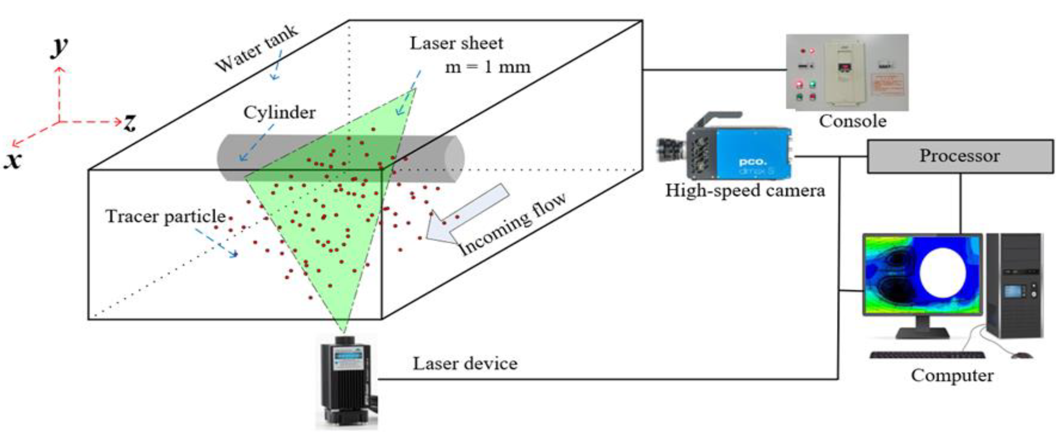
Based on the above research, this paper aims to control vortex formation and development in order to reduce the drag by placing dimples on the cylinder surface. A dimple of circular model and k/D = 0.005 will be decorated on the surface of the cylinder to suppress the vortex. Numerical simulation and PIV technique are used to study drag reduction characteristics. This study focuses on the drag reduction effect and mechanism of the circular cylinder with the dimpled surface in terms of drag reduction rate, force coefficient, Strouhal number, flow velocity, and flow structure.
2. Numerical Simulation Method
2.1. Turbulence Model and Transition Model
For the incompressible viscous fluid, the following formulas can express its governing equations [
12]:
Here, ui is the velocity component of the fluid in the direction xi, in two dimensions, i, j = 1, 2. u1 = u and u2 = v are the horizontal and vertical velocity components, respectively. t and p represent the flow time and pressure. Re (=ρU∞D/μ) is the Reynolds number. ρ, U∞, D, and μ are the fluid density, fluid velocity, cylinder diameter, and the viscosity coefficient.
To describe the turbulent flows, the RANS (Reynolds-averaged Navier-Stokes) equation is usually used instead of the N-S (Navier-Stokes) equation. The RANS equation is obtained by homogenizing the N-S equation, as described in the following:
Here, and are time-averaged velocities, and represent fluctuating velocities, μt is the turbulent viscosity coefficient, k is the turbulent kinetic energy, and δij is the Kronecker delta symbol. (the Reynolds stress term) in the equation makes the RANS system no longer closed, so the turbulence model is needed to make the stress term closed based on Boussinesq’s assumption.
The boundary layer velocity gradient is large for the flow around the cylinder, so the SST (shear stress transport)
k-
ω two-equation turbulence model is a better choice [
12]. The SST
k-
ω turbulence model contains two equations of turbulent kinetic energy (
k) and dissipation rate (
ω):
where
σk and
σω are the turbulent Prandtl numbers about
k and
ω,
μt is the turbulent viscosity coefficient,
is the effective rate of turbulent kinetic energy generation,
Pω is the rate of turbulent dissipation,
β*(
β* = 0.09) is the model constant, and
F1 is the mixing function.
The boundary layer still shows laminar separation for the flow around the cylinder within the subcritical region (300 < Re < 3 × 10⁵), while turbulent vortex streets already exist in the wake. This paper combines a transition model based on the above turbulence model to simulate the transition.
The transition SST four-equation transition model is based on the coupling of transport equations about
γ (intermittent factor) and
(momentum thickness Reynolds number), relevant empirical formulas, and the SST
k-
ω two-equation turbulence model. The transport equations of
γ and
can be expressed as [
13]:
where
σγ,
σθt,
Ca1,
Ca2,
Ce1,
Ce2, and
cθt are the transition constants,
Flength is the transition length function,
Fonset and
Fturb are the transition control functions,
Fθt is the switching function, and
S,
Ω,
T, and
Reθt represent the strain rate, the vorticity, the time scale, and the critical momentum thickness Reynolds number respectively. The empirical correlation function and model parameters of the transition model can be referred to as in the study of Langtry et al. [
14,
15,
16].
The Transition-SST model can capture flow variation sensitively when the Reynolds number is more abundant. For example, it can represent flow separation and pressure gradient change well. The model can also observe the near-wake of the cylinder’s flow characteristics and even predict the transition of the boundary layer well [
12].
2.2. Computational Domains and Boundary Conditions
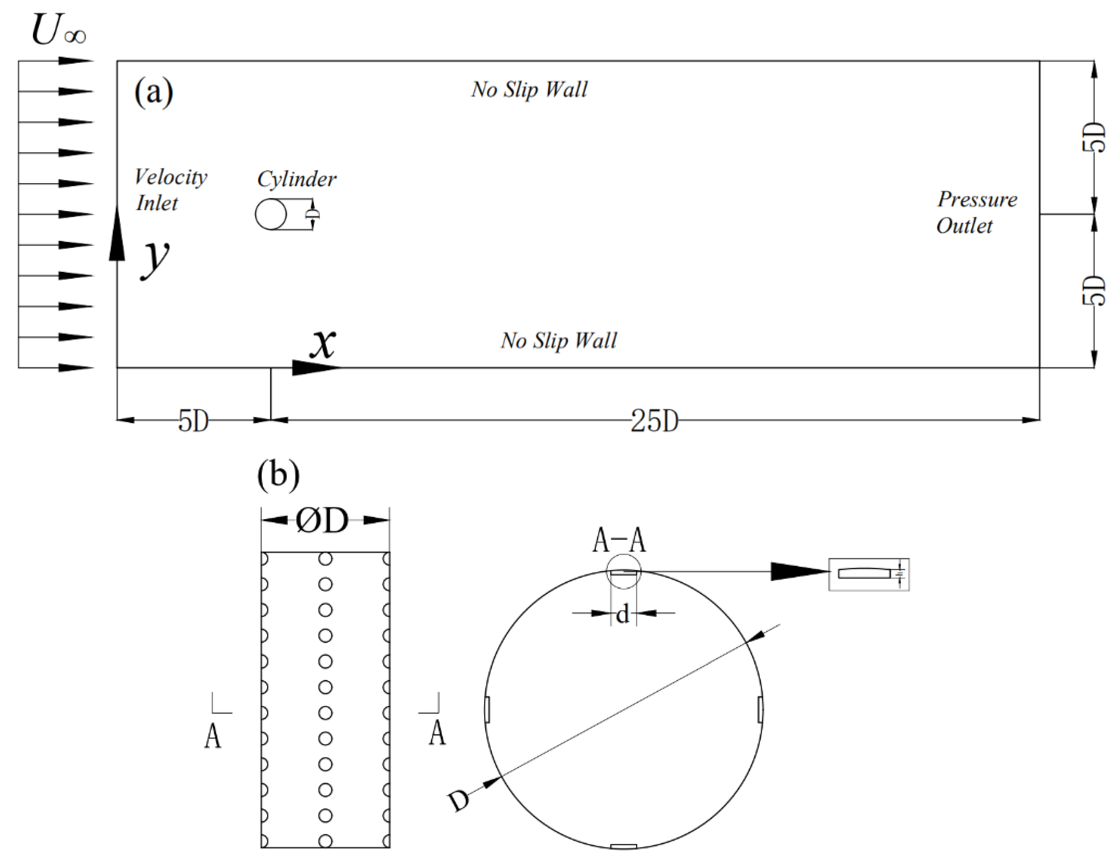
The numerical simulations carried out in this paper shared the same computational domain, as shown in
Figure 1a. The domain size is determined based on the study by Sarker [
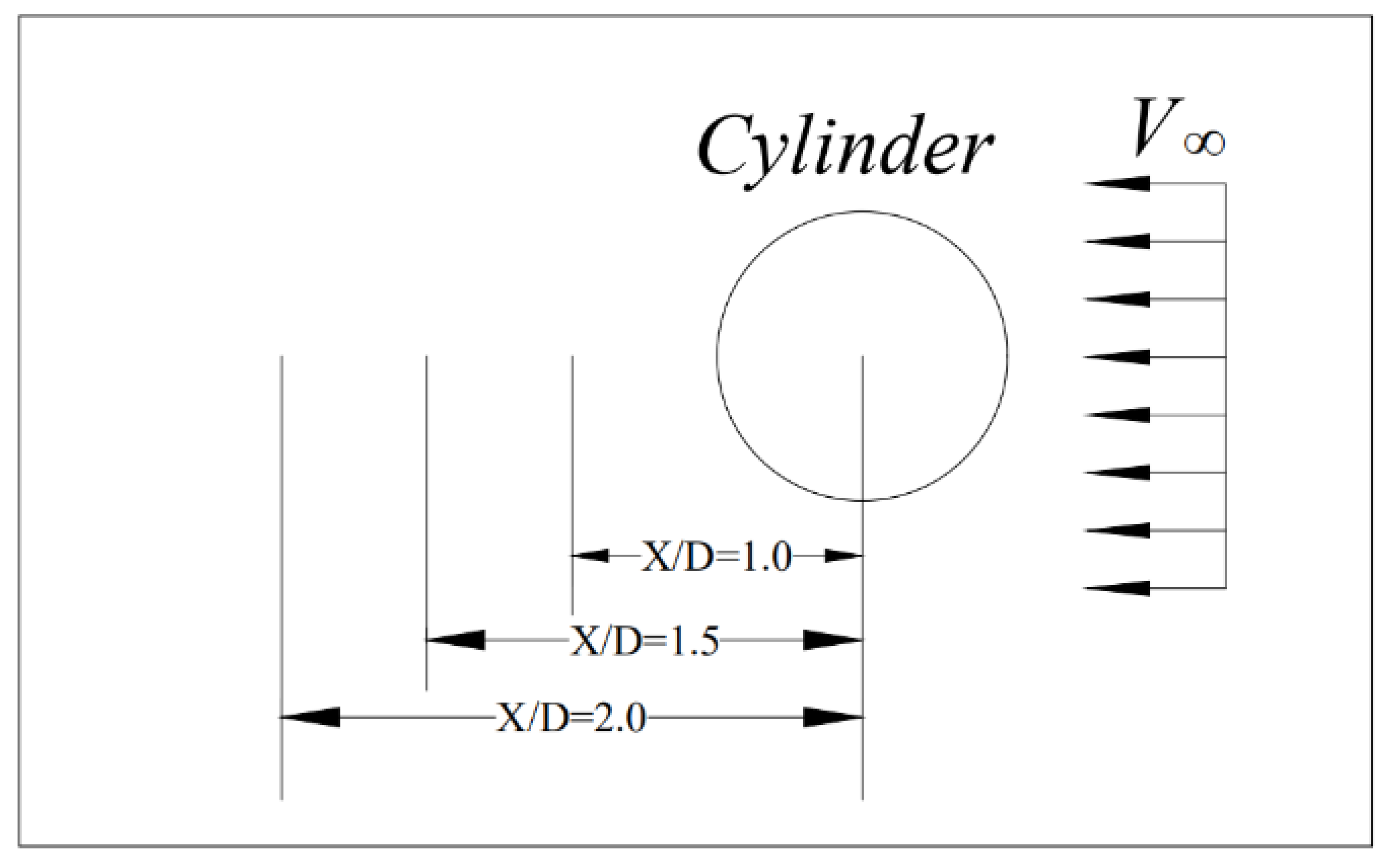
17]. According to Sarker’s research, the distance from the flow field’s outlet to the cylinder’s center should be no less than 12D, which would ensure the disappearance of the cylinder’s influence on the fluid. To better observe the flow field’s backflow, the distance from the basin outlet to the center of the cylinder was set to 25D. The gap between the basin inlet and the cylinder’s center was 5D, and the distance between the cylinder’s center and the two sides of the wall was 5D. Finally, a rectangle computational domain of 30D (in the streamwise direction) × 10D (in the transverse direction) was adopted for 2D numerical simulations.
The boundary conditions of the computational domain are also known from
Figure 1a. For all simulations, the flow field’s inlet and outlet are the velocity inlet boundary and the pressure outlet boundary, respectively. The front and back are no-slip walls, and the cylinder is a fixed wall boundary. The geometric model above uses the two-dimensional rectangular coordinate system for this computational domain. In this coordinate system,
x and
y denote the streamwise and transverse directions of the flow field.
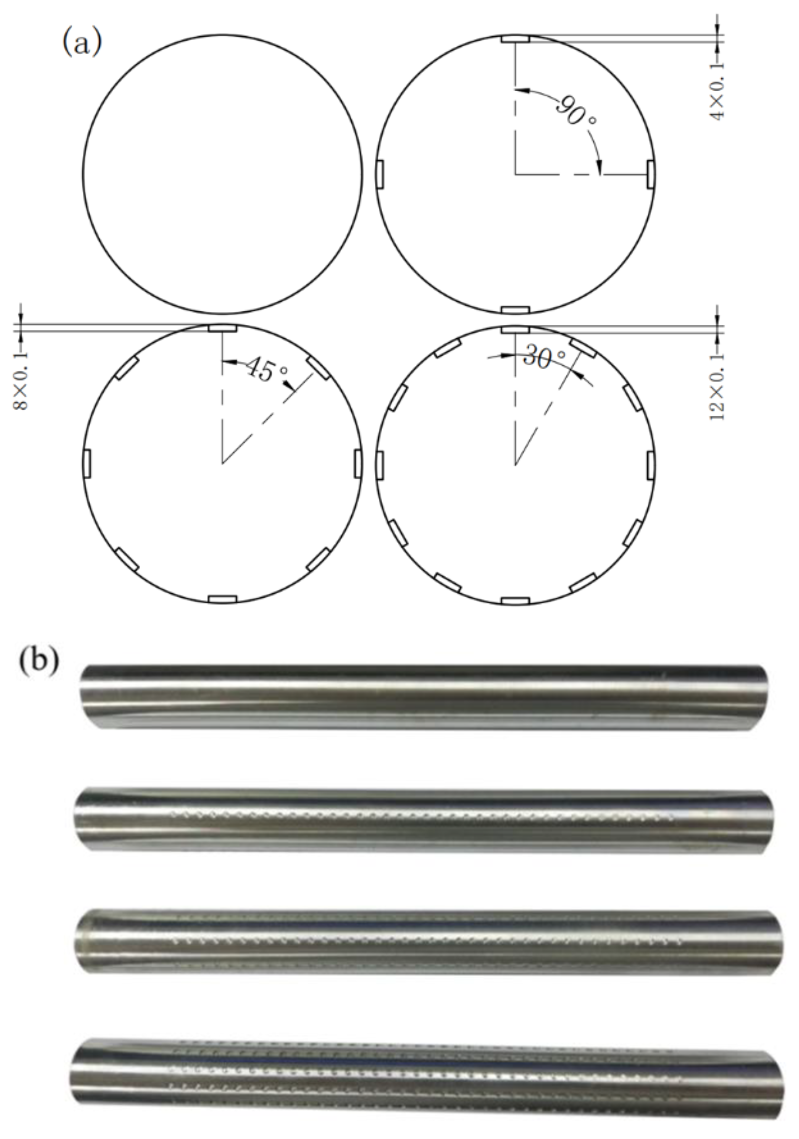
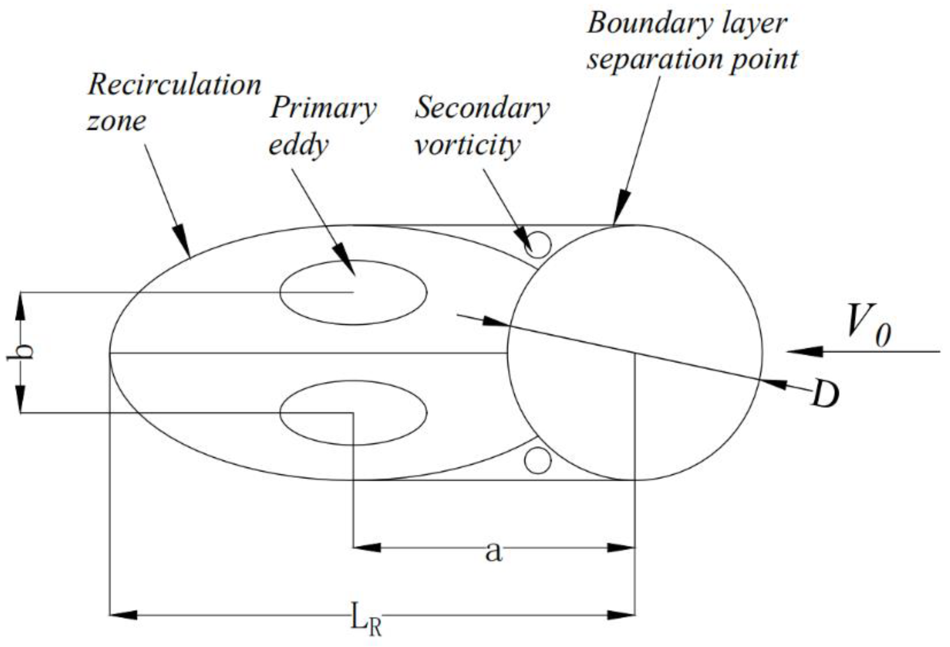
Figure 1b is a schematic diagram of the dimpled structure.
D (
D = 20 mm),
h, and
d are the cylinder’s diameter, dimple’s depth, and the dimple’s diameter (
d = 2 mm,
d/
D = 0.1), respectively.
Table 1 provides the simulation cases and parameters covered. The number of dimple columns controlled the number of dimples. The dimples were evenly distributed on the surface of the cylinder in an equiangular manner. The distribution of dimples in four columns, for example, is given in
Figure 1b. The relevant parameters of
Re are obtained from the investigations [
18,
19,
20,
21]. The pile leg’s diameter was set as 0.5 m, and the environmental flow velocity of the pile leg was 0.2 m/s and 0.4 m/s. To sum up, the values of Reynolds number are
Re1 = 1 × 10
5 and
Re2 = 2 × 10
5, respectively.
h is estimated by the formula of boundary layer thickness [
22,
23] (
h = 0.035
DRe − 1/7). To control the cylinder’s roughness, the value of
k is equal to 0.1 mm. That is,
k/
D = 0.005 (
k/
D is the roughness coefficient, and
k =
h is the dimple’s depth).
2.3. Computational Mesh
In the region near the cylindrical wall, the gradient of the average velocity is considerable. In a very short reasonable distance from the wall, the relatively large velocity value is suddenly reduced to the same velocity value as the wall. Due to such phenomena, the simulation of the flow around a cylinder needs treatment of the near-wall [
22,
24]. Since the Transition-SST turbulence model is adopted in this paper, it is usually required to meet
y+ ≈ 1. The relation between
y+ and the height of the first layer mesh can be expressed as [
25]:
Here, Δy is the height of the first layer mesh, and D is the cylinder’s diameter. Calculated by the formula, the height of the first layer mesh of the two models in this paper is 0.004 mm and 0.0021 mm. During the dividing of the grid, the height of the first layer mesh was set to 0.001 mm.
After finishing the above work, grid independence verification was undertaken. Four different meshes for the smooth cylinder and the dimple cylinder at
Re = 1 × 10
5 were checked. The number of cells was controlled by the grid expansion ratio and the number of nodes.
Table 2 and
Table 3 summarize the verification results, providing the dependence of the
(
is the time-averaged drag coefficient.
Cd =
Fd/0.5
ρU∞2A, where
Cd is the drag coefficient,
Fd is the drag of the cylinder,
ρ is the fluid density,
U∞ is the flow velocity, and
A is the upwind area), and
Clrms is the root mean square of lift coefficient.
), and the Strouhal number
St (
St =
fD/
U∞, where
f is the vortex shedding frequency,
D is the cylinder diameter,
U∞ is the flow velocity) on the mesh size. The three values converged at M3 and M3′. It can be seen that the data differences between M3 and M4 or M3′ and M4′ are around 0.32%, indicating that a further increase of mesh resolution would have a negligible effect on the results of the numerical simulation [
26]. In the end, the mesh size of M3 (for the smooth cylinder) and M3′ (for the dimple cylinder) was adopted in this simulation, the grid expansion ratio was kept below 1.1, and the time step size was controlled below 4 × 10
−4 s. The results of the meshing are shown in
Figure 2. For the smooth cylinder, this mainly controls the area with dense meshes, while for the cylinder with dimples, it is vital to separate the dimples separately for grid division.
2.4. Parameter Verification
The parameter verification was performed for the smooth cylinder at
Re = 1 × 10
5 to verify the accuracy of the turbulence model. The parameters include
and
St, and the experimental data came from the research of Schewe [
27] and Zdravkovich [
28]. According to
Table 4, the values of
and
St in the numerical simulation are very close to the experimental values, indicating that the results of the turbulence model are highly reliable.
2.5. Numerical Simulation Parameters Setting
Based on the above work, the basic setup for fluid computing software can be selected as follows, as tabulated in
Table 5. In the table, it can be obtained that the solver is a pressure-based transient solver, the pressure-velocity coupling scheme is SIMPLEC, and the solution format is the second-order upwind format.


