1. Introduction
Hydrological monitoring is recognized as one of the most important factors in hydrology and flood risk management [
1,
2]. However, runoff model parameters are usually estimated on the basis of recommendations or guidelines from user manuals and literature, although accurate and reliable model results can be achieved using good quality hydrologic data from a well-designed and well-implemented data collection program [
1,
3]. Furthermore, real-time hydrological monitoring will be needed to explain the nature of dynamical hydrologic systems, ecohydrology, and vegetated flows, to help with decision making aiming to mitigate flood risk, among other things [
1,
4,
5,
6].
Moreover, the goals of the current International Hydrologic Scientific Decade 2013–2022 [
7] highlight these challenges, and call for the development of new and innovative monitoring techniques to improve hydrologic monitoring platforms, networks, and databases [
4]. Nevertheless, it is still a challenge for researchers to collect real-time data, given the high costs of conventional data acquisition systems, which hinder the continuous hydrologic monitoring networks in extended areas and developing countries [
4].
According to Paul and Buytaert [
3], there has been a decline in the amount of hydrological data collected worldwide. In general, the gauging stations in small catchment basins are solely installed in a few locations, and they gather data at low frequencies. Thus, extreme events, which have the potential to cause severe damage, are scarcely documented, leading to difficulties in flood modelling and forecasting [
8,
9].
The need for hydrological data around the world is difficult to achieve with traditional monitoring strategies, due to their high costs. Within this framework, a new and promising generation of low-cost sensors for hydrologic monitoring, logging, and transition has been born [
4,
10,
11]. Such sensors open the door for extended smart monitoring networks and improved data coverage, but also enhanced sustainability at a time when monitoring networks are globally in decline [
3].
Low-cost sensors have already been used in research for a variety of applications [
12,
13,
14,
15,
16,
17,
18,
19]. Those of interest are the ones regarding water monitoring, such as water quality monitoring [
1,
4,
8,
20,
21,
22,
23,
24,
25,
26,
27]; soil water content measurement [
28,
29]; water level and flow hydraulic properties [
8,
30,
31]; and hydrological monitoring systems [
2,
4,
5,
23,
26,
32]. However, there are still gaps to be overcome for this technology to be reliable.
According to Trubilowicz et al. [
26], low-cost and low-power wireless sensor networks have the potential to revolutionize data collection methods in hydrology, which, in addition to the open-hardware philosophy in analogy with the concept of open source software, aims at providing free and transparent access to hardware design, projects, and code so that users can easily share, customize, and upgrade their systems [
33]. A smart monitoring multi-sensor network, in order to be reliable, must be able to store, retrieve, and remotely transmit large amounts of widespread data at a very high frequency [
1,
34]; and the use of wireless sensor networks (WSN) will be the main option for field monitoring in a multi-node monitoring network [
24,
35]. WSNs have become a critical part of environmental monitoring; they have been widely studied and deployed in real-life operations [
4], such as in flood disaster preventions, an area in which there has been unprecedented government support for research [
1].
There is a wide variety of sensors that can be used for hydrological monitoring. For example, to monitor water level, we have contact and non-contact water level sensors; the former need to be in contact with water and can be damaged by the debris flow and torrential water behavior that characterize small mountain basins, such as that proposed by Kevin Sze Chiang Kuang [
30], based on plastic optical fiber or immersed pressure sensors. Consequently, non-contact water level sensors based on radar or ultrasound seem to be a better option for these locations, especially ultrasonic sensors that are better framed in the low-cost concept and have proven an effective alternative for water level monitoring [
1,
27,
32,
36].
In the case of rainfall measurement, we also have different kinds of sensors, such as weighing precipitation gauges, tipping bucket rain gauges, optical rain gauges, and acoustic rain gauges. Among these, tipping bucket rain gauges are widely used worldwide, due to their low costs and energy saving abilities—two key elements for low-cost hydrological monitoring in remote places [
37,
38].
To monitor soil water content, we also have various technology, such as automatic irrometers; electric resistors; neutron probes; and sensors based on time domain reflectometry (TDR) and frequency domain reflectometry (FDR). FDR probes are the cheapest to run and have proven to be effective in monitoring [
28]. Soil water content is strongly variable according to the spatial variability of soil properties and landscape characteristics, which leads to considerable uncertainty in describing processes controlled by soil water dynamics, so monitoring soil water content is essential in many hydrologic and agricultural applications [
1].
Within this framework, we aimed at the design and field implementation of a low-cost, open-hardware platform, based on a Raspberry Pi [
39], for the measurement, recording, and wireless data transmission of different variables (precipitation, soil moisture content, water level, and other climatic variables, such as temperature, relative humidity, and wind), which are required for hydrological monitoring and linking data to a runoff model for flood risk management. However, it also emphasizes the role of sensor calibration (soil moisture, rain gauges, and water level) to increase measurement accuracy.
2. Materials and Methods
2.1. Hardware Platform Design
The platform is based on an open-source microcomputer board, Raspberry pi [
39], which can execute software in a GNU/Linux operative system, and handle analogue and digital low-cost new generation sensors programed in Python 3 [
40]. It is based on two types of replicable node or sensor systems: one designed for monitoring hydrological variables (water level, water flow, flow velocity, etc.) along a river channel, and a meteorological node designed to monitor several variables (precipitation, air temperature, soil moisture content, etc.). The number of each type of node can be adapted according to the monitoring needs of basins.
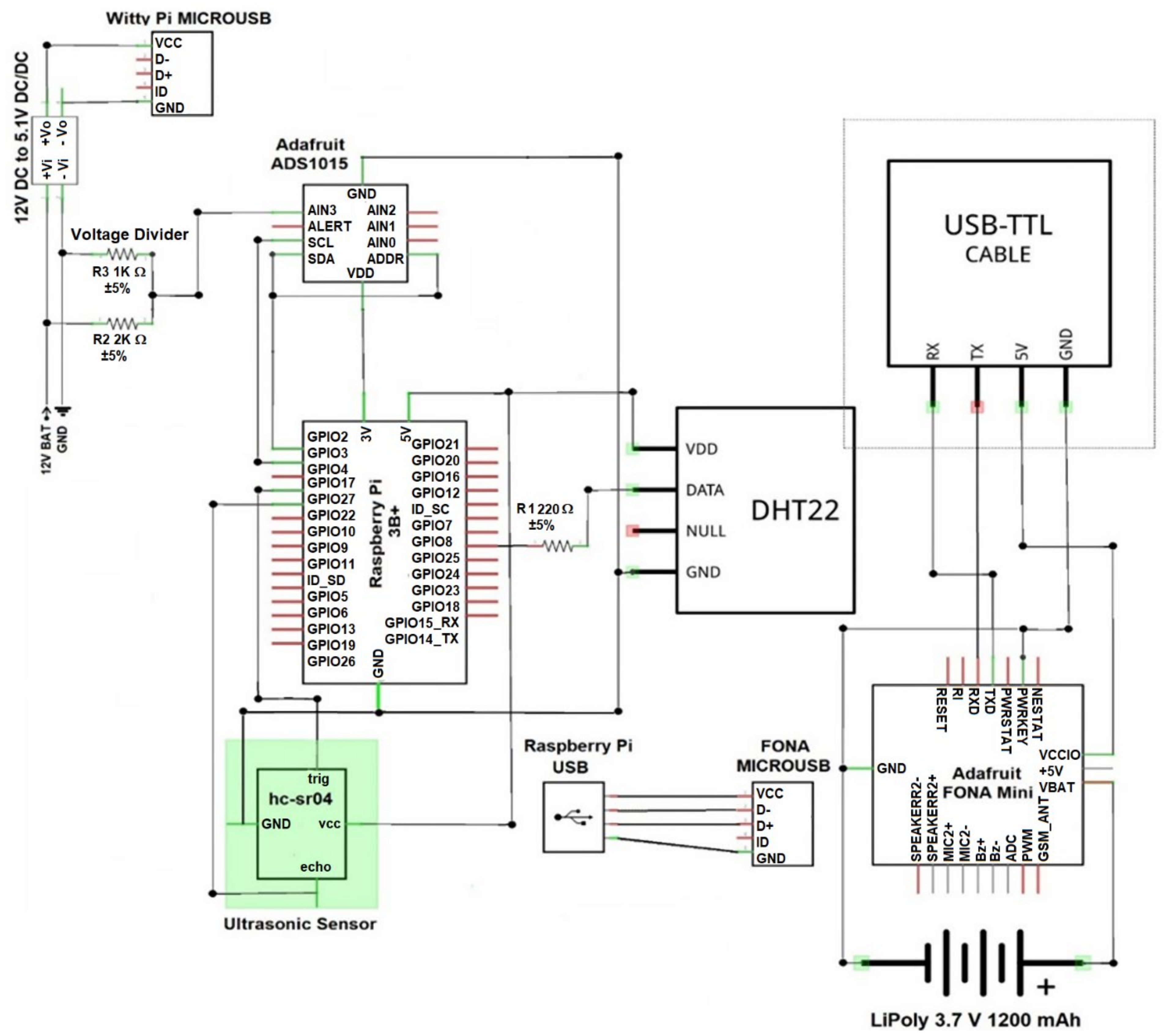
Each system has different types of sensors regarding the variables measured, although they have a general structure (
Figure 1). The sensors described below were selected considering not only their price, but also their behavior in measurement quality and viability (proven in the field); and their accuracy was increased following the up-to-date techniques of measuring and calibration.
2.1.1. Hydrologic Monitoring System
The main objective of the hydrological monitoring system is to monitor a circulating water flow, to measure runoff through channels and riverbeds. It is composed of an ultrasonic sensor hc-sr04 (which uses a sonar, with neither sunlight nor black materials affecting its operation), manufactured by Cytron Technologies Sdn. Bhd (5 to 15 €, reference price for Europe updated in October 2021), to measure water depth (y); it works on a 5 V DC power supply and requires 15 mA of working current, in a measurement range from 2 to 400 cm, an effectual angle <15°, a measured angle of 30°, and has a resolution of 0.3 cm [
41]. Additionally, there is also a DTH-22 Adafruit industries sensor (5 to 10 €), which works within −40 and 80 °C, with an accuracy of ±0.5 °C for air temperature measurements (T), and between 0% and 100%. It has an accuracy of 2–5% for relative humidity (RH) measurements, operating with 5V DC in a 2.5 mA max current [
42] (
Figure 2).
The measurement of y through the ultrasonic sensor is based on the speed of sound, which is affected by air conditions; thus, the methodology described by Wong and Embleton [
43] is used to correct the speed of sound by using T and RH real-time data. Additionally, to avoid water depth fluctuation, since a turbulent flow is expected, y was calculated as an average of several consecutive measurements.
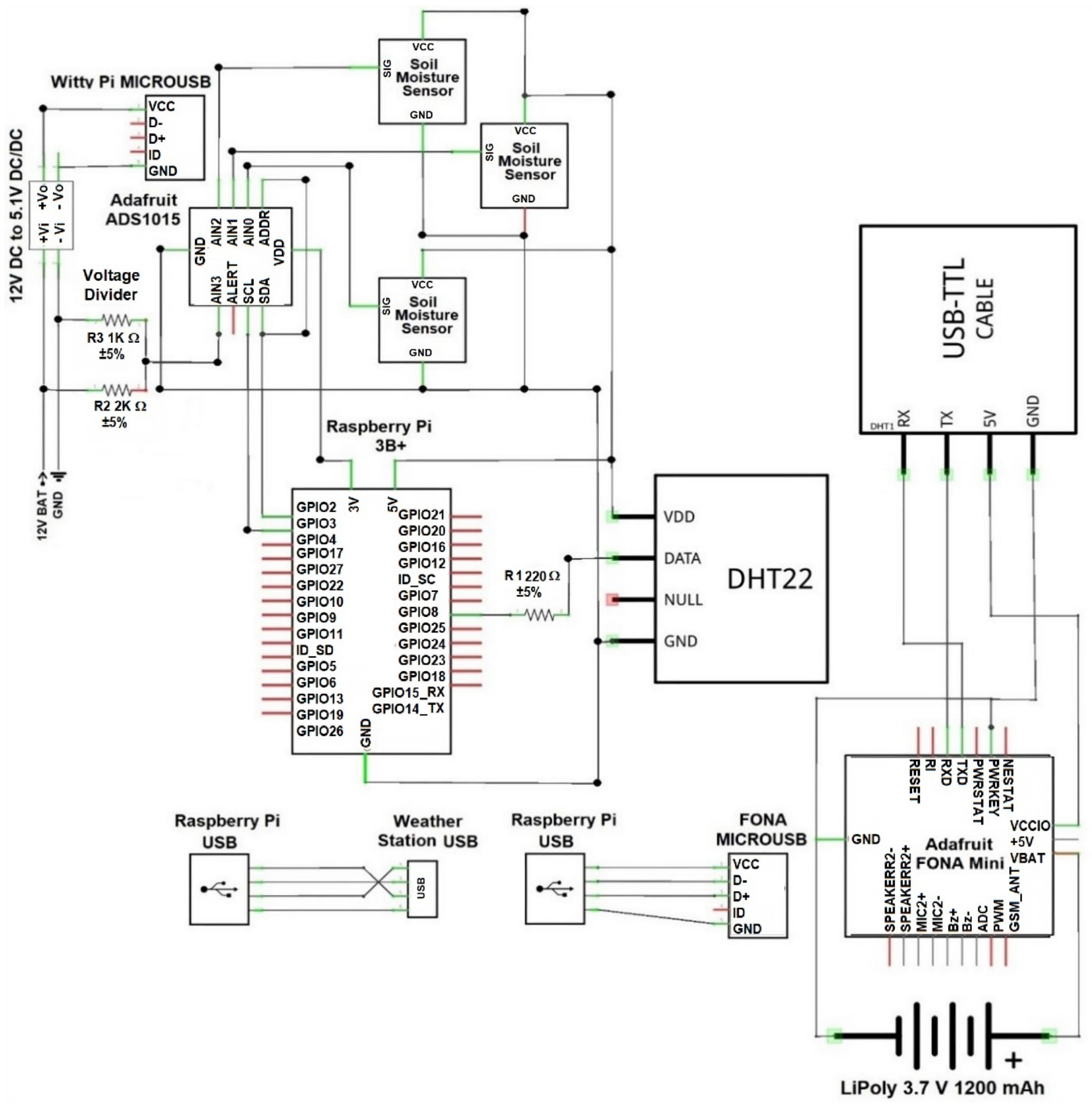
2.1.2. Meteorological Monitoring System
The meteorological monitoring system controls several variables (precipitation, wind speed and direction, soil water content, air temperature, relative humidity, air pressure, etc.), and consequently, it integrates a large number of sensors: a rain gauge, an anemometer, a weathervane, a barometer, a thermometer, a hygrometer, and a soil moisture sensor (
Figure 3).
Most of the sensors in this system are included in the WS1060 (ED31502) Velleman weather station and comprise two segments (80 to 120 €). One segment corresponds to the instrumental part containing the sensors (rain gauge, anemometer, wind vane, thermometer, and hygrometer), and a radio transmission system for transmitting the sensor measurements to the receiver, located in the second segment that includes a microcontroller, a graphical interface, some sensors (thermometer and hygrometer), and a USB port for data management (
Table 1) [
44].
A DHT-22 sensor was also included to monitor interior temperature and humidity, to foresee and identify possible issues, such as overheating or high humidity, which could lead either to the corrosion and/or malfunction of electronic components. In addition, the capacitive anticorrosion sensors (Waterproof Capacitive Soil Moisture Sensors SKU SEN0308, DFRobot; 5 to 10 €) were used to measure soil water content, which is related to frequency domain reflectometry (FDR). They work at 3.3–5.5 V DC with a 5 mA power supply and generate an analogue output range of 0–2.9 V DC [
45].
2.1.3. Common Components
The hydrological and meteorological systems include different sensors, since they measure different variables, although both share common components which complement their operation regarding data logging, data transmission, and power supply.
Microcomputer
The platform is based on a Raspberry pi 3 B+ (35 to 70 €), a single-board microcomputer controlling all the processes (sensor activation, operation, data calibration, interpretation, logging, and transmission). It has a 1.4 GHz 64 bit quadcore processor, 1GB LPDDR2 SDRAM, a dual band (2.4 GHz and 5 GHz) wireless LAN, Bluetooth, four USB 2.0 ports, a 40-pin GPIO header, and a micro SD port, and requires a power input of 5.1 V DC 2.5A [
39].
Real-Time Clock
The Raspberry pi model 3 B+ does not include an internal real-time clock (RTC), so a Witty pi 2 RTC from UUGEAR was implemented (18 to 20 €). It not only allows one to manage time, but also controls Raspberry pi’s ignition and shutdown. It uses an extremely accurate I2C RTC, the DS3231SN, which can count in seconds, minutes, hours, days of the month, months, days of the week, and years, with a leap-year compensation that is valid up to 2100. Its accuracy is ±2 ppm from 0 °C to 40 °C, and it works with a CR2032 or CR2025 battery, consuming 1 mA in standby current [
46].
Data Transmission
Data transmission is driven by GPRS technology—the GPRS/GSM Adafruit cellular FONA Mini (40 to 60 €), a small GSM cellular module powered by the SIM800, and a quad-band (850/900/1800/1900 MHz) module for connecting onto any global GSM network with any 2G SIM card. It makes it possible to send and receive GPRS data through different protocols (TCP/IP, HTTP, etc.), and to send and receive SMS messages, phone calls, and FM radio broadcasts. It operates with AT commands and its circuitry can run from 2.8 V to 5 V DC [
42]. To complete data transmission, a quad-band antenna (3 to 5 €), a 3.7 V DC 1200 mAh Lipoly Battery (5 to 10 €), a USB- TTL serial cable, and a USB to micro-USB cable are also required (both: 8 to 15 €).
Data Logging
In addition to the wireless data transmission and its subsequent cloud storage, and as a security backup, an SQLite 3 [
47] database was developed for data logging in a 16 GB micro-SD card (4 to 10 €). It creates a data backup within the equipment that can be easily downloaded when data transmission is affected due to possible incidents, such as connection problems, loss of data during transmission, and low or null connection to the GPRS network. Data can be downloaded directly in the field by using a USB cable or a remote access protocol.
Analog to Digital Converter
Since FDR sensors generate an analogic output that cannot be directly connected to the Raspberry pi 3B+ GPIO digital pins, a high-precision analogue to digital converter (ADC), the ADS1015 from Adafruit (5 to 10 €), was implemented. It provides 12-bit precision, at 3300 samples per second, over I2C, and can be configured as 4 single-ended input channels or two differential channels. It includes a programmable gain amplifier, up to x16, to help boost smaller signals to the full range. This ADC runs on 2 to 5 V power, and has low current consumption (150 µA) in continuous mode [
42].
Power Supply
The Raspberry pi microcomputer requires a 5.1 V DC and 2.5 A power supply for proper operation (a lower or higher power supply can cause corruption of the microSD card, erratic behavior, and hardware damage). In the case of direct access to AC power supply network, the equipment can be powered directly through a charger; however, for field installations, a photovoltaic electrical supply system must be used. In this case, a 12 V 50 W monocrystalline solar panel was integrated (50 to 80 €), with a 12 V 14 A rechargeable battery (20 to 40 €), a charge controller (10 to 20 €), and a DC-DC voltage reducer (LM2596; 8 to 15 €); these elements can provide energy for the normal operation of the system with autonomy for 3 days in the season of least solar incidence regarding the power consumption of the equipment.
In order to reduce power consumption, the system will enter hibernation mode once it has measured and transmitted data. In addition, a voltage divider was incorporated, which reduced the battery voltage from 12 V to 4 V. It sends this output to one of the ADC’s analogue ports to monitor battery status.
2.1.4. Web Platform
The data logged in the equipment are transmitted to an Internet of Things (IoT) Web platform for further interpretation. In this study, a cloud-native platform, Altair SmartCore, which allows one to manage up to 10 different devices for free, was used [
48].
2.1.5. Runoff Model
Six different models were studied to predict peak runoff: the rational method (Equation (1)), the NRCS-TR55 (Equation (2)) [
49], Espey (Equation (3)) [
50], the modified rational method (Equation (4)) [
51], the Spanish standard 5.2-IC for highway drainage design (Equation (5)), and the NRCS triangular hydrograph [
49]
where
Qp stands for the peak flow,
I for the rainfall intensity,
ci for the runoff coefficient,
A for the area, and
i for each land use within the catchment.
where
qu represents unitary flow and
Fp is a pond and swamp adjustment factor.
where
tp is the peak time,
tb is the time base, and
k is a correction factor.
To estimate the time of concentration (
tc), we use three different equations: kirpich (Equation (6)) [
52], the Spanish standard 5.2-IC for highways drainage design (Equation (7)), and the Bransby–Williams method (Equation (8)).
where
L is the riverbed length and
J is the average gradient.
2.2. Control Logic and Communication
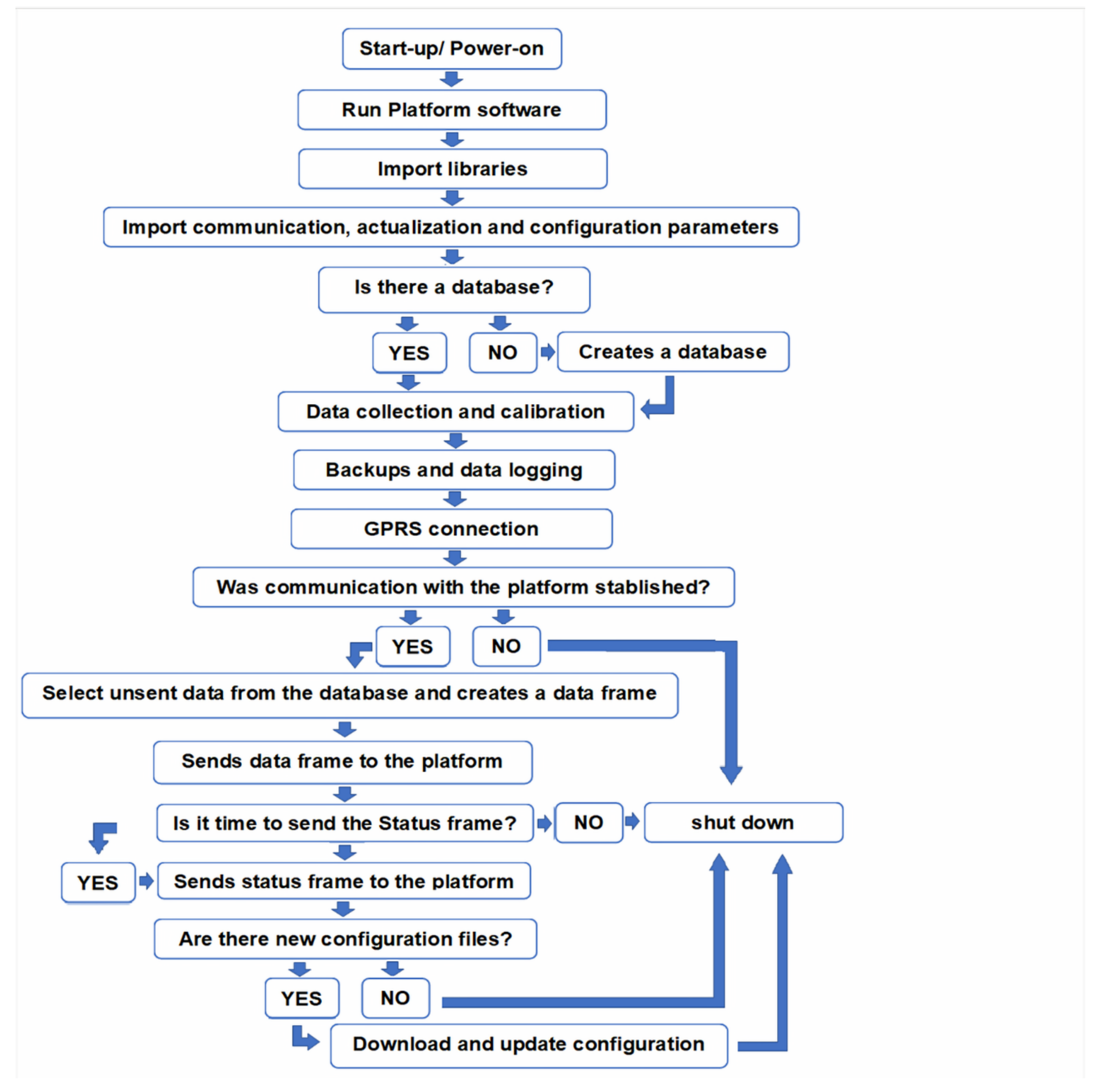
The software developed to control the platform was written in Python 3, an interpreted, high-level, general-purpose, and open-access programming language [
40]. It runs automatically after the equipment’s startup. It first loads the initial parameters and libraries. Then it verifies the existence of a database (if there is no database, it creates one), reads the sensors, calibrates the data to ensure the highest precision and accuracy, stores the data within the database, establishes communication with the Web platform through the GPRS module, and transmits the data not previously sent (
Figure 4).
If communication with the Web platform fails (e.g., no GPRS connection), the equipment will shut down and wait for the next cycle; thus, it will avoid unnecessary power and mobile data consumption associated with frequent retries. Nevertheless, if communication is successful, data will be sent grouped into two types of frames: a data frame (integrated by the data measured by the different sensors) and a status frame (sending parameters regarding the devices status). So as not to resend data, an identifier is incorporated into each frame successfully sent, so that next time they will not be considered. Furthermore, to avoid problems with the massive sending of frames, which can cause a failure in communication, the maximum number of frames sent at the same time is limited.
In addition, two configuration files were also developed to remotely change certain variables and the equipment’s operation and communication protocols: a connection configuration file (cc, including Web platform connection parameters) and a general porpoise configuration file (cg, allowing the modification of some operating parameters). Therefore, once the frames are successfully sent to the Web platform, the program will verify if there are modifications in the configuration files. In case of a change in any of the parameters from the configuration files, the equipment will download and update them; if not, the equipment will directly shutdown. The computer code developed in this study is openly available in a GitHub repository:
https://github.com/dasegovia/hydromonitoring-system.git (accessed on 10 September 2021).
2.3. Field Assessment
The “Venero Claro” basin (15.53 km
2), located at the eastern Sierra de Gredos in Central Spain, was selected as the pilot emplacement of the monitored platform (one of each monitoring system was installed on the basin). This is because it has been extensively monitored (nowadays it has Davis rain collector tipping bucket rain gauges and one Seba radar water level sensor in six locations,
Figure 5) due to its torrential water behavior. Topography, elevation, rugged relief, and north orientation combine to generate strong rainfall events, high runoff, and flash floods [
53].
The meteorological monitoring system was located in a central area of the basin at 40°23′45.5″ latitude N, 4°39′06.5″ longitude W, and 896 m a.s.l.; and the hydrologic monitoring system at 40°24′18.3″ latitude N, 4°39′39.2″ longitude W, and 776 m a.s.l. The latter was mounted under a bridge near the mouth of the main channel, not only to take advantage of the infrastructure as support for the equipment, but also because it has a known rectangular and an invariable concrete section, which facilitates hydraulic calculations, and because the radar water level sensor is also located in this place.
Since the water level sensor measures the distance from it to the channel bed, water depth must be calculated as the difference between the sensor measurement (x) and the distance from the sensor to the base of the channel (h). In this case, the sensor was mounted at 364 ± 1 cm from the channel bed.
The water flow (
Q) was estimated as a function of
y by Equation (9), obtained by Puig (2018) [
54], using the IBER software in the section under the bridge.
Both monitoring systems were installed following the guidelines of the WMO No.49 technical regulations [
38] in June 2019. Additionally, the emplacement was determined according to the methodology described by Zubelzu et al. [
55].
2.4. Calibration and Validation
The rain gauge, the water depth sensor, and the FDR soil moisture sensors, whose measurements of basic variables were uploaded to the runoff model, were tested, calibrated, and validated in the laboratory, as described below.
2.4.1. Water Depth Sensor
The ultrasonic equipment was mounted above the water surface storage in a water tank with a scale (0.1 cm resolution) for the water level measurement; the measurements of both the water tank scale and the sensor were contrasted through the coefficient of determination (R2) and a root mean square error (RMSE). Fifty different water depths were tested between 7 to 200 cm, and six repetitions for each depth were run within a 5-min interval. The sensor was installed 250 cm above the bottom of the tank.
2.4.2. FDR Soil Water Sensors
For the calibration of FDR probes, two different soil samples from the Venero Claro mountain basin were chosen; one was taken at the A horizon, within a depth of 15 cm, with sandy loam texture, and the other at the B horizon, within the interval of 15 to 37 cm depth, with sandy texture. The bulk density of each soil was determined by the core method.
Seven different soil moisture contents (θ) determined by the volumetric method were tested for each soil (from dry to saturation). The soil samples were oven dried, at 105 °C for 24 h, and then they were carefully placed in seven 2 l plant pot containers for each soil (one for each θ), to maintain the soil’s bulk density. The procedure consisted of adding a given water volume to each container, which was distributed homogeneously in the soil by mixing, for each θ tested level except for the dry (no water was added) and saturated soil (obtained by capillarity). Finally, the real soil moisture contents were determined by the gravimetric method, weighing samples extracted from each soil moisture tested level in a precision laboratory balance (resolution = 1 mg) with the common assumption that 1 g is equivalent to 1 cm3 of water, before drying it to obtain θ by the difference between dry and wet weight.
Six repetitions were performed for each θ and soil type, in four FDR sensors, where five were used for calibration and one sample was used for validation, through R2, RMSE, and mean absolute error (MAE). Thus, the total number of measurements was 336, and 56 were used for validation.
2.4.3. Rain Gauge
Rain gauge was calibrated in the laboratory, at first, via static calibration as in [
56]; then, dynamic calibration by simple nonlinear regression according to the UNE-EN 17277:2021 Spanish standard was performed.
During static calibration, water was added, drop by drop, reaching an accuracy of 0.1 mm per tip on both rain gauge buckets. Then, a constant-head siphon connected to a nozzle, similar to the one used by Sypka [
57], was used to keep a steady flow rate in a 30 min test for each tested rainfall intensity measured by a 0.01 s resolution chronometer. The volume of water used on each test was measured by weighing it in a 1 mg resolution precision laboratory balance, assuming 1 g = 1 cm
3.
A total number of 80 tests were performed at different rainfall intensities, up to a maximum of 400 mm·h−1. Of these, 45 were used to calibrate the sensor and 35 for validation by R2 and RMSE.
2.4.4. Runoff Model
Four real storms that occurred in the Venero Claro mountain basin were studied to define which of the six proposed runoff models best fits in with reality (
Table 2), through an RMSE.
3. Results and Discussion
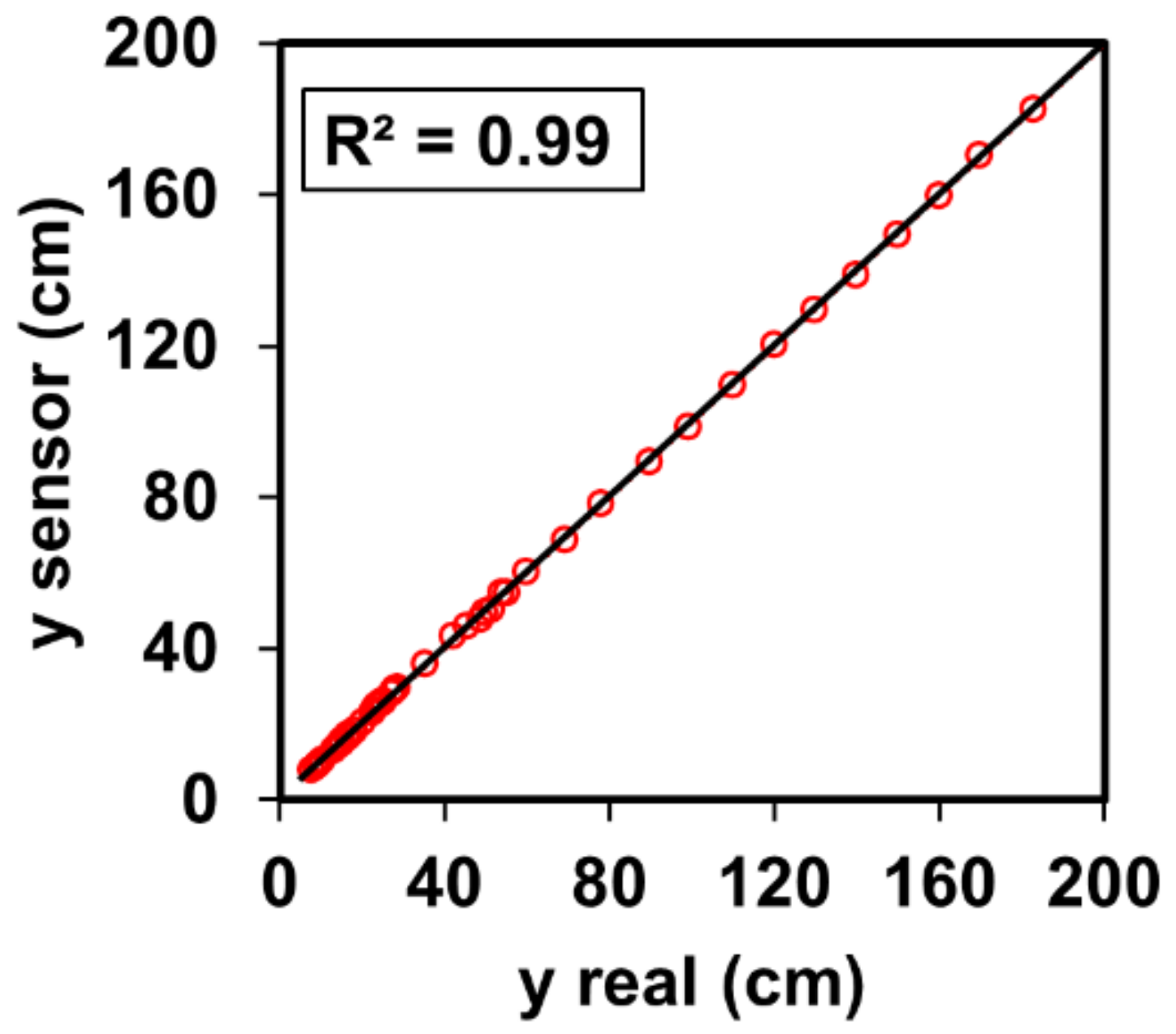
3.1. Water Depth Sensor
With laboratory calibration, we obtained a coefficient of determination between sensor measured values and the real water level of R
2 = 0.99 (
Figure 6). The mean absolute error was ±0.51 cm, the relative error was 1.65%, the RMSE was 0.41 cm, and the maximum absolute error between repetitions was ±1.39 cm.
3.2. Soil Moisture FDR Sensors
In dry soil, the four FDR studied sensors output zero. The subsequently measured moisture levels were agreed upon fairly well by the sensors, and the same behavior was found. A sigmoid function, with an R
2 = 0.97 for both soils, sandy loam and sandy, was observed (
Figure 7).
The voltages returned by the sensors between repetitions, and even between different sensors, presented some variability. The voltage was higher at low moisture levels and decreased as θ increased. The sensors are less sensitive near saturation than in dry soils; thus, at high θ, a small change in sensor voltage causes a larger jump than at lower θ.
The coefficients of variation (
CV) between sensors and among tests were similar; the variations among manufacturers appear to be small compared to the variations among measurements, which makes it possible to apply a single calibration procedure (depending on the soil type) to all sensors (
Table 3). This variation could be caused either by the actual soil variability and/or the non-uniformity of
θ distribution within the sample.
The
CV was higher at the lower
θ within the humidity interval and decreased as
θ increased. This performance could be caused by poor sensitivity to changes when dealing with high
θ values (see
Figure 7a); nevertheless, the measurement errors were amplified despite the smaller
CV due to the sensitivity loss in the sensors (
Table 3). The R
2 results were: 0.98 and 0.99 for the sandy loam and sandy soil, respectively (
Figure 7b). Sandy loam soil presented larger RMSE (15.32%) and MAE (±2.2%) than sandy soil (1.87% and ±0.93%, respectively); smaller error values may have been due to the more homogeneous composition of the sandy soil.
Figure 7b and
Table 3 show that at the two highest
θ levels studied, the sandy loam soil presents the largest error increment, and an outlier is observed coinciding with the penultimate
θ level (field capacity), which was identified by the sensor as saturated soil. This outlier could be caused by several factors, such as soil
θ variation, loss of sensitivity in the sensor, and/or an experimental error. Nevertheless, a high precision at
θ, over the field capacity interval, is not required, since any value beyond this can be considered saturated soil. In this case, if only
θ values up to field capacity are considered, the errors drop drastically to 2.05% and to 0.82% in RMSE and to ±1% and ±0.67% in MAE for the sandy loam and sandy soil, respectively.
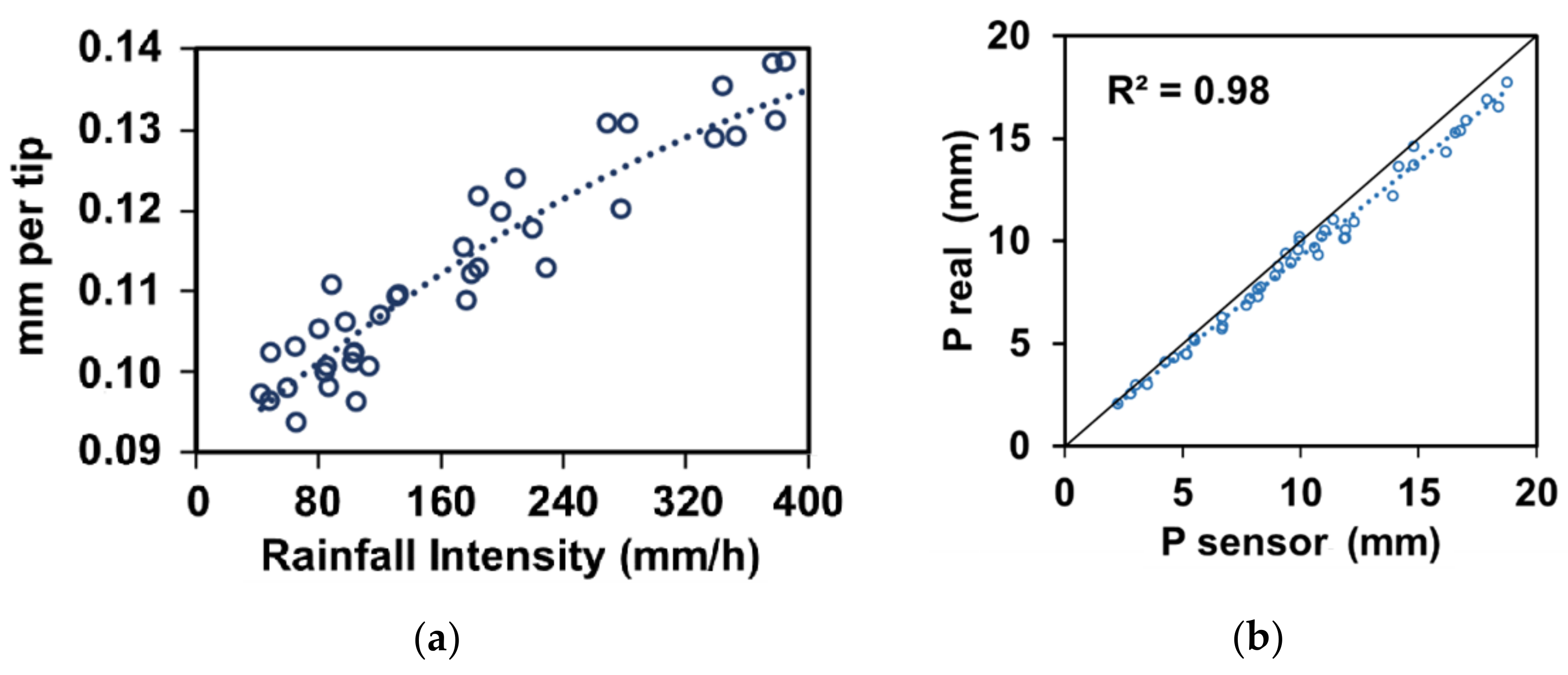
3.3. Rain Gauge
The volume needed for tipping increases as precipitation intensity increases when fitting a polynomial regression with an R
2 = 0.94, as was expected according to the UNE-EN 17277:2021 Spanish standard (
Figure 8a). In validation, a R
2 = 0.98, an RMSE of 0.87, and a mean absolute error of ± 1 mm were obtained (
Figure 8b).
3.4. Cost Analysis
One complete hydrologic monitoring system can have a hardware cost of 216 to 380 €, and a complete meteorological monitoring system—296 to 495 €. A traditional weather station with similar characteristics, including solar power supply and GPRS data transmission, can have a cost of 500 to 1300 €, and a conventional water depth monitoring system may involve a cost of 500 to 1200 €. However, conventional monitoring systems have an extra cost due to data transmission, logging, and Web platform user access; in our case, we use a free Web platform (for up to ten devices) and the IoT SIM card has a cost of 3 € per month. These prices were consulted in October 2021 in different locations and sales Web pages in Europe; prices vary from site to site.
The main disadvantage of low-cost monitoring projects is the design, especially the software design, but in this case, platform design and software are freely available and can be easily optimized or adapted for different monitoring projects.
The solar panel supply system and the transmission module are the most expensive components in the platform, with costs of 88 to 155 and 56 to 90 €, respectively.
3.5. Field Implementation and Data Collection
Since June 2019, the monitoring systems have been sending data discontinuously; the measurements have been logged every 10 min (the same frequency used for data frame transmission), and an 8-h transmission was settled for the status frames, although these frequencies changed in some cases to test the system’s updating capacity.
During this period, some problems arose, mainly related to the loss of mobile coverage and power supply, due to inconveniences of biotic (rodents, ants, bees, etc.) and abiotic nature (e.g., high temperatures), which generated lapses without data. However, these problems were solved, making it possible to identify bugs in the protocols and generate a more robust system and platform, which are currently working satisfactorily.
3.5.1. Hydrologic Monitoring System
The main problem present in this system was the loss of GPRS coverage due to its location in a natural canyon, surrounded by stone and the concrete walls of the bridge structure. However, it has been possible to obtain data of y and the other variables due to the protocol implemented in the device to solve data transmission problems and the data backup, which allows field access to data, as described by Hund et al. [
4].
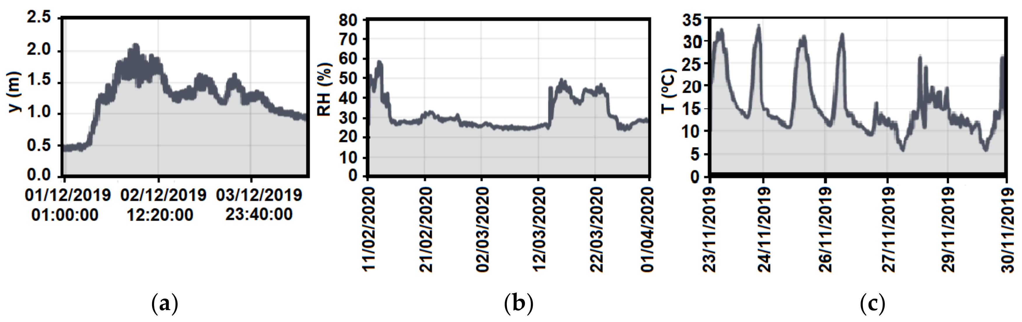
The hydrological year during the field implementation was a dry year, which led to most of the data being collected from a dry bed. However, in
Figure 9 a storm that occurred in December 2019 is presented as an example. The variation in water depth is noticeable.
3.5.2. Meteorological Monitoring System
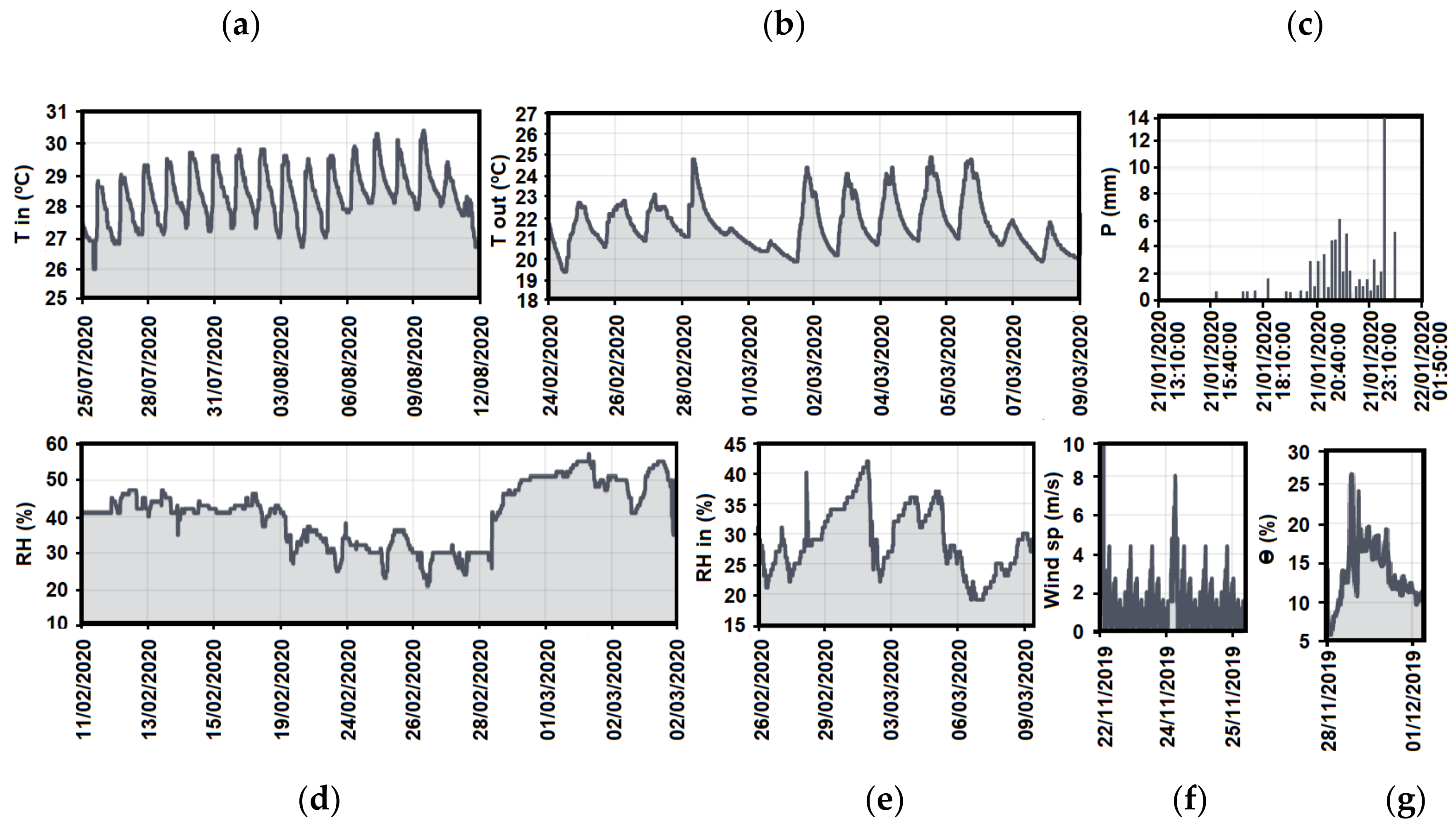
In this monitoring system, data transition was not an important problem, since the low mobile coverage had a greater impact on the hydrologic system, probably due to its location. However, the main problems presented in this system were due to the power supply, but they were easily overcome.
Figure 10 shows the variations in the daily air temperature and relative humidity, logged precipitation data during a storm, and other information. The sensors performed similarly to traditional commercial sensors, so—as demonstrated by Islam et al. [
23] in their inexpensive real-time hydrological monitoring station—low cost sensors can be used efficiently for hydrological monitoring.
3.6. Runoff Model
According to the RMSE analysis, the NRCS models [
49] fit in better with real measured data, the NRCS-TR55 being the best in T1 and T2, and the NRCS triangular hydrograph being the best in T3 and T4. The Spanish standard 5.2-IC for highways drainage design and the Bransby Williams equations for
tc are those that obtained the lowest error level (the same error in both;
Table 4).
According to those results, we were able to run different runoff models on the platform with the field data. We obtained promising results, especially for T2 and T4, for which RMSE were below 1. However, values in T3 and especially in T1 are larger, T1 being the storm with the largest Qp. Therefore, we can say that the low-cost, open-hardware platform proposed for hydrological monitoring has great potential for hydrological monitoring and flood risk management. Being cheaper than traditional commercial alternatives, it opens the door to the development of a new generation of hydrological monitoring networks. Nevertheless, it requires a properly selected runoff model.
4. Discussion
The results highlight that, with proper sensor programming and calibration, a low-cost ultrasonic sensor can be efficiently used to monitor water level fluctuations, as previously demonstrated by Prima et al. [
58]. The need for a rapid response in flood risk management has motivated the accelerated development of WSNs in this area [
3], and several studies report the use of low-cost ultrasonic sensors for different purposes (monitoring diesel levels in fuel tanks, water level in cisterns, etc.) and to provide real time river stage information in flood risk management systems [
1,
27,
32,
36]. Likewise, wireless networks of low-cost sensors are suitable for early flood warning systems, deployed at much larger spatial scales at affordable prices [
3].
In many areas, the systems devoted to water resources and flood risk management play a key role in the accurate monitoring of water levels, at high spatial and temporal scales [
3,
27]. Thus, low-cost ultrasonic sensors have the potential to serve as viable alternatives for water depth monitoring.
Soil water content is recognized as one of the main drivers for the plant ecosystem and an important state variable for hydrological modelling. It is characterized by strong spatial variability caused by the variability of soil properties and landscape characteristics; these behave differently when the catchment is upscaled. Thus, the processes controlled by soil’s water dynamics, such as the transport of solutes at the catchment scale and plant ecosystem dynamics, show considerable uncertainty. In addition, soil water monitoring at the basin scale is essential in many hydrologic and agricultural applications [
1,
59]. The results have proved that FDR sensors are an effective alternative for monitoring
θ, and due to their low cost, they are feasible for an extensive monitoring network, as was suggested by Majone et al. and Bogena et al. [
28,
59].
According to Bogena et al. [
28], the sensitivity of the sensor’s reading of soil water content decreased strongly with increasing soil water content. This was also observed in our results, where the voltage returned by the sensors presented variability that was higher at low moisture and decreased as
θ increased. Since the sensors are less sensitive near saturation than in dry soils, at high
θ, measurement errors amplify due to the sensitivity loss in the sensors.
Variation among repetitions was larger than between different sensors, due to soil variability. FDR sensors are sensitive to variations of temperature [
28], so proper calibration depending on the soil is needed to reduce error, as recommended by Majone et al. [
57]. However, variations among different sensors were relatively small. The results have shown that, with proper calibration, tipping bucket rain gauges are an efficient, low-cost alternative for rainfall monitoring, obtaining a minimum error of ±1 mm—even less error than some traditional tipping bucket rain gauges [
37,
56,
57]. Thus, the error levels obtained by these three main sensors allow us to say that the low-cost, open-hardware platform for hydrological monitoring designed in this work is an interesting and promising option for low-cost hydrological monitoring, since the error levels are similar to those reported by traditional monitoring sensors. Nevertheless, the success of the platform is based on proper calibration and sensor programing.
The platform has also proved to be suitable for real implementations and for frequent data transmission to a Web platform; and the runoff model has been executed satisfactorily. Obviously, there are limitations, mainly due to the bad quality of the mobile coverage in the pilot emplacement, resulting from its remote condition, as commonly observed in mountain basins. Nevertheless, it can be improved through other wireless transmission technologies, such as Zigbee digital radios and others that have proven to serve as efficient alternatives in remote places [
1,
2,
34,
60], or even better, through a combination of ZigBee and GPRS technologies, as proposed by Han et al. [
2].
As was demonstrated by Trubilowicz et al. [
26], a wireless monitoring network based on low-cost technologies has great potential for monitoring a great number of variables in real-time hydrological monitoring. However, there are still difficulties to overcome, especially regarding the hardware’s protection from external agents, but low-cost hydrologic monitoring is suitable and can provide a solution to the needs of real-time and high spatial frequency data in flood risk management [
3,
5].
5. Conclusions and Future Directions
The in-field designing and implementation of a low-cost, open-hardware platform for real-time hydrological monitoring, data recording, logging, and wireless transmission has been proposed in this work. The paper described the platform’s performance, the system’s structural design, the hardware implementation, and the software development. Moreover, the calibration of the main sensors in the laboratory improved the accuracy, allowing results as good as in traditional monitoring sensors. In addition, different runoff models were tested to validate the operation of the platform.
The platform has been validated in the field, and the results show that its performance in the measurement, storage, and transmission of hydrological and meteorological data is good; in addition, it includes a remote-control function that, among other features, saves energy and improves its operation. Furthermore, it sends data to an IoT platform, which makes the data accessible at any place and any time with an internet connection.
This open-hardware platform proposed for hydrological monitoring has potential for hydrological monitoring and flood risk management at a lower cost than traditional commercial alternatives; furthermore, it opens the door to the development of a new generation of hydrological monitoring networks and highlights the importance of proper calibration and sensor programing to achieve good results.
The materials presented in this paper may be used as a guide for the development of low-cost monitoring systems for real-time hydrological management. The platform was presented and can be easily modified to incorporate other sensors than those in the paper. Even the IoT platform can be changed and optimized according to one’s requirements.
Future works are expected to include the testing of different sensors on the platform, and the combination of ZigBee and GPRS for data transmission in remote areas; the former is a low-rate radio network suitable for high-level communication protocols used to create personal area networks with a small, low-power digital radio. The Zigbee radio network will transmit data from node to node to an end node, where the GPRS module will transmit data to the Web platform. This will help to evaluate the versatility of the platform, and measured data will be used to evaluate the long-term performance of the efficiency and stability of the platform, but also to develop a runoff model adapted to the pilot basin for flood prevention and flood alert.


