
Modeling of Groundwater Potential Using Cloud Computing Platform: A Case Study from Nineveh Plain, Northern Iraq

 ,
, 
 ,
,  ,
, 
Abstract
:
1. Introduction
2. Materials and Methods
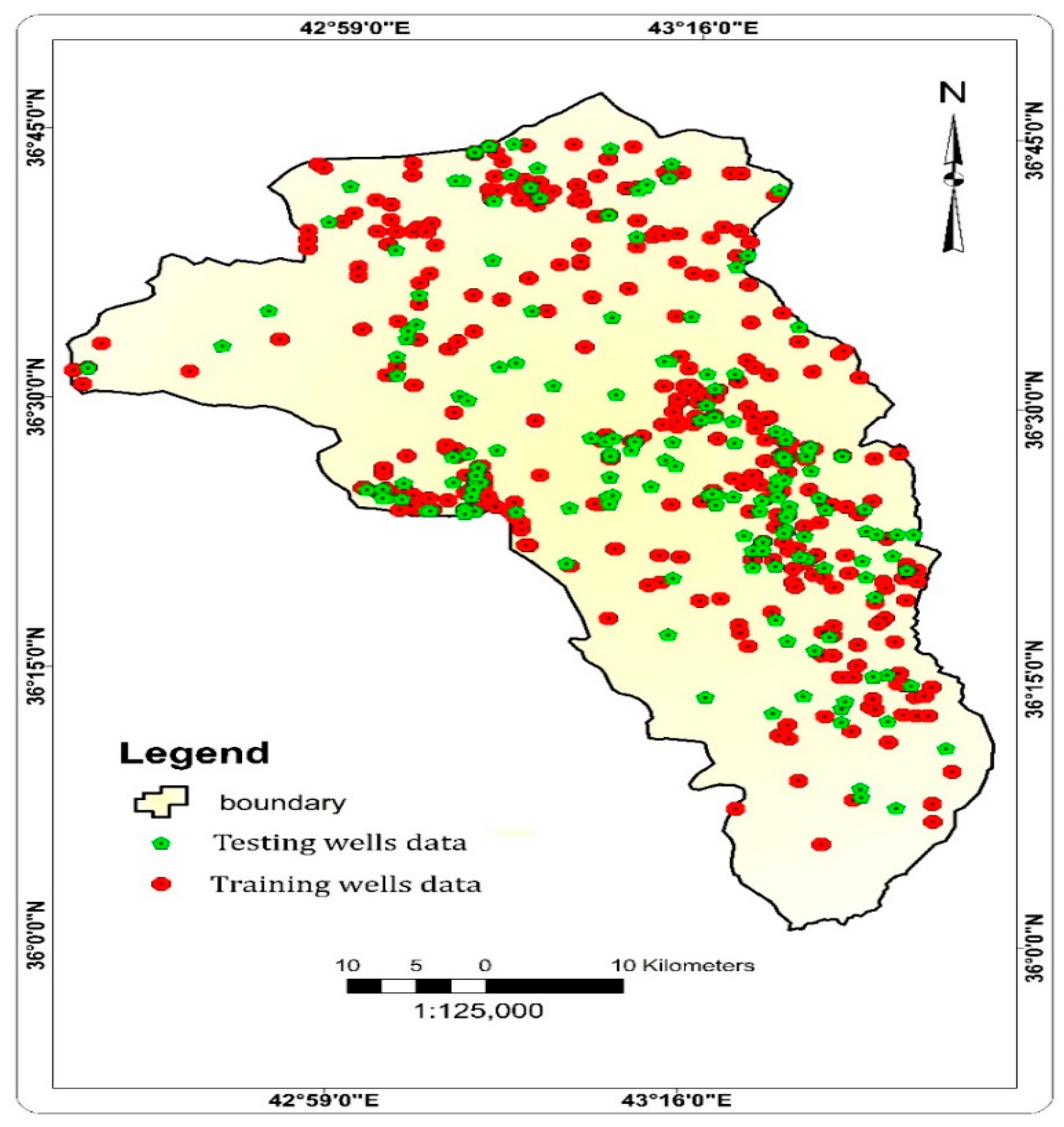
2.1. The Study Area
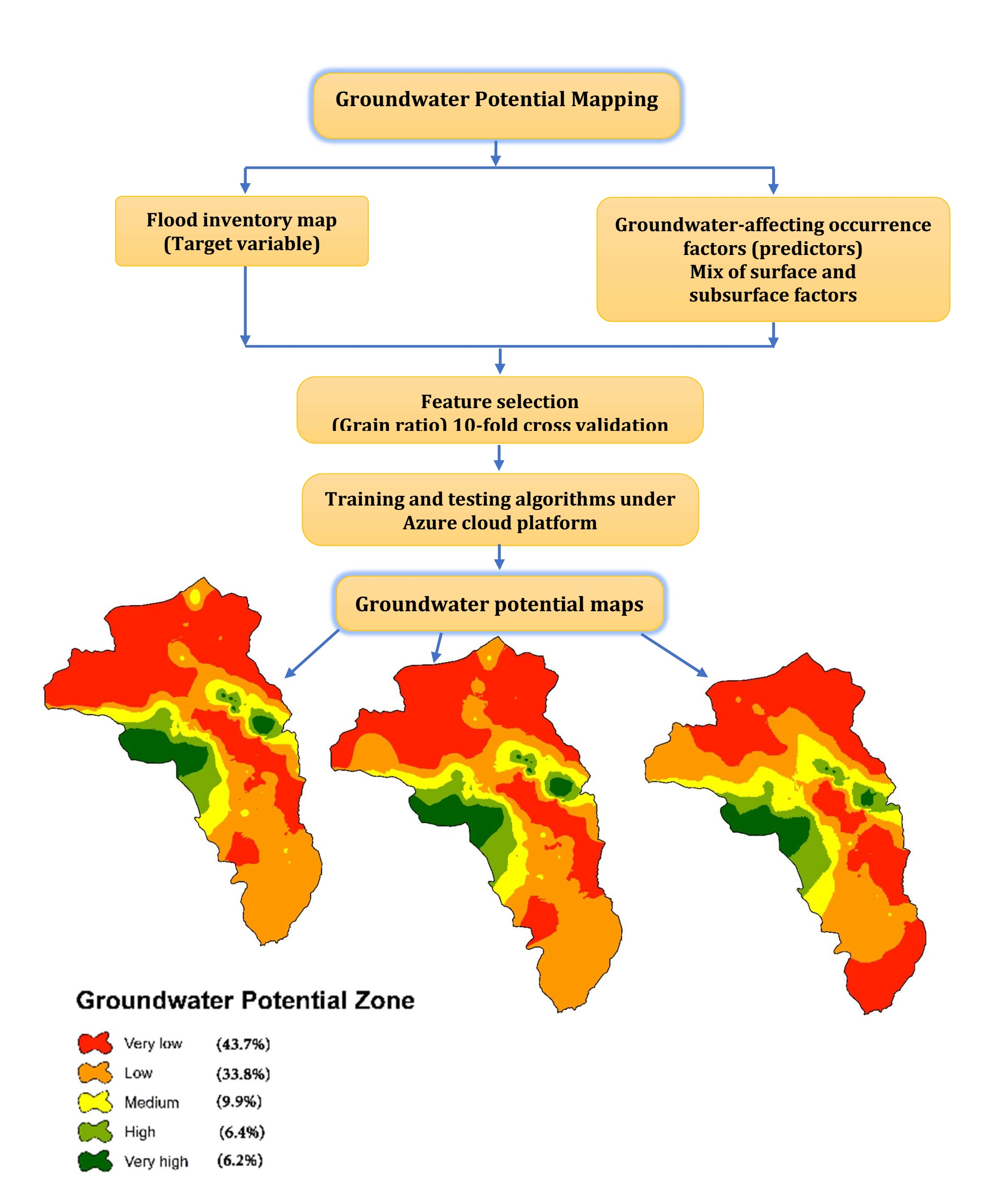
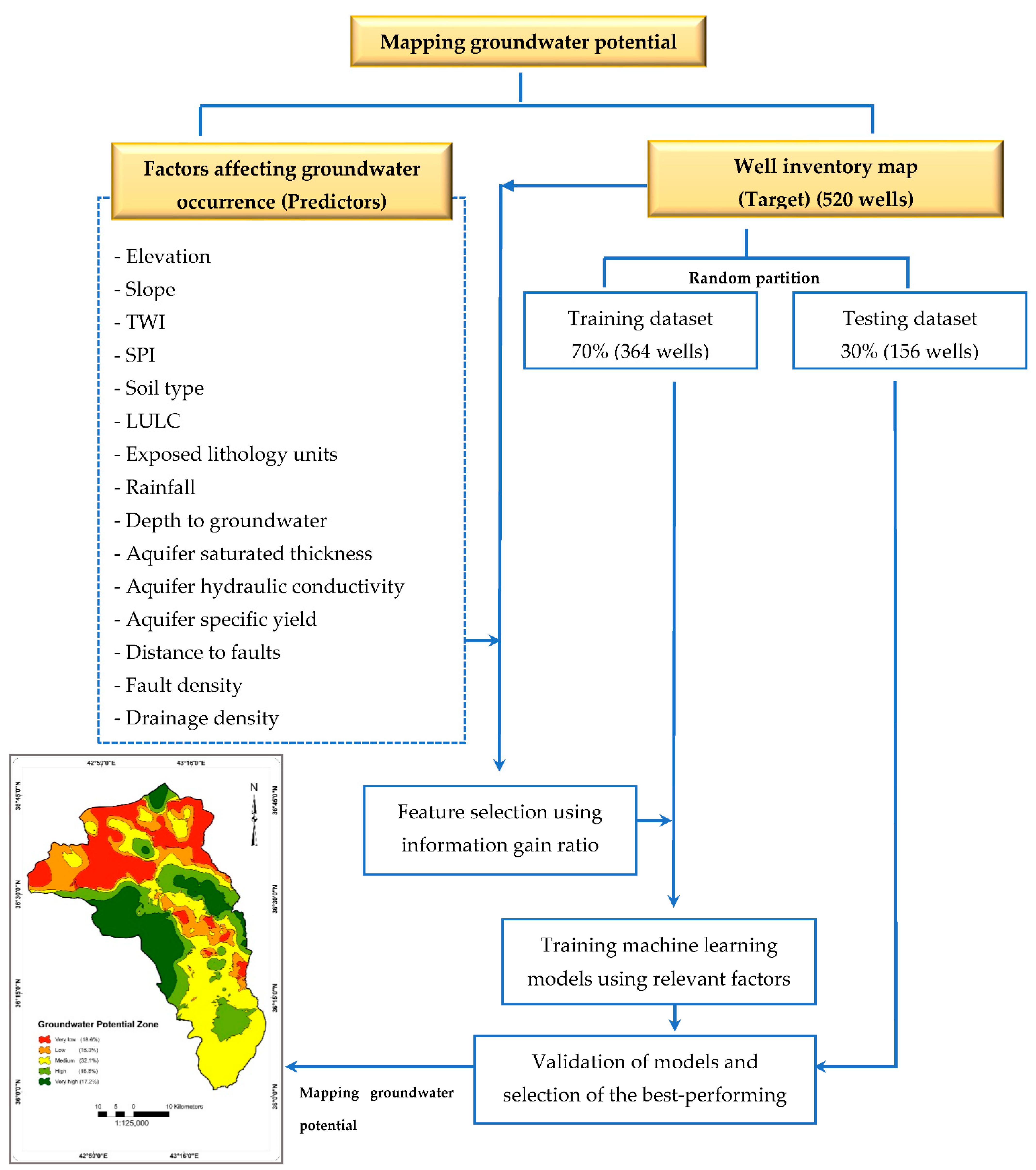
2.2. Workflow Steps
2.2.1. Operating Wells Inventory Map
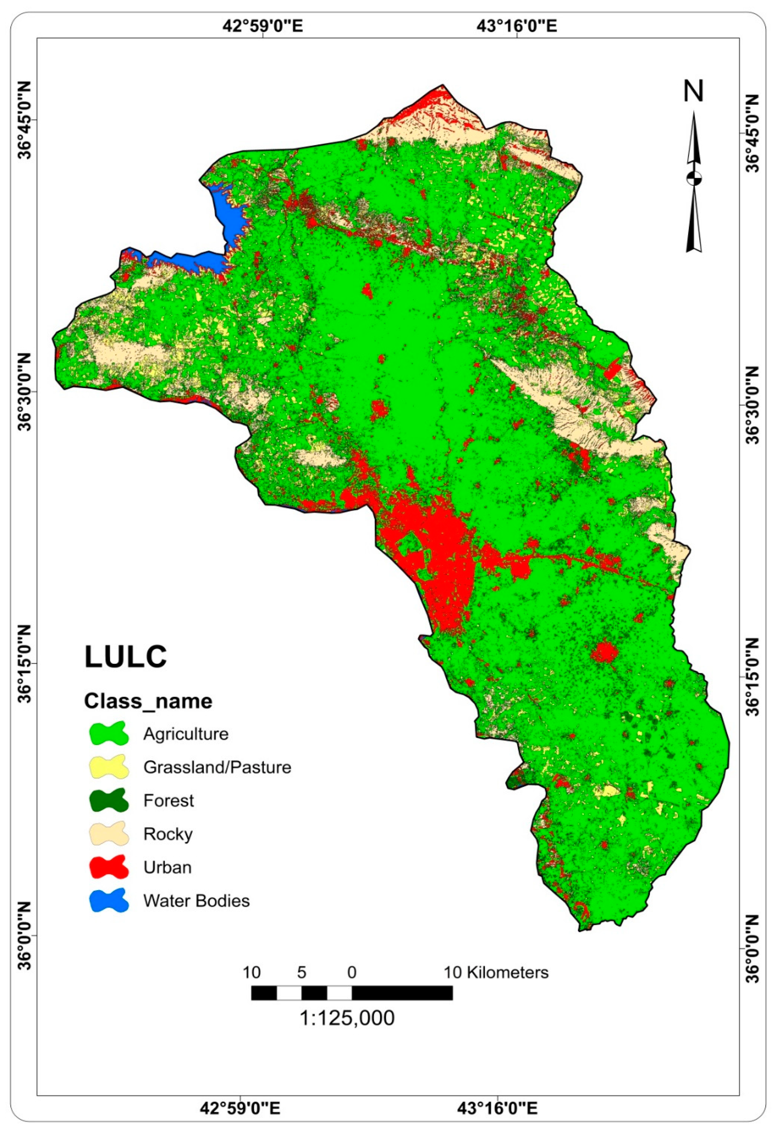
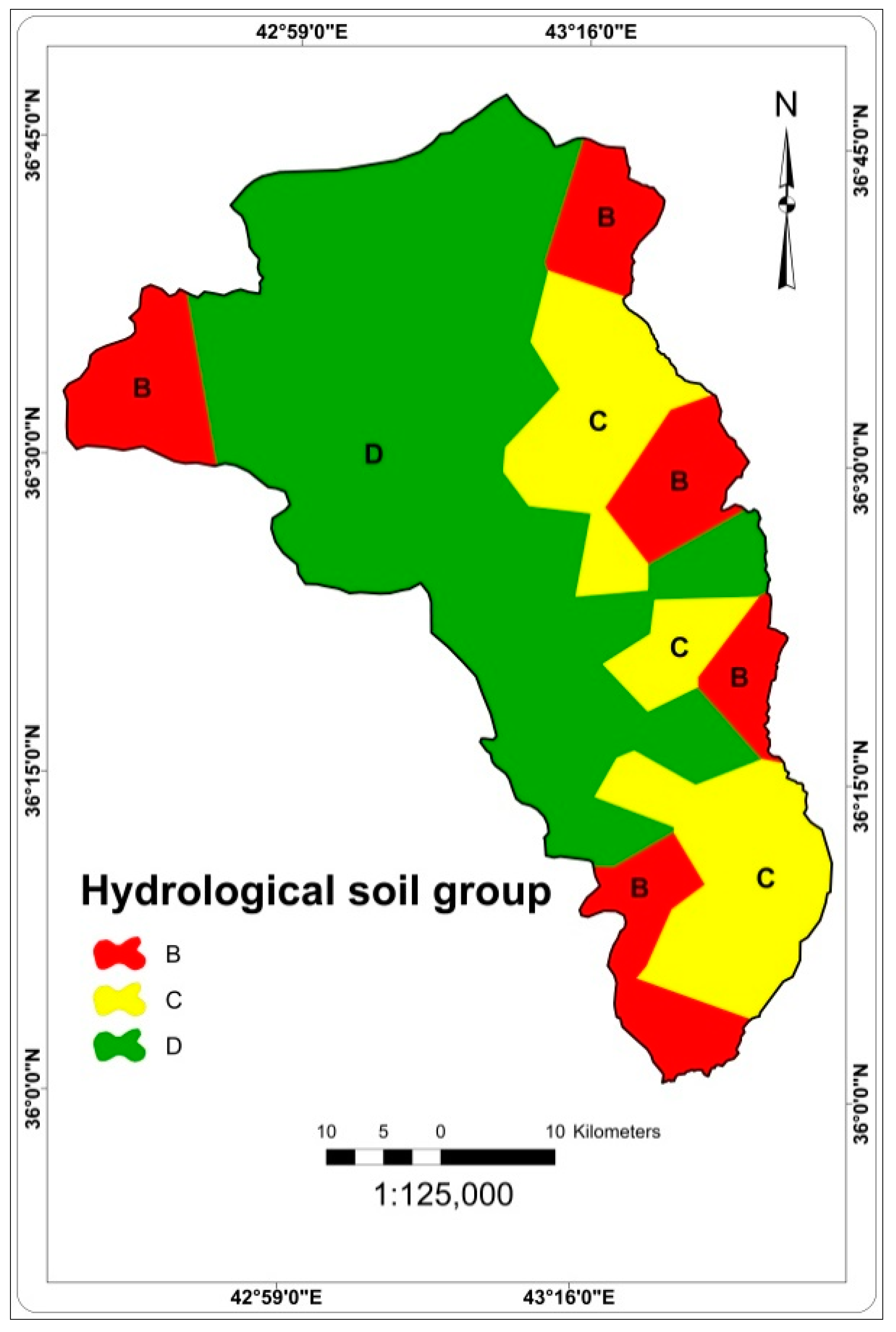
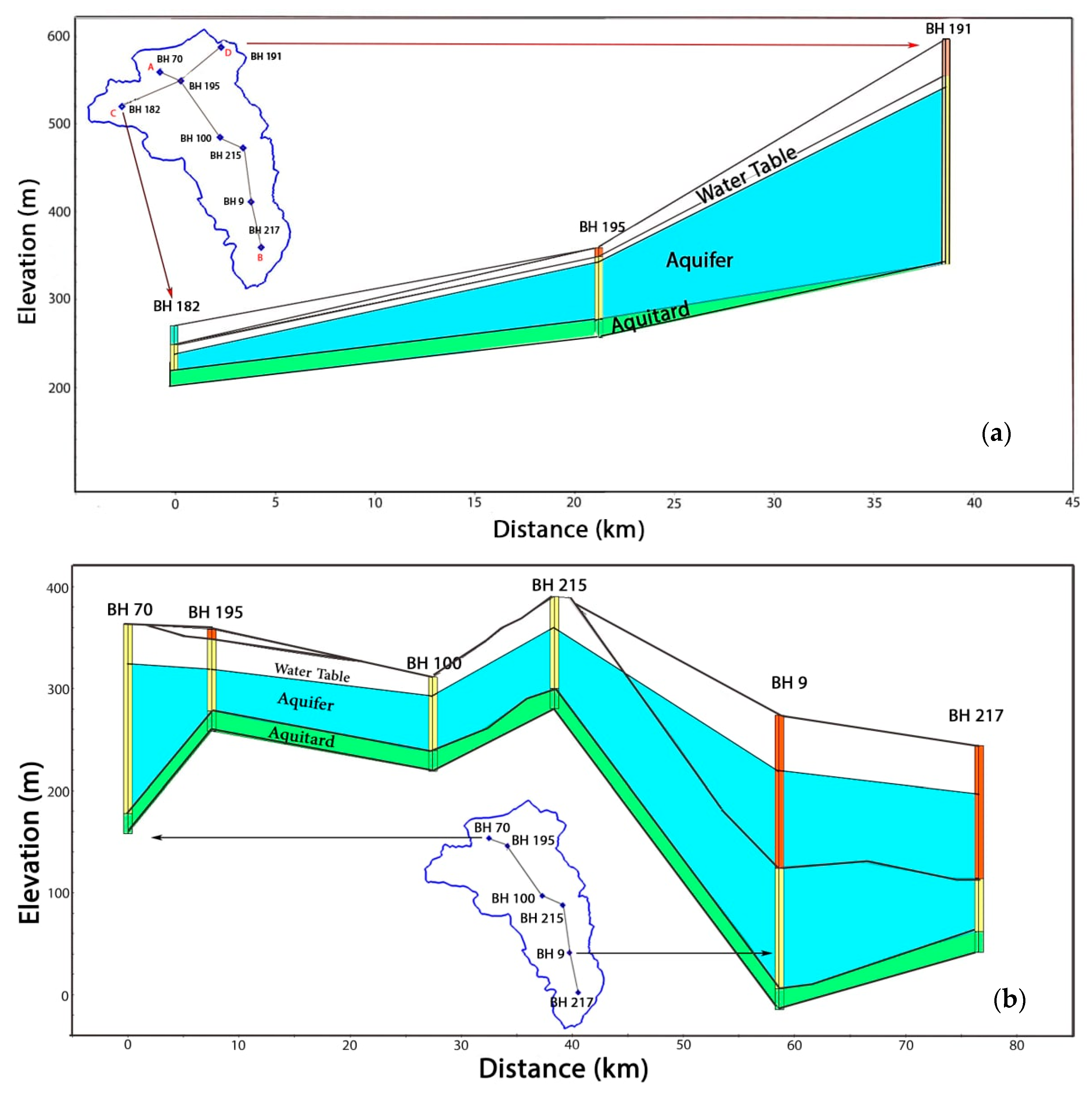
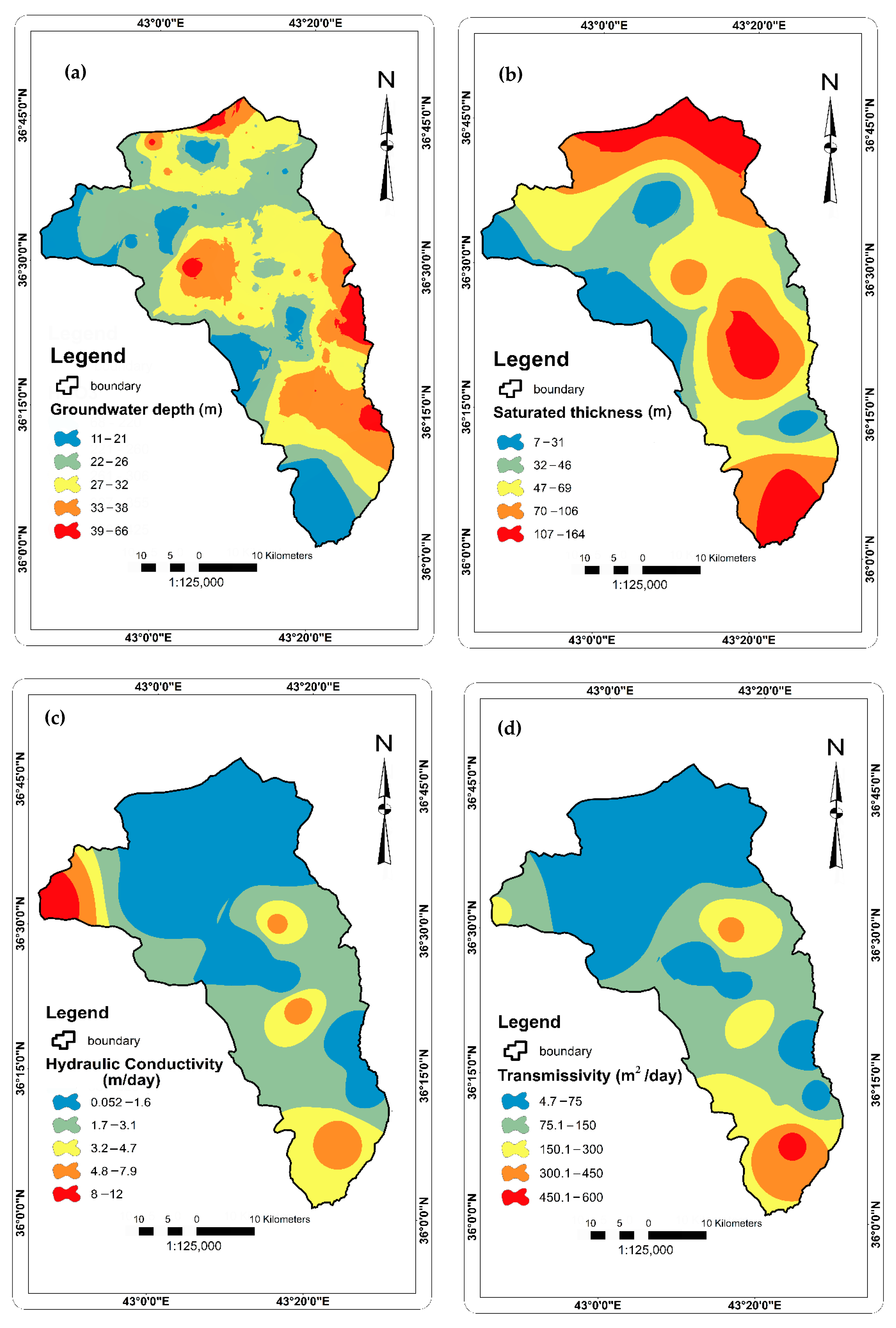
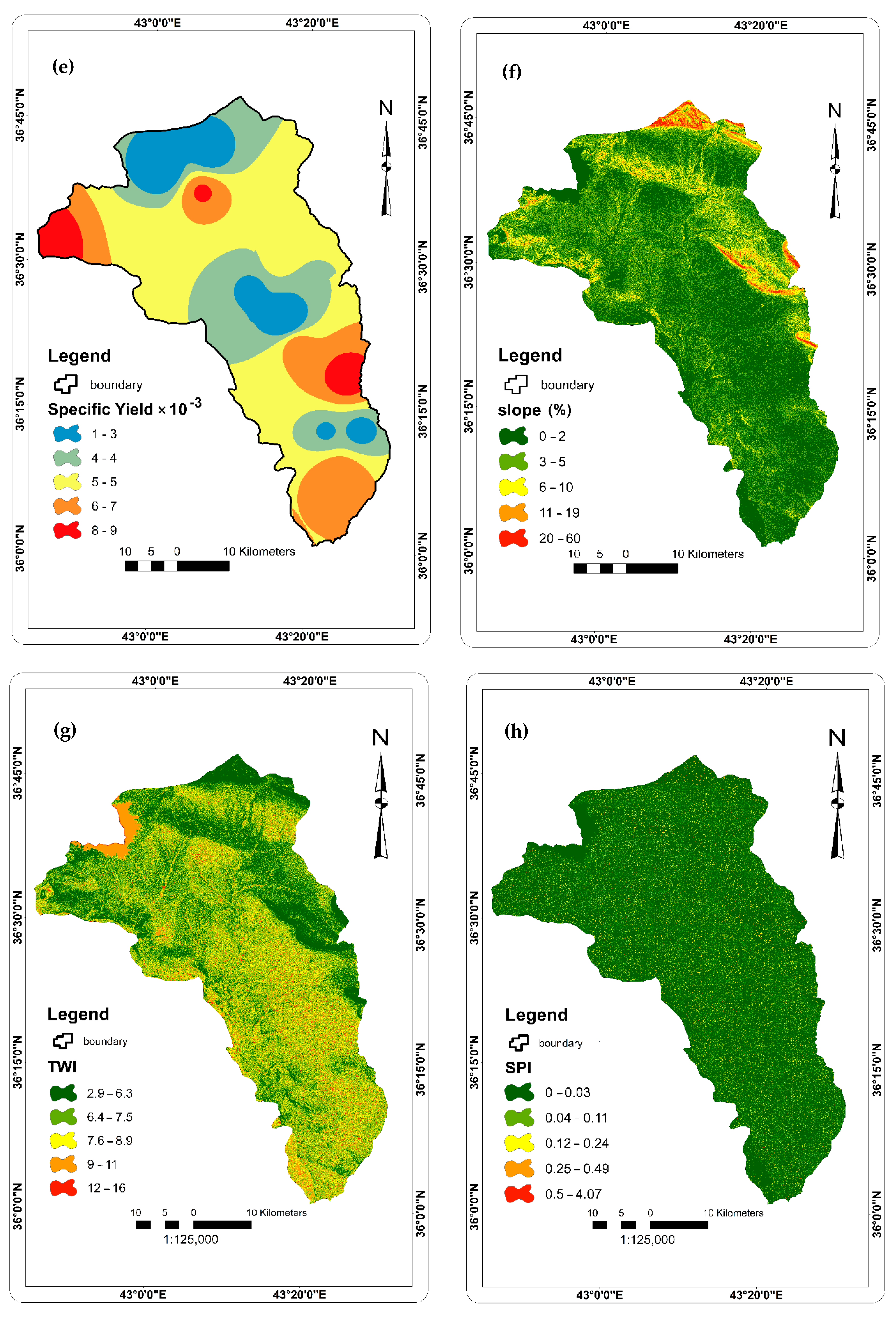
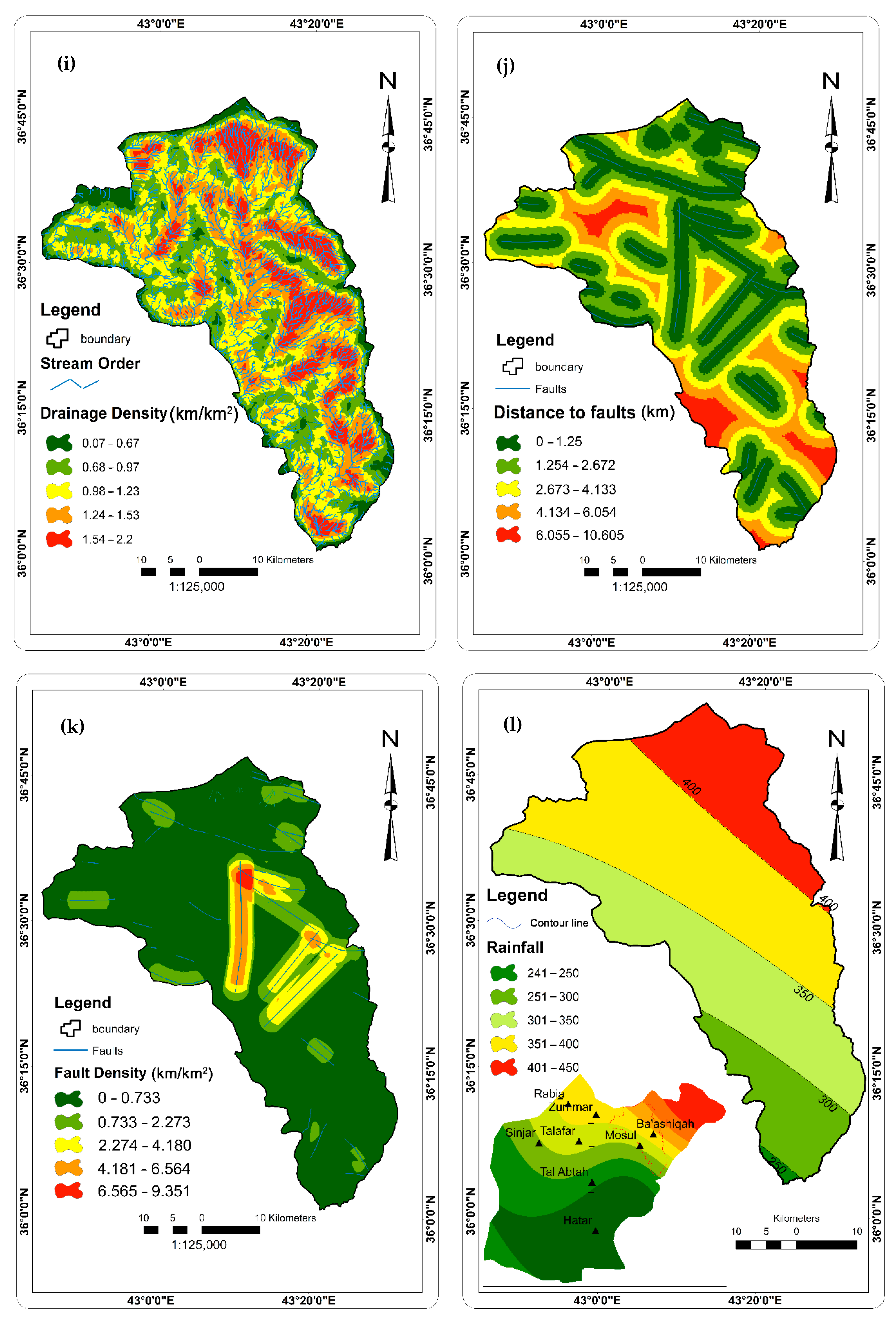
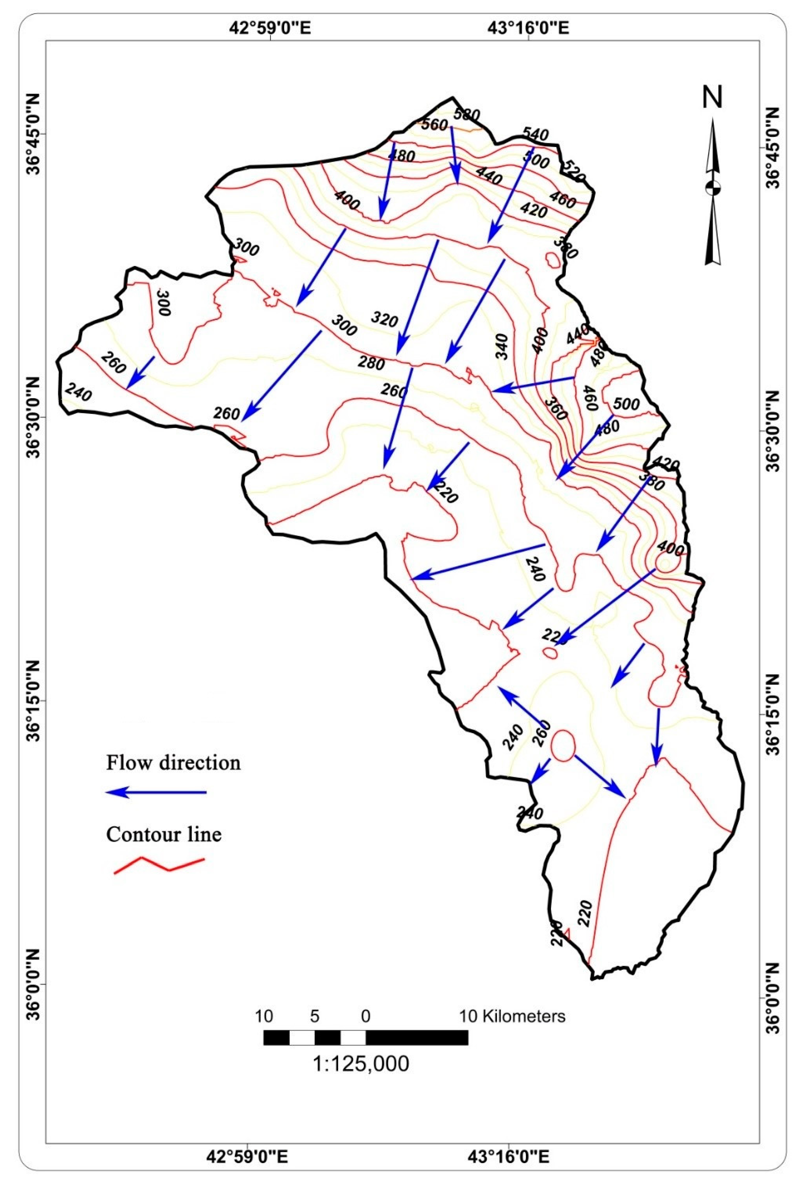
2.2.2. Factors Affecting Groundwater Occurrence and Availability
2.3. Feature Selection
2.4. Azure Cloud Platform and Machine Learning Classifiers Used
2.5. Error Statistics Used to Evaluate the Model Performances
3. Results
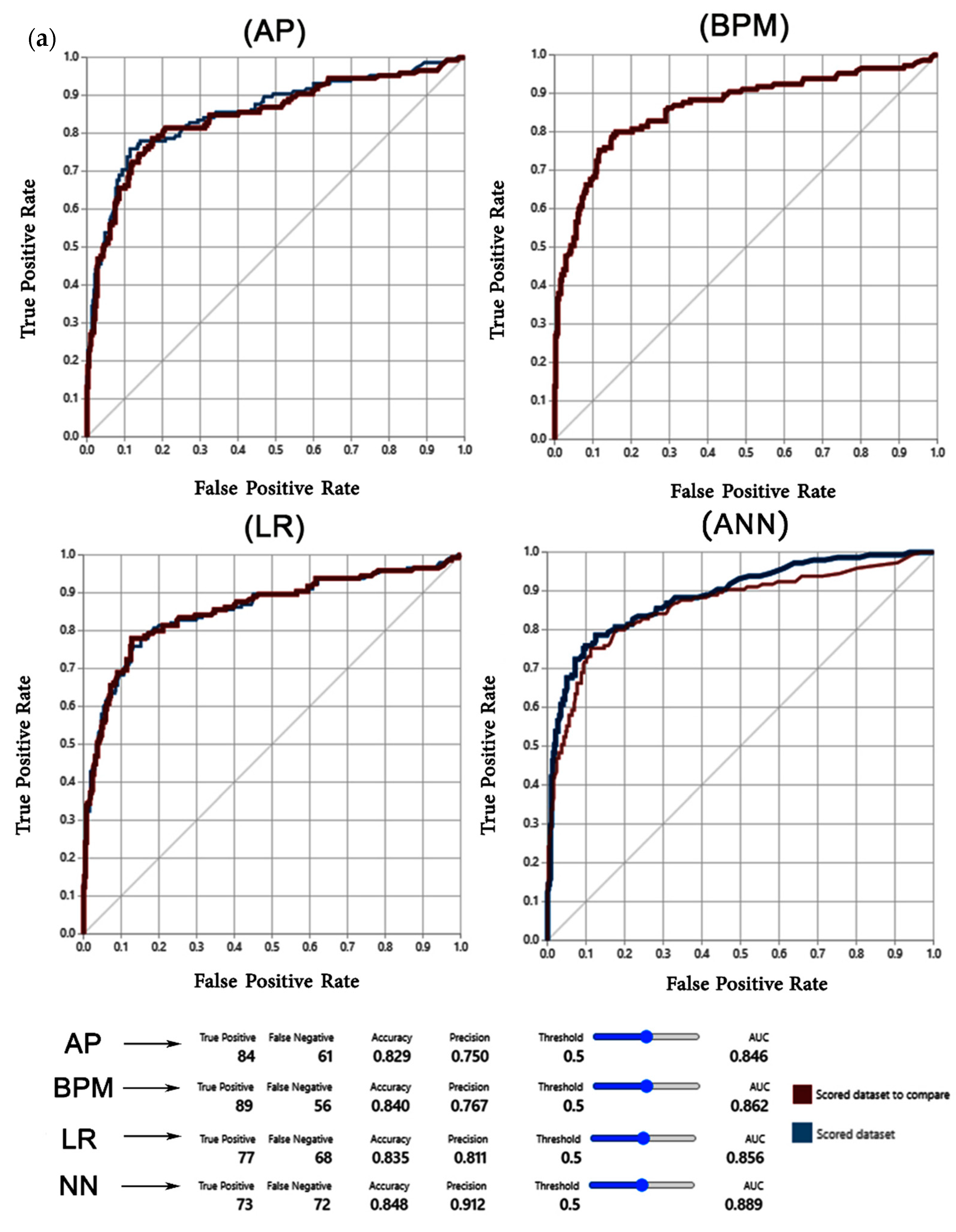
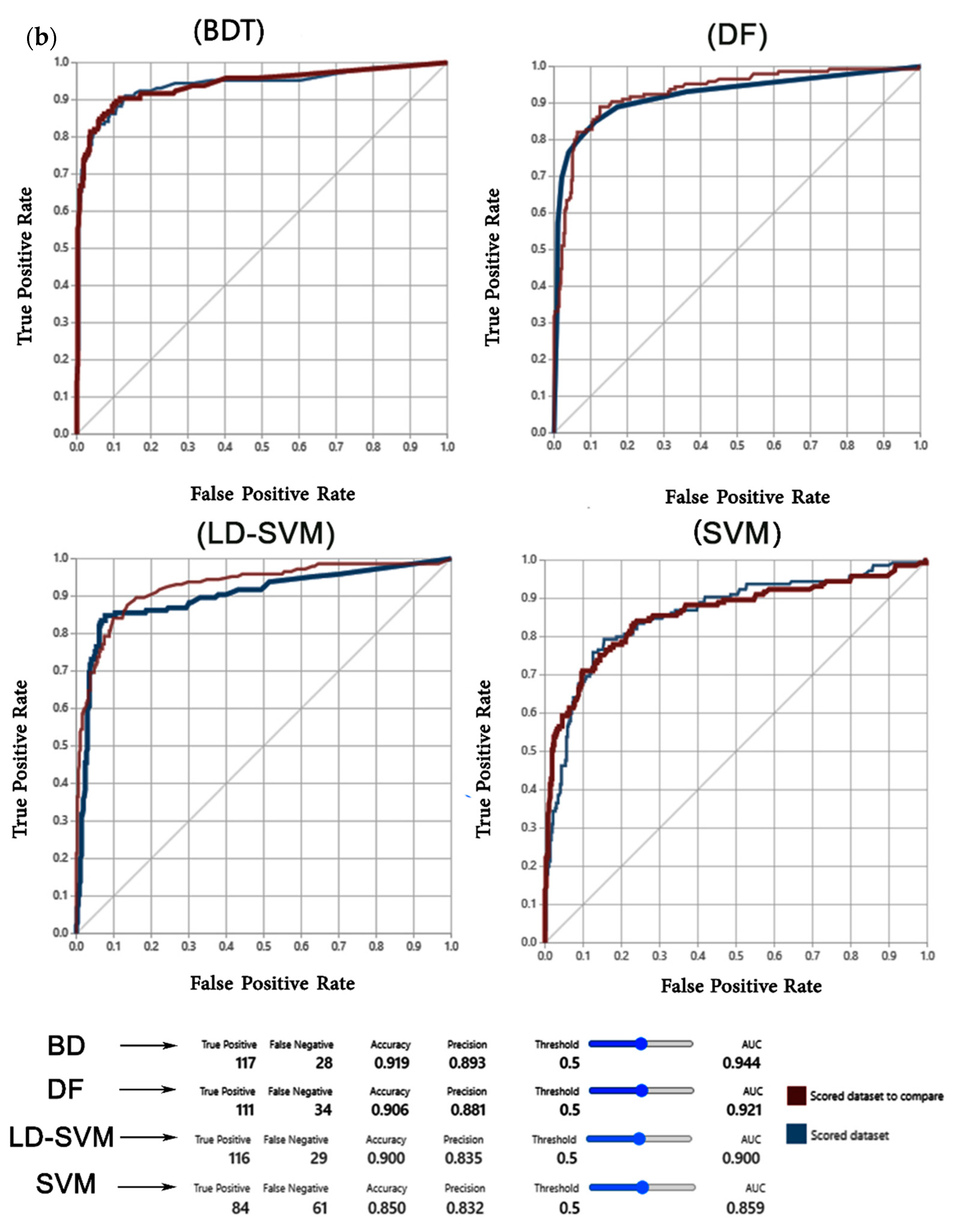
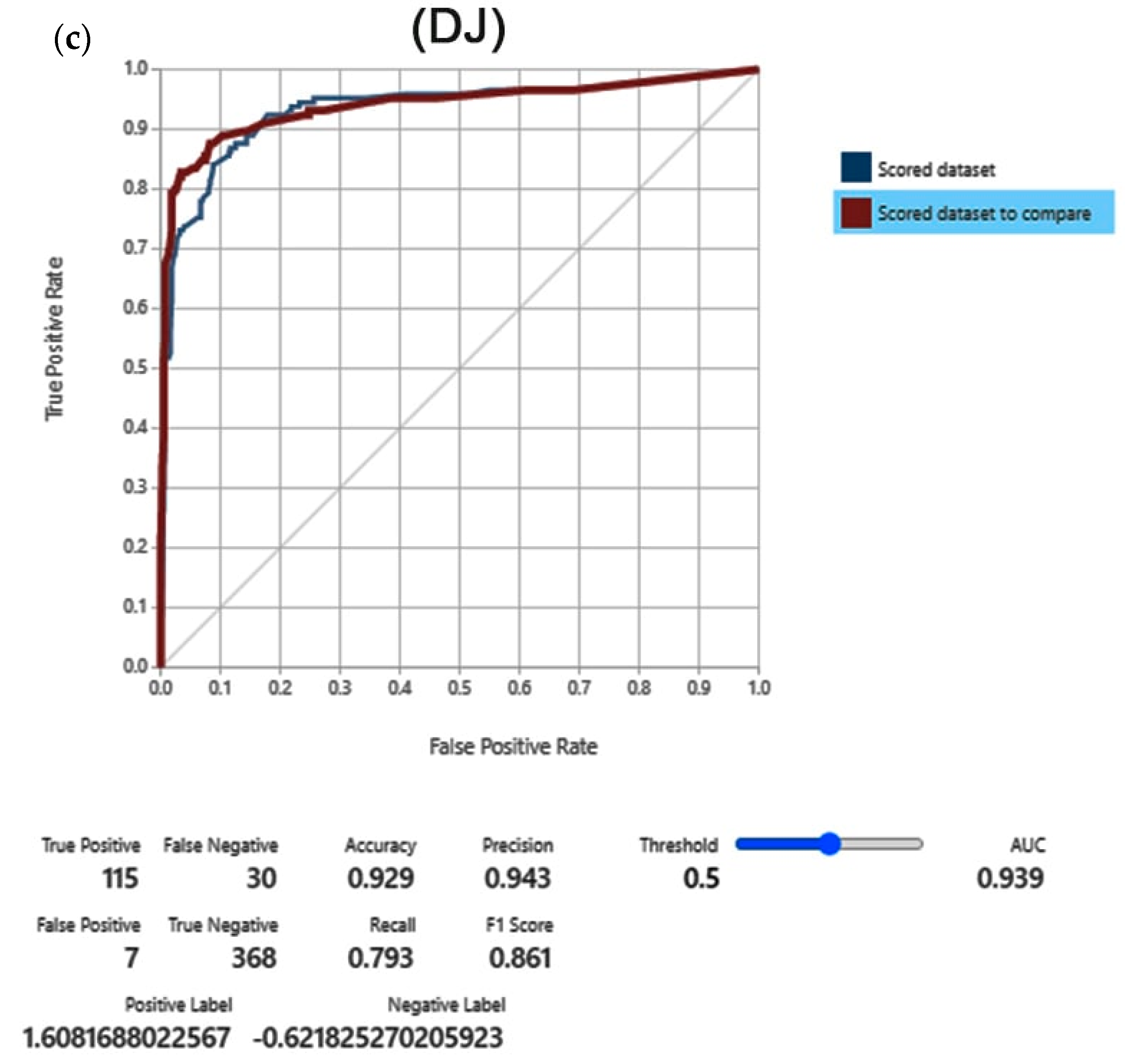
3.1. Results Validation
3.2. Source of Result Uncertainty
4. Discussion
4.1. Contribution of Groundwater Factors in Developing Groundwater Potential Map
4.2. Validation of the Models
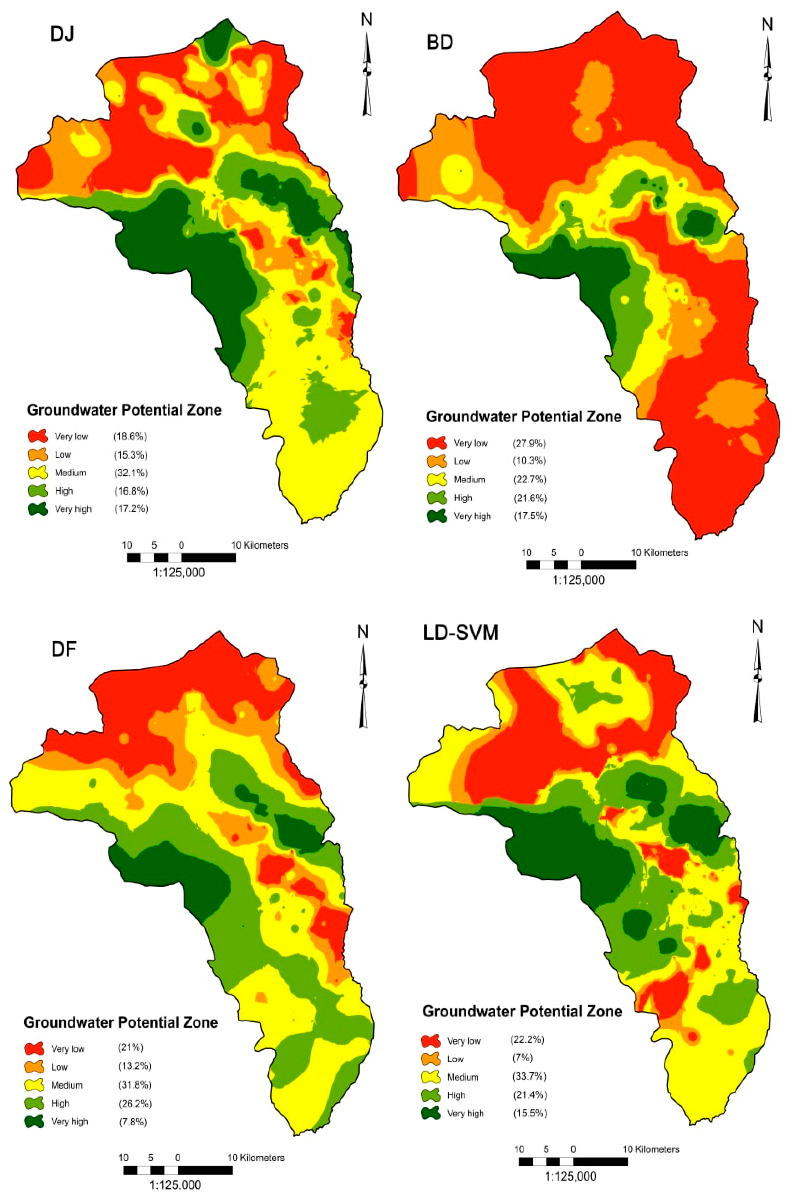
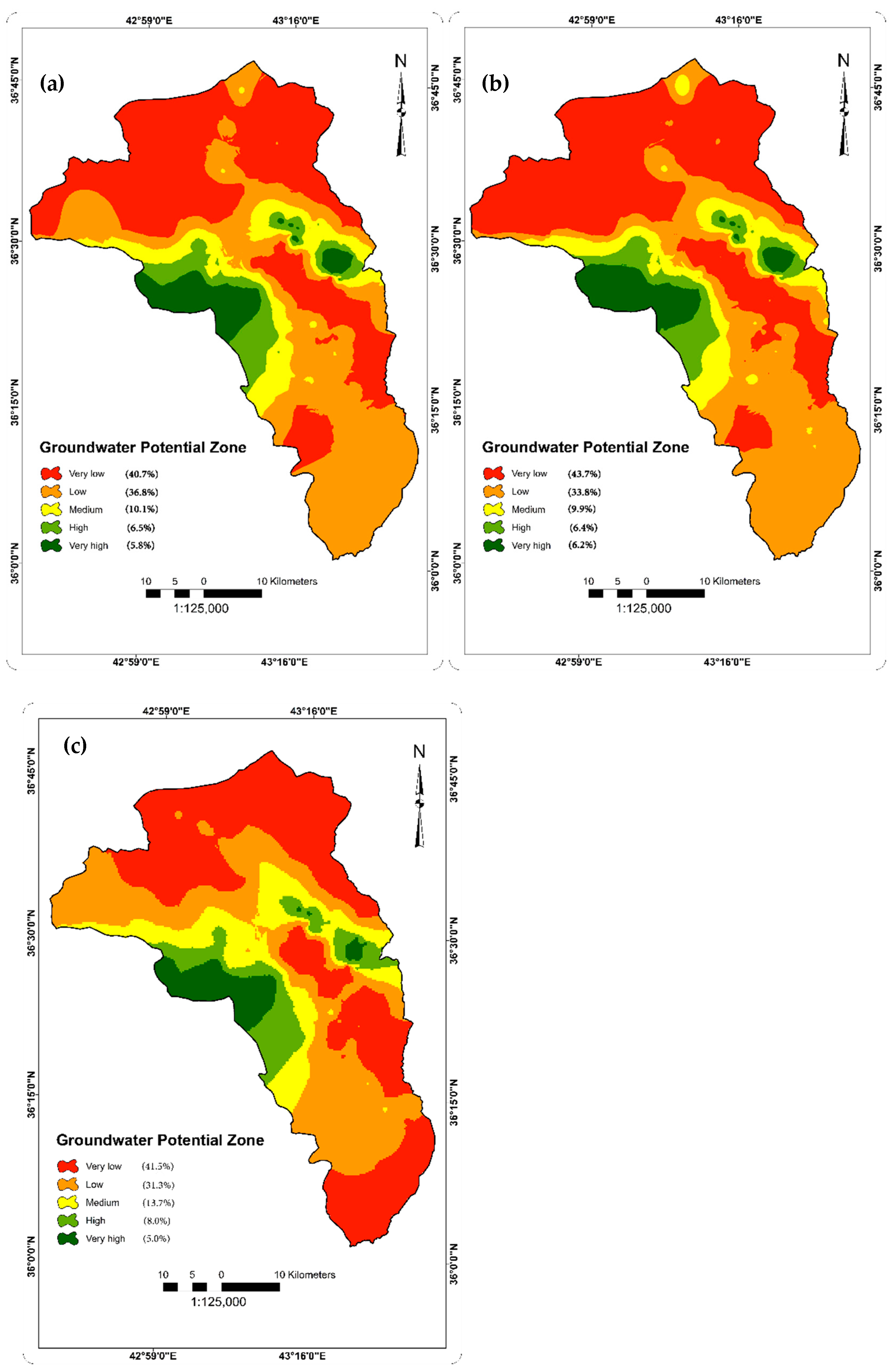
4.3. Distribution of Groundwater Potential Zones
5. Concluding Remarks
Author Contributions
Funding
Institutional Review Board Statement
Informed Consent Statement
Data Availability Statement
Acknowledgments
Conflicts of Interest
References
- Zektser, I.; Everett, L. Groundwater Resources of the World and Their Use, IHP-VI Ser; International Groundwater Resources Assessment Centre: Delft, The Netherlands, 2004; Volume 6, 346p. [Google Scholar]
- Famiglietti, J.S.; Lo, M.; Ho, S.L.; Bethune, J.; Anderson, K.; Syed, T.H.; Swenson, S.C.; de Linage, C.R.; Rodell, M. Satellites measure recent rates of groundwater depletion in California’s Central Valley. Geophys. Res. Lett. 2011, 38, 1–4. [Google Scholar] [CrossRef] [Green Version]
- Winter, T.C.; Harvey, J.W.; Franke, O.L.; Alley, W.M. Ground Water and Surface Water. A Single Resource. USGS Circular; Diane Publishing: Collingdale, PA, USA, 1999; Volume 1139. [Google Scholar]
- Díaz-Alcaide, S.; Martínez-Santos, P. Advances in groundwater potential mapping. Hydrogeol. J. 2019, 27, 2307–2324. [Google Scholar] [CrossRef]
- Al-Abadi, A.M.; Handhal, A.M.; Al-Ginamy, M.A. Evaluating the Dibdibba Aquifer Productivity at the Karbala–Najaf Plateau (Central Iraq) Using GIS-Based Tree Machine Learning Algorithms. Nat. Resour. Res. 2020, 29, 1989–2009. [Google Scholar] [CrossRef]
- Naghibi, S.A.; Moghaddam, D.D.; Kalantar, B.; Pradhan, B.; Kisi, O. A comparative assessment of GIS-based data mining models and a novel ensemble model in groundwater well potential mapping. J. Hydrol. 2017, 548, 471–483. [Google Scholar] [CrossRef]
- Rahmati, O.; Naghibi, S.A.; Shahabi, H.; Bui, D.T.; Pradhan, B.; Azareh, A.; Rafiei-Sardooi, E.; Samani, A.N.; Melesse, A.M. Groundwater spring potential modelling: Comprising the capability and robustness of three different modeling approaches. J. Hydrol. 2018, 565, 248–261. [Google Scholar] [CrossRef]
- Jha, M.K.; Chowdary, V.M.; Chowdhury, A. Groundwater assessment in Salboni Block, West Bengal (India) using remote sensing, geographical information system and multi-criteria decision analysis techniques. J. Hydrol. 2010, 18, 1713–1728. [Google Scholar] [CrossRef]
- Çelik, R. Evaluation of groundwater potential by GIS-based multicriteria decision making as a spatial prediction tool: Case study in the Tigris River Batman-Hasankeyf Sub-Basin, Turkey. Water 2019, 11, 2630. [Google Scholar] [CrossRef] [Green Version]
- Das, N.; Mukhopadhyay, S. Application of multi-criteria decision making technique for the assessment of groundwater potential zones: A study on Birbhum district, West Bengal, India. Environ. Dev. Sustain. 2020, 22, 931–955. [Google Scholar] [CrossRef]
- Singh, L.K.; Jha, M.K.; Chowdary, V. Assessing the accuracy of GIS-based Multi-Criteria Decision Analysis approaches for mapping groundwater potential. Ecol. Indic. 2018, 91, 24–37. [Google Scholar] [CrossRef]
- Al-Abadi, A.M. Modeling of groundwater productivity in northeastern Wasit Governorate, Iraq using frequency ratio and Shannon’s entropy Models. Appl. Water Sci. 2017, 7, 699–716. [Google Scholar] [CrossRef] [Green Version]
- Al-Abadi, A.M.; Fryar, A.E.; Rasheed, A.A.; Pradhan, B. Assessment of groundwater potential in terms of the availability and quality of the resource: A case study from Iraq. Environ. Earth Sci. 2021, 80, 1–22. [Google Scholar] [CrossRef]
- Davoudi Moghaddam, D.; Rahmati, O.; Haghizadeh, A.; Kalantari, Z. A modeling comparison of groundwater potential mapping in a mountain bedrock aquifer: QUEST, GARP, and RF models. Water 2020, 12, 679. [Google Scholar] [CrossRef] [Green Version]
- Abd Manap, M.; Sulaiman, W.N.A.; Ramli, M.F.; Pradhan, B.; Surip, N. A knowledge-driven GIS modeling technique for groundwater potential mapping at the Upper Langat Basin, Malaysia. Arab. J. Geosci. 2013, 6, 1621–1637. [Google Scholar] [CrossRef]
- Arulbalaji, P.; Padmalal, D.; Sreelash, K. GIS and AHP techniques based delineation of groundwater potential zones: A case study from southern Western Ghats, India. Sci. Rep. 2019, 9, 1–17. [Google Scholar] [CrossRef]
- Kumar, T.; Gautam, A.K.; Kumar, T. Appraising the accuracy of GIS-based multi-criteria decision making technique for delineation of groundwater potential zones. Water Resour. Manag. 2014, 28, 4449–4466. [Google Scholar] [CrossRef]
- Rahmati, O.; Samani, A.N.; Mahdavi, M.; Pourghasemi, H.R.; Zeinivand, H. Groundwater potential mapping at Kurdistan region of Iran using analytic hierarchy process and GIS. Arab. J. Geosci. 2015, 8, 7059–7071. [Google Scholar] [CrossRef]
- Chen, W.; Pradhan, B.; Li, S.; Shahabi, H.; Rizeei, H.M.; Hou, E.; Wang, S. Novel hybrid integration approach of bagging-based fisher’s linear discriminant function for groundwater potential analysis. Nat. Resour. Res. 2019, 28, 1239–1258. [Google Scholar] [CrossRef] [Green Version]
- Das, S. Comparison among influencing factor, frequency ratio, and analytical hierarchy process techniques for groundwater potential zonation in Vaitarna basin, Maharashtra, India. Groundw. Sustain. Dev. 2019, 8, 617–629. [Google Scholar] [CrossRef]
- Miraki, S.; Zanganeh, S.H.; Chapi, K.; Singh, V.P.; Shirzadi, A.; Shahabi, H.; Pham, B.T. Mapping groundwater potential using a novel hybrid intelligence approach. Water Resour. Manag. 2019, 33, 281–302. [Google Scholar] [CrossRef]
- Nguyen, P.T.; Ha, D.H.; Avand, M.; Jaafari, A.; Nguyen, H.D.; Al-Ansari, N.; Van Phong, T.; Sharma, R.; Kumar, R.; Le, H.V. Soft computing ensemble models based on logistic regression for groundwater potential mapping. Appl. Sci. 2020, 10, 2469. [Google Scholar] [CrossRef] [Green Version]
- Rahmati, O.; Pourghasemi, H.R.; Melesse, A.M. Application of GIS-based data driven random forest and maximum entropy models for groundwater potential mapping: A case study at Mehran Region, Iran. Catena 2016, 137, 360–372. [Google Scholar] [CrossRef]
- Hayley, K. The present state and future application of cloud computing for numerical groundwater modeling. Groundwater 2017, 55, 678–682. [Google Scholar] [CrossRef]
- Armbrust, M.; Fox, A.; Griffith, R.; Joseph, A.D.; Katz, R.; Konwinski, A.; Lee, G.; Patterson, D.; Rabkin, A.; Stoica, I. A view of cloud computing. Commun. ACM 2010, 53, 50–58. [Google Scholar] [CrossRef] [Green Version]
- Ganeshkumar, M.; Ramesh, V. A Study on Digital India Programme Using Azure Cloud and Twitter Data. Int. J. Comput. Intell. Res. 2017, 13, 781–790. [Google Scholar]
- Hayley, K.; Schumacher, J.; MacMillan, G.; Boutin, L. Highly parameterized model calibration with cloud computing: An example of regional flow model calibration in northeast Alberta, Canada. Hydrogeol. J. 2014, 22, 729–737. [Google Scholar] [CrossRef]
- Hunt, R.J.; Luchette, J.; Schreuder, W.A.; Rumbaugh, J.O.; Doherty, J.; Tonkin, M.J.; Rumbaugh, D.B. Using a cloud to replenish parched groundwater modeling efforts. Groundwater 2010, 48, 360–365. [Google Scholar] [CrossRef]
- Wang, D.; Xu, H.; Shi, Y.; Ding, Z.; Deng, Z.; Liu, Z.; Xu, X.; Lu, Z.; Wang, G.; Cheng, Z. The groundwater potential assessment system based on cloud computing: A case study in islands region. Comput. Commun. 2021, 178, 83–97. [Google Scholar] [CrossRef]
- Jassim, S.Z.; Goff, J.C. Geology of Iraq; Dolin, Prague and Moravian Museum: Brno, Czech Republic, 2006. [Google Scholar]
- Driscoll, F.G. Groundwater and Wells; Johnson Screens; U.S. Geological Survey: Washington, DC, USA, 1986; 799p.
- Al-Abadi, A.M.; Al-Temmeme, A.A.; Al-Ghanimy, M.A. A GIS-based combining of frequency ratio and index of entropy approaches for mapping groundwater availability zones at Badra–Al Al-Gharbi–Teeb areas, Iraq. Sustain. Water Resour. Manag. 2016, 2, 265–283. [Google Scholar] [CrossRef] [Green Version]
- Wada, Y.; Van Beek, L.P.; Van Kempen, C.M.; Reckman, J.W.; Vasak, S.; Bierkens, M.F. Global depletion of groundwater resources. Geophys. Res. Lett. 2010, 37, 1–5. [Google Scholar] [CrossRef] [Green Version]
- Al-Abadi, A.M.; Shahid, S. A comparison between index of entropy and catastrophe theory methods for mapping groundwater potential in an arid region. Environ. Monit. Assess. 2015, 187, 1–21. [Google Scholar] [CrossRef] [PubMed] [Green Version]
- Oh, H.-J.; Kim, Y.-S.; Choi, J.-K.; Park, E.; Lee, S. GIS mapping of regional probabilistic groundwater potential in the area of Pohang City, Korea. J. Hydrol. 2011, 399, 158–172. [Google Scholar] [CrossRef]
- Ozdemir, A. Using a binary logistic regression method and GIS for evaluating and mapping the groundwater spring potential in the Sultan Mountains (Aksehir, Turkey). J. Hydrol. 2011, 405, 123–136. [Google Scholar] [CrossRef]
- Beven, K.J.; Kirkby, M.J. A physically based, variable contributing area model of basin hydrology/Un modèle à base physique de zone d’appel variable de l’hydrologie du bassin versant. Hydrol. Sci. J. 1979, 24, 43–69. [Google Scholar] [CrossRef] [Green Version]
- Moore, I.D.; Grayson, R.; Ladson, A. Digital terrain modelling: A review of hydrological, geomorphological, and biological applications. Hydrol. Process. 1991, 5, 3–30. [Google Scholar] [CrossRef]
- Naghibi, S.A.; Pourghasemi, H.R.; Pourtaghi, Z.S.; Rezaei, A. Groundwater qanat potential mapping using frequency ratio and Shannon’s entropy models in the Moghan watershed, Iran. Earth Sci. Inform. 2015, 8, 171–186. [Google Scholar] [CrossRef]
- Alozeer, A.; Abdaki, M.A.; Al-Iraqi, A.; Al-Samman, S.; Al-Hammadi, N. Estimation of mean areal rainfall and missing data by using gis in nineveh, Northern Iraq. IGJ 2020, 93–103. [Google Scholar] [CrossRef]
- Subasi, A. Practical Machine Learning for Data Analysis Using Python; Academic Press: Cambridge, MA, USA, 2020. [Google Scholar]
- Brownlee, J. Master Machine Learning Algorithms: Discover how They Work and Implement Them from Scratch; Machine Learning Mastery: Boston, MA, USA, 2016. [Google Scholar]
- Bui, D.T.; Tuan, T.A.; Klempe, H.; Pradhan, B.; Revhaug, I. Spatial prediction models for shallow landslide hazards: A comparative assessment of the efficacy of support vector machines, artificial neural networks, kernel logistic regression, and logistic model tree. Landslides 2016, 13, 361–378. [Google Scholar]
- Wells, J.C.; Hung, T.T. Longman pronunciation dictionary. RELC J. 1990, 21, 95–97. [Google Scholar] [CrossRef]
- Hassoun, M.H. Fundamentals of Artificial Neural Networks; MIT Press: Cambridge, MA, USA, 1995. [Google Scholar]
- Yegnanarayana, B. Artificial Neural Networks; PHI Learning Pvt. Ltd.: New Delhi, India, 2009. [Google Scholar]
- Priddy, K.L.; Keller, P.E. Artificial Neural Networks: An Introduction; SPIE Press: Bellingham, WA, USA, 2005. [Google Scholar]
- Shanmuganathan, S. Artificial neural network modelling: An introduction. In Artificial Neural Network Modelling; Springer: Berlin/Heidelberg, Germany, 2016; pp. 1–14. [Google Scholar]
- Suthaharan, S. Machine learning models and algorithms for big data classification. Integr. Ser. Inf. Syst 2016, 36, 1–12. [Google Scholar]
- Cortes, C.; Vapnik, V. Support-vector networks. Mach. Learn. 1995, 20, 273–297. [Google Scholar] [CrossRef]
- Herbrich, R.; Graepel, T.; Campbell, C. Bayes point machines. J. Mach. Learn. Res. 2001, 1, 245–279. [Google Scholar]
- Shotton, J.; Sharp, T.; Kohli, P.; Nowozin, S.; Winn, J.; Criminisi, A. Decision jungles: Compact and rich models for classification. In Proceedings of the NIPS’13 Proceedings of the 26th International Conference on Neural Information Processing Systems, Lake Tahoe, NV, USA, 5–10 December 2013; pp. 234–242. [Google Scholar]
- Ghasemkhani, N.; Vayghan, S.S.; Abdollahi, A.; Pradhan, B.; Alamri, A. Urban Development Modeling Using Integrated Fuzzy Systems, Ordered Weighted Averaging (OWA), and Geospatial Techniques. Sustainability 2020, 12, 809. [Google Scholar] [CrossRef] [Green Version]
- Arabameri, A.; Rezaei, K.; Cerda, A.; Lombardo, L.; Rodrigo-Comino, J. GIS-based groundwater potential mapping in Shahroud plain, Iran. A comparison among statistical (bivariate and multivariate), data mining and MCDM approaches. Sci. Total Environ. 2019, 658, 160–177. [Google Scholar] [CrossRef] [PubMed]
- Razavi-Termeh, S.V.; Sadeghi-Niaraki, A.; Choi, S.-M. Groundwater potential mapping using an integrated ensemble of three bivariate statistical models with random forest and logistic model tree models. Water 2019, 11, 1596. [Google Scholar] [CrossRef] [Green Version]
- Chen, W.; Zhao, X.; Tsangaratos, P.; Shahabi, H.; Ilia, I.; Xue, W.; Wang, X.; Ahmad, B.B. Evaluating the usage of tree-based ensemble methods in groundwater spring potential mapping. J. Hydrol. 2020, 583, 124602. [Google Scholar] [CrossRef]
- Naghibi, S.A.; Pourghasemi, H.R.; Dixon, B. GIS-based groundwater potential mapping using boosted regression tree, classification and regression tree, and random forest machine learning models in Iran. Environ. Monit. Assess. 2016, 188, 1–27. [Google Scholar] [CrossRef] [PubMed]
- Lee, S.; Hyun, Y.; Lee, S.; Lee, M.-J. Groundwater potential mapping using remote sensing and GIS-based machine learning techniques. Remote Sens. 2020, 12, 1200. [Google Scholar] [CrossRef] [Green Version]
- Prasad, P.; Loveson, V.J.; Kotha, M.; Yadav, R. Application of machine learning techniques in groundwater potential mapping along the west coast of India. GIScience Remote Sens. 2020, 57, 735–752. [Google Scholar] [CrossRef]
- Kordestani, M.D.; Naghibi, S.A.; Hashemi, H.; Ahmadi, K.; Kalantar, B.; Pradhan, B. Groundwater potential mapping using a novel data-mining ensemble model. Hydrogeol. J. 2019, 27, 211–224. [Google Scholar] [CrossRef] [Green Version]
- Kamali Maskooni, E.; Naghibi, S.A.; Hashemi, H.; Berndtsson, R. Application of advanced machine learning algorithms to assess groundwater potential using remote sensing-derived data. Remote Sens. 2020, 12, 2742. [Google Scholar] [CrossRef]
- Sachdeva, S.; Kumar, B. Comparison of gradient boosted decision trees and random forest for groundwater potential mapping in Dholpur (Rajasthan), India. Stoch. Environ. Res. Risk Assess. 2021, 35, 287–306. [Google Scholar] [CrossRef]


| Formation | Age | Environment | Description |
|---|---|---|---|
| Pila spi | Middle–Upper Eocene | Shallow marine | Limestone and dolomite limestone |
| Fatha | Middle Miocene | Shallow marine | Anhydrite, mudstone, and thin limestone |
| Injana | Upper Miocene | Sub-marine | Red or gray colored silty marl or clay stones and purple silt stones |
| Muqdadyia | Pliocene | Continental | Gravely sandstone, sandstone, and red mudstone |
| Bai Hassan | Late Pliocene | Continental | Conglomerate with sandstone, silt stone, and claystone |
| Quaternary | Pleistocene–Holocene | Continental | Mixture of gravel, sand, silt, and clay |
| Attribute | Average Merit | Average Rank |
|---|---|---|
| Aquifer saturated thickness | 0.310 ± 0.016 | 1.0 ± 0.00 |
| Rainfall | 0.238 ± 0.038 | 2.7 ± 1.42 |
| Hydraulic conductivity | 0.189 ± 0.013 | 3.3 ± 1.19 |
| Depth to groundwater | 0.185 ± 0.008 | 4.0 ± 0.63 |
| Specific yield | 0.183 ± 0.015 | 4.2 ± 0.75 |
| Elevation | 0.161 ± 0.007 | 5.8 ± 0.40 |
| Geology | 0.062 ± 0.004 | 7.3 ± 0.44 |
| Fault density | 0.058 ± 0.013 | 8.2 ± 0.98 |
| Drainage density | 0.048 ± 0.004 | 9.6 ± 1.02 |
| Soil | 0.048 ± 0.003 | 9.7 ± 1.10 |
| LULC | 0.046 ± 0.007 | 10.6 ± 1.02 |
| Distance to faults | 0.038 ± 0.005 | 11.6 ± 0.92 |
| TWI | 0.000 ± 0.000 | 13.1 ± 0.30 |
| Slope | 0.000 ± 0.000 | 13.9 ± 0.30 |
| SPI | 0.000 ± 0.000 | 15.0 ± 0.00 |
| Model | Error Measures Used | |||||||||
|---|---|---|---|---|---|---|---|---|---|---|
| Training Phase | Testing Phase | |||||||||
| ACC | AUC | Precision | Recall | F-Score | ACC | AUC | Precision | Recall | F-Score | |
| AP | 0.84 | 0.86 | 0.76 | 0.59 | 0.66 | 0.83 | 0.85 | 0.75 | 0.58 | 0.65 |
| LR | 0.85 | 0.87 | 0.82 | 0.54 | 0.65 | 0.84 | 0.86 | 0.81 | 0.53 | 0.64 |
| BPM | 0.85 | 0.87 | 0.78 | 0.62 | 0.69 | 0.84 | 0.86 | 0.77 | 0.61 | 0.68 |
| NN | 0.86 | 0.90 | 0.92 | 0.51 | 0.66 | 0.85 | 0.89 | 0.91 | 0.50 | 0.65 |
| SVM | 0.86 | 0.87 | 0.84 | 0.59 | 0.69 | 0.85 | 0.86 | 0.83 | 0.58 | 0.68 |
| LD-SVM | 0.91 | 0.91 | 0.85 | 0.81 | 0.83 | 0.90 | 0.90 | 0.84 | 0.80 | 0.82 |
| DF | 0.92 | 0.93 | 0.89 | 0.78 | 0.83 | 0.91 | 0.92 | 0.88 | 0.77 | 0.82 |
| BDT | 0.93 | 0.95 | 0.90 | 0.82 | 0.86 | 0.92 | 0.94 | 0.89 | 0.81 | 0.85 |
| DJ | 0.94 | 0.95 | 0.95 | 0.80 | 0.87 | 0.93 | 0.94 | 0.94 | 0.79 | 0.86 |
| Groundwater Potential Zone | Algorithms Used | |||||||
|---|---|---|---|---|---|---|---|---|
| DJ | BDT | DF | LD-SVM | |||||
| Area (%) | Area (km2) | Area (%) | Area (km2) | Area (%) | Area (km2) | Area (%) | Area (km2) | |
| Very low–low | 33.9 | 862 | 38 | 973 | 34.2 | 870 | 29.3 | 744 |
| Moderate | 32.1 | 816 | 23 | 576 | 31.8 | 806 | 33.8 | 856 |
| High–very high | 34.0 | 862 | 39 | 991 | 34.0 | 864 | 36.9 | 940 |
Publisher’s Note: MDPI stays neutral with regard to jurisdictional claims in published maps and institutional affiliations. |
© 2021 by the authors. Licensee MDPI, Basel, Switzerland. This article is an open access article distributed under the terms and conditions of the Creative Commons Attribution (CC BY) license (https://creativecommons.org/licenses/by/4.0/).
Share and Cite
Al-Ozeer, A.Z.; Al-Abadi, A.M.; Hussain, T.A.; Fryar, A.E.; Pradhan, B.; Alamri, A.; Abdul Maulud, K.N. Modeling of Groundwater Potential Using Cloud Computing Platform: A Case Study from Nineveh Plain, Northern Iraq. Water 2021, 13, 3330. https://doi.org/10.3390/w13233330
Al-Ozeer AZ, Al-Abadi AM, Hussain TA, Fryar AE, Pradhan B, Alamri A, Abdul Maulud KN. Modeling of Groundwater Potential Using Cloud Computing Platform: A Case Study from Nineveh Plain, Northern Iraq. Water. 2021; 13(23):3330. https://doi.org/10.3390/w13233330
Chicago/Turabian StyleAl-Ozeer, Ali ZA., Alaa M. Al-Abadi, Tariq Abed Hussain, Alan E. Fryar, Biswajeet Pradhan, Abdullah Alamri, and Khairul Nizam Abdul Maulud. 2021. "Modeling of Groundwater Potential Using Cloud Computing Platform: A Case Study from Nineveh Plain, Northern Iraq" Water 13, no. 23: 3330. https://doi.org/10.3390/w13233330