
The Influence of Internal Erosion in Earthen Dams on the Potential Difference Response to Applied Voltage


Abstract
:1. Introduction
2. Materials and Methods
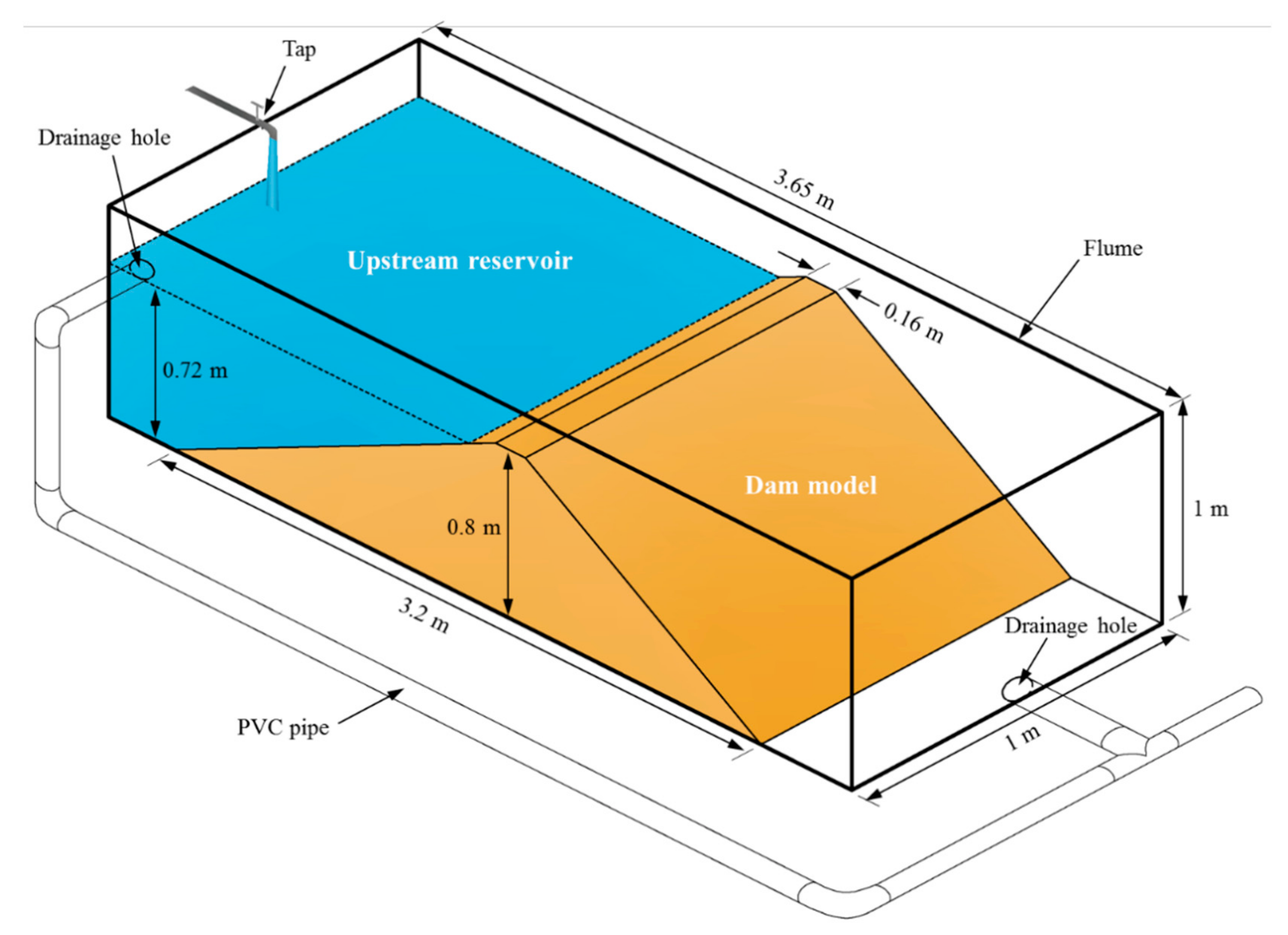
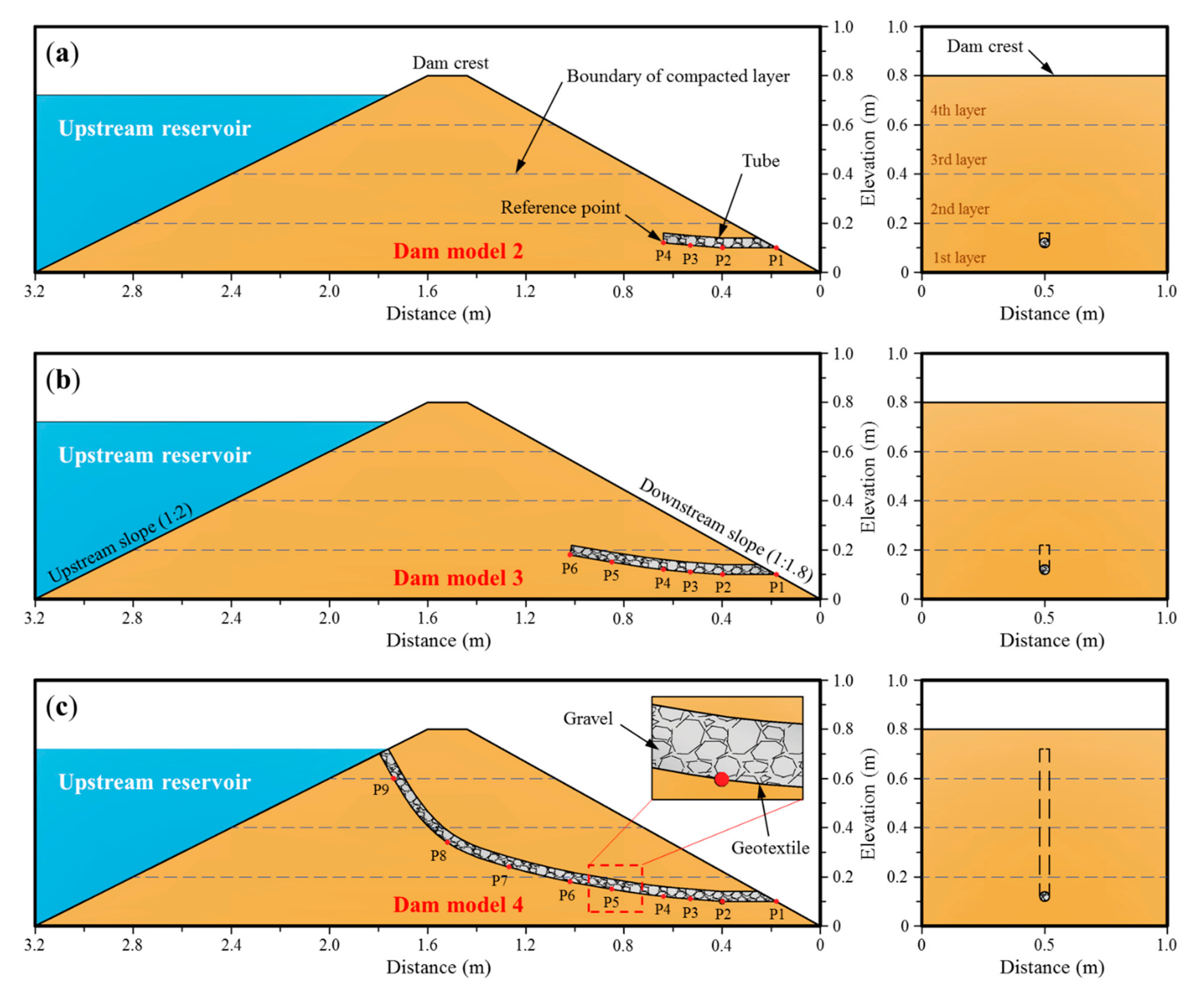
2.1. Experimental Setup
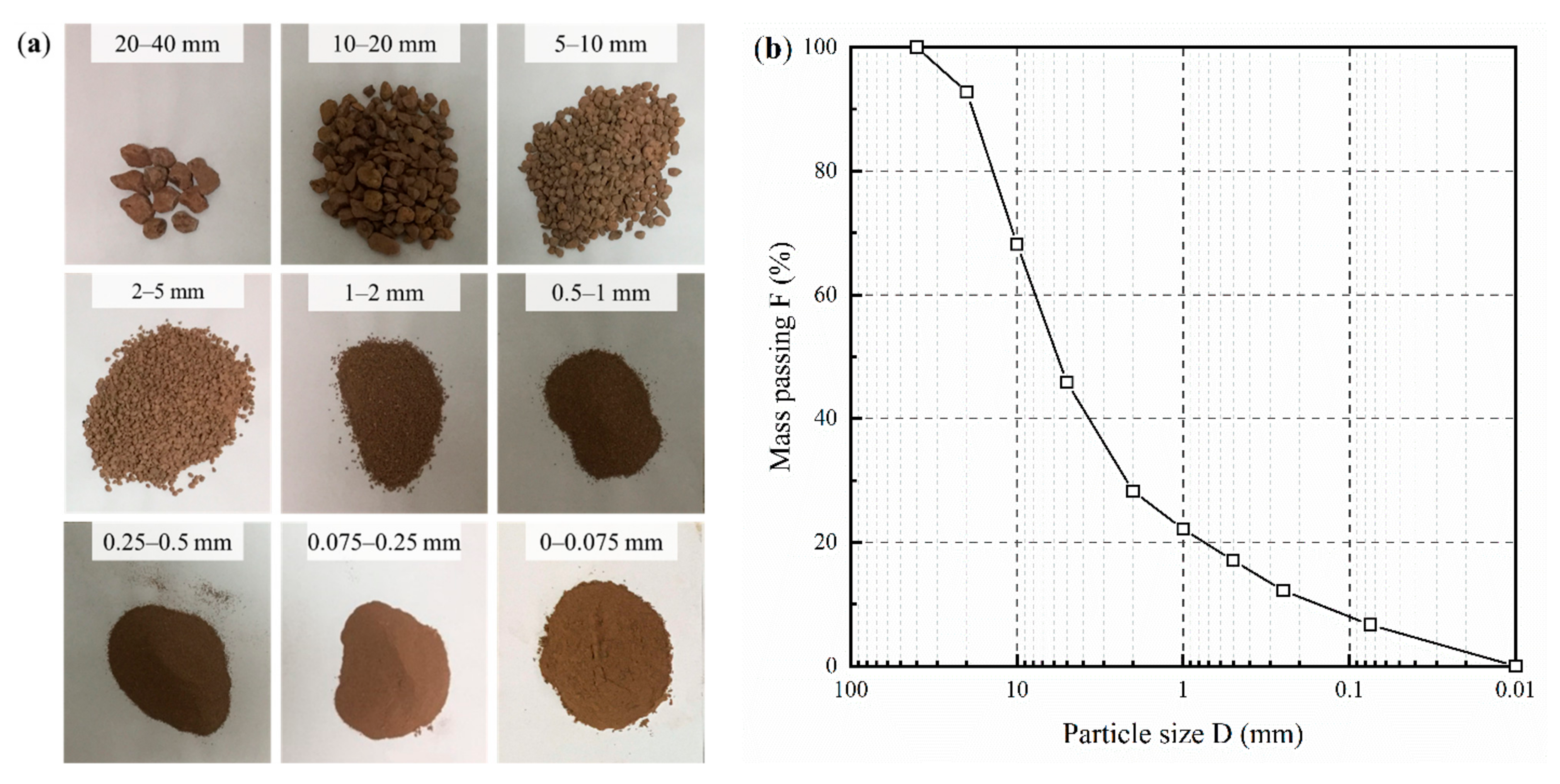
2.2. Soil Materials
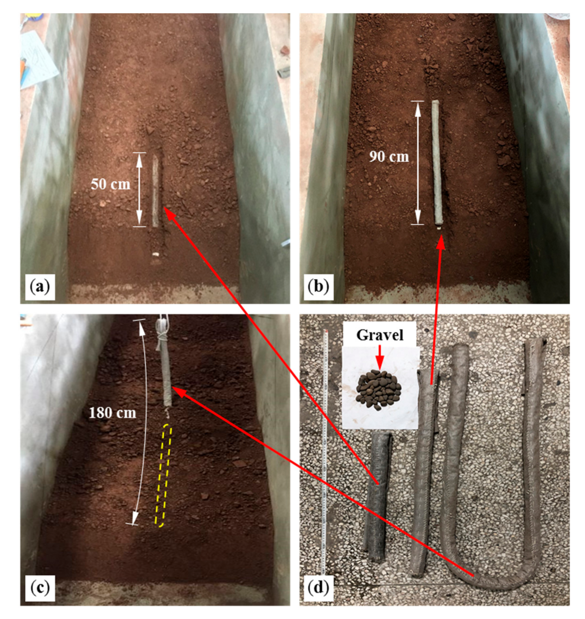
2.3. Test Procedure
3. Experimental Results
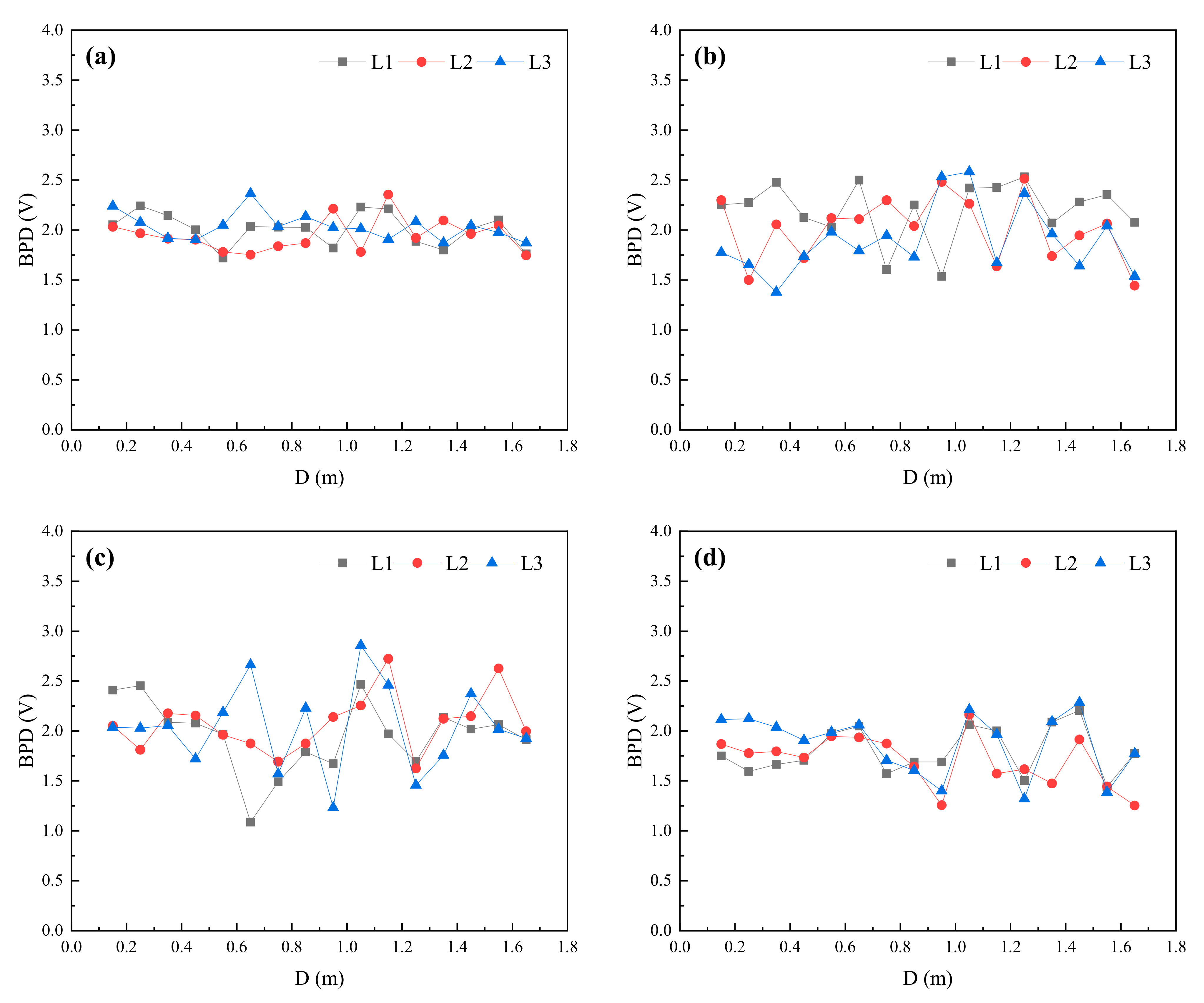
3.1. BPD of the Dam Models
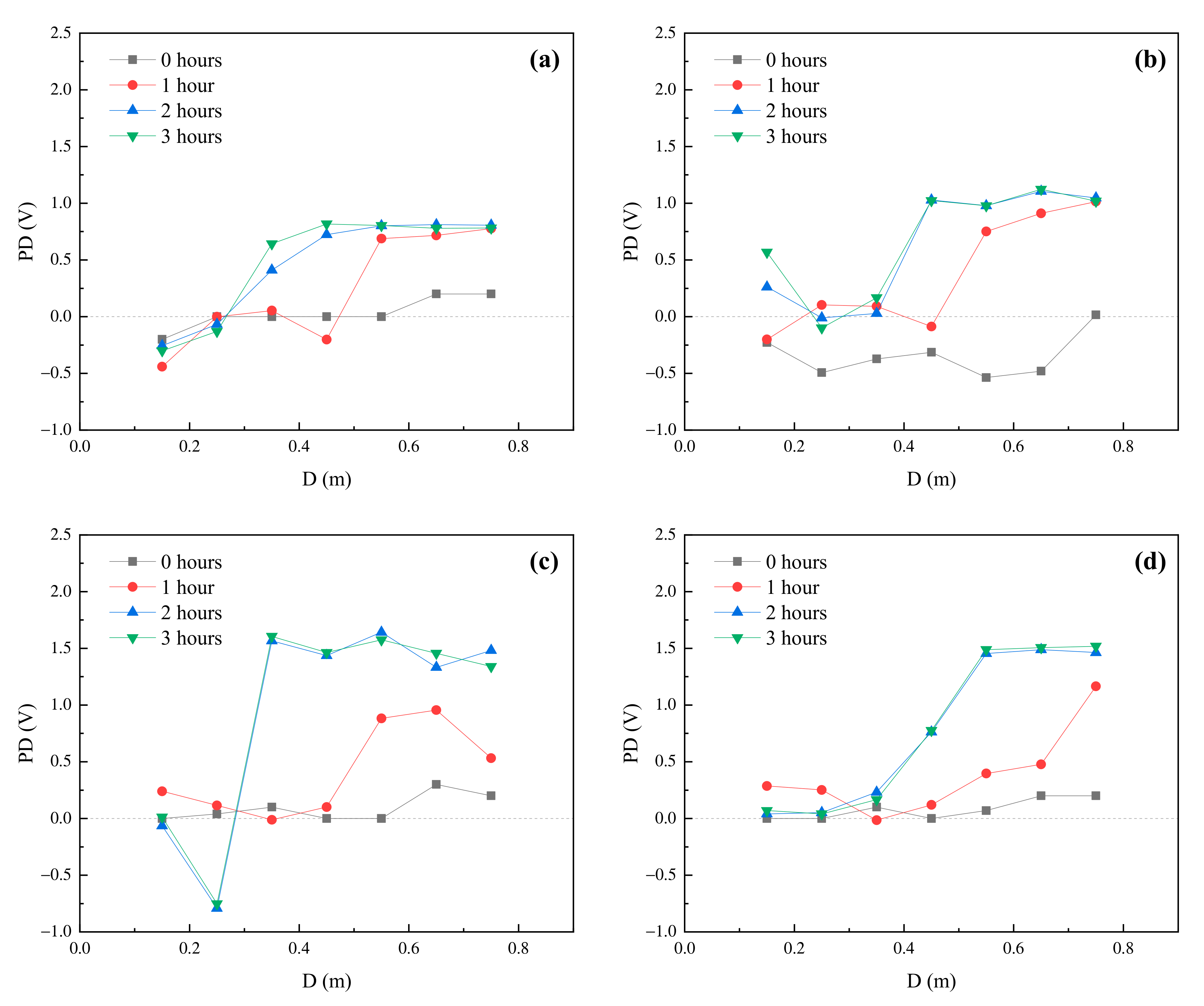
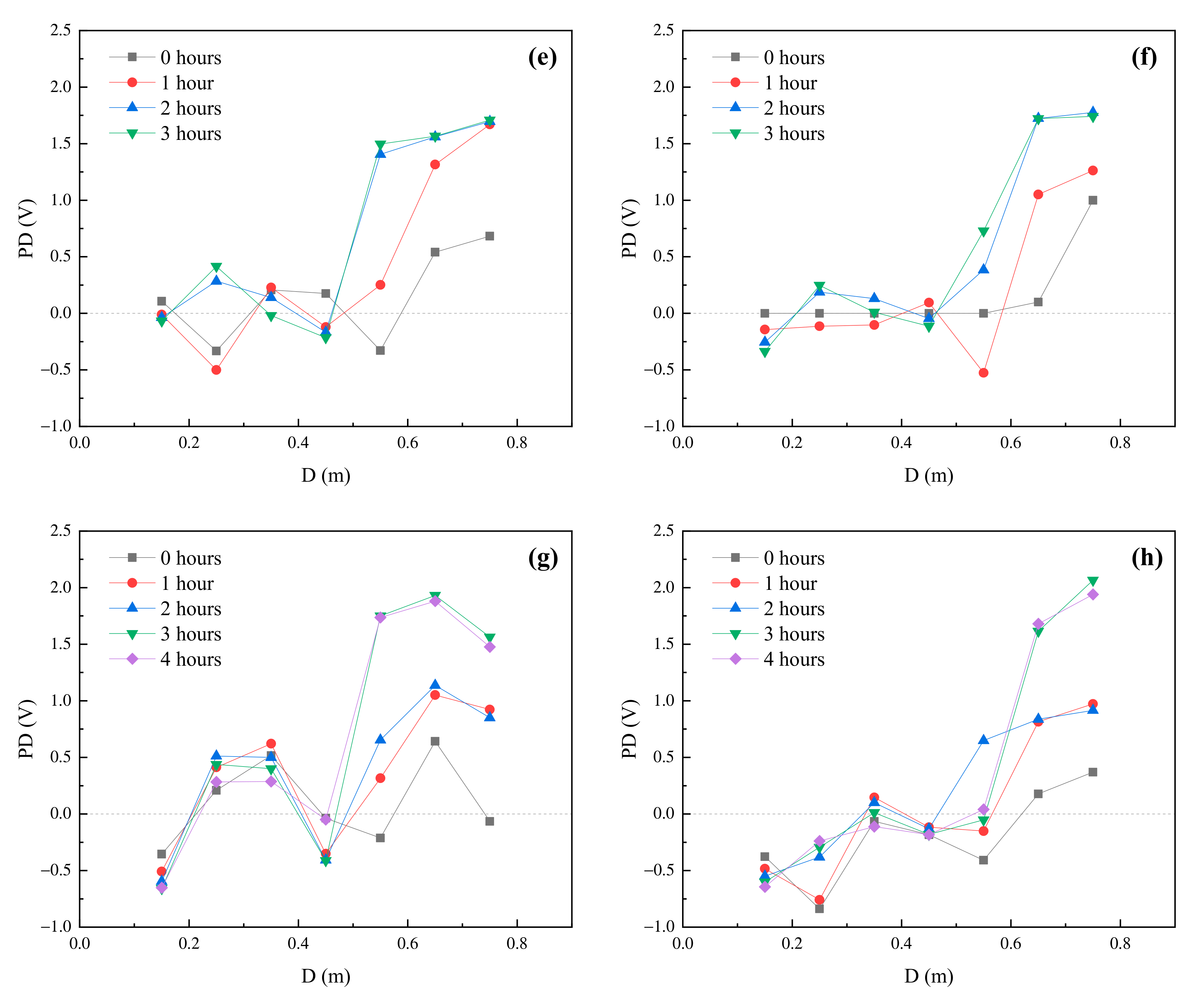
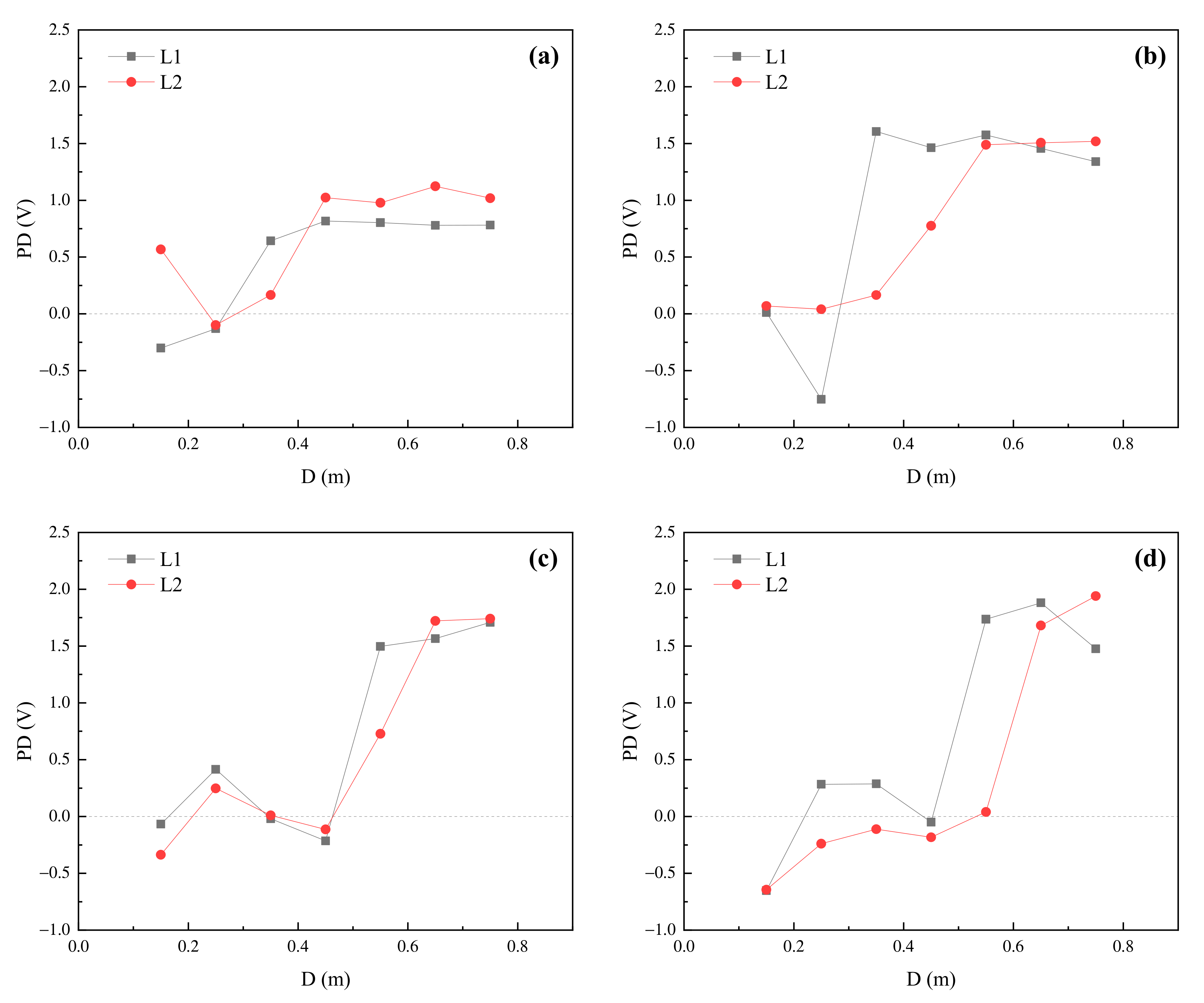
3.2. PD of the Dam Models under Seepage
4. Discussion
4.1. Discrepancy of Dam Models
4.2. Influence of Soil Moisture Content on PD
4.3. Influence of Internal Erosion on PD
5. Conclusions
- (1)
- Employing different dam models to simulate the development of internal erosion is acceptable. Due to the inevitable discrepancy among the models, extra attention should be paid to the background data of target measurement parameters, which determine the availability of the measurement results.
- (2)
- The moisture content of the soil has a significant effect on the PD response to applied voltage. The PD increases with an increase in soil moisture content until the soil is saturated, which is helpful to understand the change in the seepage state in earthen dams.
- (3)
- There is a remarkable correlation between the internal erosion and the PD response to applied voltage. Induced by the internal erosion, the starting position for the steep increase in PD moves toward the dam toe. This change is a continuing process as the erosion develops. The progression of internal erosion can be effectively traced through analyzing the PD. In the measured PD, the starting position for the steep increase is a reliable identification indicator, which lays a foundation for developing a PD-based approach to the monitoring and early warning of internal erosion in earthen dams.
- (4)
- It is noted that a measurement error can be induced by electrode stability. In addition, an error may be induced due to the mechanical properties of internal erosion, which is neglected in this study. These can provide a direction for further investigations.
Author Contributions
Funding
Institutional Review Board Statement
Informed Consent Statement
Data Availability Statement
Acknowledgments
Conflicts of Interest
References
- Altinbilek, D. The role of dams in development. Int. J. Water Resour. Dev. 2002, 18, 9–24. [Google Scholar] [CrossRef]
- Xu, J.B.; Wei, W.; Bao, H.; Zhang, K.K.; Lan, H.X.; Yan, C.G.; Sun, W.F. Failure models of a loess stacked dam: A case study in the Ansai Area (China). Bull. Eng. Geol. Environ. 2020, 79, 1009–1021. [Google Scholar] [CrossRef]
- Dhiman, S.; Patra, K.C. Studies of dam disaster in India and equations for breach parameter. Nat. Hazards 2019, 98, 783–807. [Google Scholar] [CrossRef]
- Saghaee, G.; Mousa, A.A.; Meguid, M.A. Plausible failure mechanisms of wildlife-damaged earth levees: Insights from centrifuge modeling and numerical analysis. Can. Geotech. J. 2017, 54, 1496–1508. [Google Scholar] [CrossRef] [Green Version]
- Benahmed, N.; Bonelli, S. Investigating concentrated leak erosion behaviour of cohesive soils by performing hole erosion tests. Eur. J. Environ. Civ. Eng. 2012, 16, 43–58. [Google Scholar] [CrossRef]
- Kojima, H.; Kohgo, Y.; Shimada, K.; Shoda, D.; Suzuki, H.; Saito, H. Numerical modeling of flood flow after small earthen dam failure: A case study from the 2011 Tohoku earthquake. Paddy Water Environ. 2020, 18, 431–442. [Google Scholar] [CrossRef]
- Andreini, M.; Gardoni, P.; Pagliara, S.; Sassu, M. Probabilistic models for erosion parameters and reliability analysis of earth dams and levees. ASCE-ASME J. Risk. Uncertain. Eng. Syst. Part A Civ. Eng. 2016, 2, 04016006. [Google Scholar] [CrossRef]
- Richards, K.S.; Reddy, K.R. Critical appraisal of piping phenomena in earth dams. Bull. Eng. Geol. Environ. 2007, 66, 381–402. [Google Scholar] [CrossRef]
- Foster, M.; Fell, R.; Spannagle, M. The statistics of embankment dam failures and accidents. Can. Geotech. J. 2000, 37, 1000–1024. [Google Scholar] [CrossRef]
- Jiang, X.Y.; Chen, X.H.; Chen, X.; Li, H.W. Application of parallel resistivity method exploration for the dam body leakage in small reservoirs. Chin. J. Eng. Geophys. 2013, 10, 752–756. [Google Scholar] [CrossRef]
- Li, H.N.; Li, D.S.; Song, G.B. Recent applications of fiber optic sensors to health monitoring in civil engineering. Eng. Struct. 2004, 26, 1647–1657. [Google Scholar] [CrossRef]
- Panthulu, T.V.; Krishnaiah, C.; Shirke, J.M. Detection of seepage paths in earth dams using self-potential and electrical resistivity methods. Eng. Geol. 2001, 59, 281–295. [Google Scholar] [CrossRef]
- Di Prinzio, M.; Bittelli, M.; Castellarin, A.; Pisa, P.R. Application of GPR to the monitoring of river embankments. J. Appl. Geophys. 2010, 71, 53–61. [Google Scholar] [CrossRef]
- Sjödahl, P.; Dahlin, T.; Johansson, S. Using the resistivity method for leakage detection in a blind test at the Røssvatn embankment dam test facility in Norway. Bull. Eng. Geol. Environ. 2010, 69, 643–658. [Google Scholar] [CrossRef] [Green Version]
- Kim, K.Y.; Jeon, K.M.; Hong, M.H.; Park, Y. Detection of anomalous features in an earthen dam using inversion of P-wave first-arrival times and surfacewave dispersion curves. Explor. Geophys. 2011, 42, 42–49. [Google Scholar] [CrossRef] [Green Version]
- Ahmed, A.S.; Revil, A.; Boleve, A.; Steck, B.; Vergniault, C.; Courivaud, J.R.; Jougnot, D.; Abbas, M. Determination of the permeability of seepage flow paths in dams from self-potential measurements. Eng. Geol. 2020, 268, 105514. [Google Scholar] [CrossRef]
- Busato, L.; Boaga, J.; Peruzzo, L.; Himi, M.; Cola, S.; Bersan, S.; Cassiani, G. Combined geophysical surveys for the characterization of a reconstructed river embankment. Eng. Geol. 2016, 211, 74–84. [Google Scholar] [CrossRef]
- Bievre, G.; Lacroix, P.; Oxarango, L.; Goutaland, D.; Monnot, G.; Fargier, Y. Integration of geotechnical and geophysical techniques for the characterization of a small earth-filled canal dyke and the localization of water leakage. J. Appl. Geophys. 2017, 139, 1–15. [Google Scholar] [CrossRef]
- Himi, M.; Casado, I.; Sendros, A.; Lovera, R.; Rivero, L.; Casas, A. Assessing preferential seepage and monitoring mortar injection through an earthen dam settled over a gypsiferous substrate using combined geophysical methods. Eng. Geol. 2018, 246, 212–221. [Google Scholar] [CrossRef]
- Rahimi, S.; Moody, T.; Wood, C.; Kouchaki, B.M.; Barry, M.; Tran, K.; King, C. Mapping subsurface conditions and detecting seepage channels for an embankment dam using geophysical methods: A case study of the Kinion Lake dam. J. Environ. Eng. Geophys. 2019, 24, 373–386. [Google Scholar] [CrossRef]
- Masi, M.; Ferdos, F.; Losito, G.; Solari, L. Monitoring of internal erosion processes by time-lapse electrical resistivity tomography. J. Hydrol. 2020, 589, 125340. [Google Scholar] [CrossRef]
- Shin, S.; Park, S.; Kim, J.H. Time-lapse electrical resistivity tomography characterization for piping detection in earthen dam model of a sandbox. J. Appl. Geophys. 2019, 170, 103834. [Google Scholar] [CrossRef]
- Sjodahl, P.; Dahlin, T.; Johansson, S.; Loke, M.H. Resistivity monitoring for leakage and internal erosion detection at Hallby embankment dam. J. Appl. Geophys. 2008, 65, 155–164. [Google Scholar] [CrossRef] [Green Version]
- Hojat, A.; Ferrario, M.; Arosio, D.; Brunero, M.; Ivanov, V.I.; Longoni, L.; Madaschi, A.; Papini, M.; Tresoldi, G.; Zanzi, L. Laboratory studies using electrical resistivity tomography and fiber optic techniques to detect seepage zones in river embankments. Geosciences 2021, 11, 69. [Google Scholar] [CrossRef]
- Boleve, A.; Janod, F.; Revil, A.; Lafon, A.; Fry, J.J. Localization and quantification of leakages in dams using time-lapse self-potential measurements associated with salt tracer injection. J. Hydrol. 2011, 403, 242–252. [Google Scholar] [CrossRef]
- Ikard, S.J.; Revil, A.; Jardani, A.; Woodruff, W.F.; Parekh, M.; Mooney, M. Saline pulse test monitoring with the self-potential method to nonintrusively determine the velocity of the pore water in leaking areas of earth dams and embankments. Water Resour. Res. 2012, 48, W04201. [Google Scholar] [CrossRef]
- Planes, T.; Mooney, M.A.; Rittgers, J.B.R.; Parekh, M.L.; Behm, M.; Snieder, R. Time-lapse monitoring of internal erosion in earthen dams and levees using ambient seismic noise. Geotechnique 2016, 66, 301–312. [Google Scholar] [CrossRef] [Green Version]
- Rittgers, J.B.; Revil, A.; Planes, T.; Mooney, M.A.; Koelewijn, A.R. 4-D imaging of seepage in earthen embankments with time-lapse inversion of self-potential data constrained by acoustic emissions localization. Geophys. J. Int. 2015, 200, 756–770. [Google Scholar] [CrossRef] [Green Version]
- Nthaba, B.; Shemang, E.M.; Atekwana, E.A.; Selepeng, A.T. Investigating the earth fill embankment of the lotsane dam for internal defects using time-lapse resistivity imaging and frequency domain electromagnetics. J. Environ. Eng. Geophys. 2020, 25, 325–339. [Google Scholar] [CrossRef]
- Istomina, V.S. Filtration Stability of Soils; Gostroizdat: Moscow, Russia, 1957. [Google Scholar]
- Liu, J. Piping and Seepage Control of Soil, 1st ed.; China Waterpower Press: Beijing, China, 2014. [Google Scholar]
- Kenney, T.C.; Lau, D. Internal stability of granular filters. Can. Geotech. J. 1985, 22, 215–225. [Google Scholar] [CrossRef]
- Kenney, T.C.; Lau, D. Internal stability of granular filters: Reply. Can. Geotech. J. 1986, 23, 420–423. [Google Scholar] [CrossRef]
- Indraratna, B.; Nguyen, V.T.; Rujikiatkamjorn, C. Assessing the potential of internal erosion and suffusion of granular soils. J. Geotech. Geoenviron. Eng. 2011, 137, 550–554. [Google Scholar] [CrossRef]
- Chang, D.S.; Zhang, L.M. Extended internal stability criteria for soils under seepage. Soils Found. 2013, 53, 569–583. [Google Scholar] [CrossRef] [Green Version]
- Ojha, C.S.P.; Singh, V.P.; Adrian, D.D. Determination of critical head in soil piping. J. Hydraul. Eng. 2003, 129, 511–518. [Google Scholar] [CrossRef]
- Léonard, J.; Richard, G. Estimation of runoff critical shear stress for soil erosion from soil shear strength. Catena 2004, 57, 233–249. [Google Scholar] [CrossRef]
- Chang, D.S.; Zhang, L.M. Critical hydraulic gradients of internal erosion under complex stress states. J. Geotech. Geoenviron. 2013, 139, 1454–1467. [Google Scholar] [CrossRef]
- Richards, K.S.; Reddy, K.R. True triaxial piping test apparatus for evaluation of piping potential in earth structures. Geotech. Test. J. 2010, 33, 83–95. [Google Scholar] [CrossRef]
- Ke, L.; Takahashi, A. Triaxial Erosion Test for Evaluation of Mechanical Consequences of Internal Erosion. Geotech. Test. J. 2014, 37, 347–364. [Google Scholar] [CrossRef] [Green Version]
- Marot, D.; Rochim, A.; Nguyen, H.H.; Bendahmane, F.; Sibille, L. Assessing the susceptibility of gap-graded soils to internal erosion: Proposition of a new experimental methodology. Nat. Hazards 2016, 83, 365–388. [Google Scholar] [CrossRef]
- Li, M.; Fannin, R.J. A theoretical envelope for internal instability of cohesionless soil. Géotechnique 2012, 62, 77–80. [Google Scholar] [CrossRef]
- Pachideh, V.; Mir Mohammad Hosseini, S.M. A new physical model for studying flow direction and other influencing parameters on the internal erosion of soils. Geotech. Test. J. 2019, 42, 1431–1456. [Google Scholar] [CrossRef]
- Liang, Y.; Yeh, T.C.J.; Wang, J.J.; Liu, M.W.; Zha, Y.Y.; Hao, Y.H. Onset of suffusion in upward seepage under isotropic and anisotropic stress conditions. Eur. J. Environ. Civ. Eng. 2019, 23, 1520–1534. [Google Scholar] [CrossRef]
- Sudha, K.; Tezkan, B.; Israil, M.; Rai, J. Combined electrical and electromagnetic imaging of hot fluids within fractured rock in rugged Himalayan terrain. J. Appl. Geophys. 2011, 74, 205–214. [Google Scholar] [CrossRef]
- Hanson, G.J.; Tejral, R.D.; Hunt, S.L.; Temple, D.M. Internal erosion and impact of erosion resistance. In Collaborative Management of Integrated Watersheds, Proceedings of 30th Annual USSD Conference, Sacramento, California, USA, 12–16 April 2010; United States Society on Dams: Westminster, CO, USA, 2010. [Google Scholar]
- Ali, A.K.; Hunt, S.L.; Tejral, R.D. Embankment breach research: Observed internal erosion processes. Trans. ASABE 2021, 64, 745–760. [Google Scholar] [CrossRef]
- Sharif, Y.A.; Elkholy, M.; Chaudhry, M.H.; Imran, J. Experimental Study on the piping erosion process in earthen embankments. J. Hydraul. Eng. 2015, 141, 04015012. [Google Scholar] [CrossRef]
- Okeke, A.C.U.; Wang, F.; Kuwada, Y.; Mitani, Y. Experimental study of the premonitory factors for internal erosion and piping failure of landslide dams. In Advancing Culture of Living with Landslides, Proceedings of 4th World Landslide Forum, Ljubljana, Slovenia, 29 May–2 June 2017; Mikos, M., Tiwari, B., Yin, Y., Sassa, K., Eds.; Springer: Cham, Switzerland, 2017. [Google Scholar] [CrossRef]
- Irons, T.; Quinn, M.C.; Li, Y.G.; McKenna, J.R. A numerical assessment of the use of surface nuclear magnetic resonance to monitor internal erosion and piping in earthen embankments. Near Surf. Geophys. 2012, 12, 325–334. [Google Scholar] [CrossRef]
- Li, S.D.; Xu, H.J.; Tian, J. Researches on 3-dimensional seepage fields of soil dam under piping erosion. Rock Soil Mech. 2005, 26, 2001–2004. [Google Scholar] [CrossRef]
- Chongqing Administration of Quality and Technology Supervision. Code for Investigation of Geological Hazard Prevention; DB 50/143-2003; Chongqing Administration of Quality and Technology Supervision: Chongqing, China, 2003. [Google Scholar]
- Ou, X.D.; Huang, Z.A.; Liu, Z.Y.; Pan, X. Analysis on dredger fill electrical response under additive electrical field. J. Civ. Archit. Environ. Eng. 2014, 36, 81–86. [Google Scholar] [CrossRef]
- LaBrecque, D.; Daily, W. Assessment of measurement errors for galvanic-resistivity electrodes of different composition. Geophysics 2008, 73, F55–F64. [Google Scholar] [CrossRef]


| Dam Model | Reference Point | Coordinates | Layer |
|---|---|---|---|
| DM 2 | P1, P2, P3, P4 | (18 cm, 10 cm), (40 cm, 10 cm), (53 cm, 11 cm), (64 cm, 12 cm) | 1st layer |
| DM 3 | P1, P2, P3, P4, P5, P6 | (18 cm, 10 cm), (40 cm, 10 cm), (53 cm, 11 cm), (64 cm, 12 cm), (85 cm, 15 cm), (102 cm, 18 cm) | 1st layer |
| DM 4 | P1, P2, P3, P4, P5, P6, P7, P8, P9 | (18 cm, 10 cm), (40 cm, 10 cm), (53 cm, 11 cm), (64 cm, 12 cm), (85 cm, 15 cm), (102 cm, 18 cm), (127 cm, 24 cm), (152 cm, 34 cm), (174 cm, 72 cm) | 1st layer 2nd layer 3rd layer |
| Gs | Cu | Cc | d10 (mm) | d20 (mm) | d30 (mm) | d60 (mm) | d70 (mm) |
|---|---|---|---|---|---|---|---|
| 2.72 | 43.86 | 3.72 | 0.18 | 0.75 | 2.3 | 7.9 | 10.6 |
| Quartz | Illite | Albite | Chlorite | Kaolinite | Calcite | Hematite |
|---|---|---|---|---|---|---|
| 48.8 | 22.0 | 17.9 | 5.5 | 2.7 | 1.8 | 1.2 |
| SiO2 | Al2O3 | K2O | Na2O | MgO | Fe2O3 | CaO | Cr2O3 |
|---|---|---|---|---|---|---|---|
| 70.78 | 16.69 | 2.60 | 2.12 | 1.97 | 1.20 | 1.01 | 0.17 |
| Authors | Criteria | Stability Assessment |
|---|---|---|
| Istomina (Original) [30] | Cu > 20, internally unstable | Internally unstable (Cu = 43.86) |
| 10 < Cu < 20, transitional | ||
| Cu < 10, internally stable | ||
| Istomina [31] | p < 25%, internally unstable | Internally unstable (p = 15%) |
| 25% < p < 35%, transitional | ||
| p > 35%, internally stable | ||
| Liu [31] | p < 25%, internally unstable | Internally unstable (p = 24.6%) |
| 25% < p < 35%, transitional | ||
| p > 35%, internally stable | ||
| Kenney and Lau (Original) [32] | (H/F)min < 1.3, internally unstable | Internally unstable ((H/F)min = 0.47) |
| (H/F)min > 1.3, internally stable | ||
| Kenney and Lau (Modified) [33] | (H/F)min < 1, internally unstable | Internally unstable ((H/F)min = 0.47) |
| (H/F)min > 1, internally stable |
| Dam Model | Survey Line | Max./Min. (V) | Range (V) | Mean (V) | SD 1 (V) | CV 2 (%) |
|---|---|---|---|---|---|---|
| DM 1 | L1 | 2.24/1.72 | 0.52 | 2.00 | 0.16 | 8.0 |
| L2 | 2.35/1.75 | 0.60 | 1.95 | 0.16 | 8.2 | |
| L3 | 2.36/1.87 | 0.49 | 2.03 | 0.13 | 6.4 | |
| DM 2 | L1 | 2.53/1.54 | 0.99 | 2.20 | 0.28 | 12.7 |
| L2 | 2.51/1.44 | 1.07 | 2.01 | 0.32 | 15.9 | |
| L3 | 2.58/1.38 | 1.20 | 1.89 | 0.33 | 17.5 | |
| DM 3 | L1 | 2.47/1.09 | 1.38 | 1.96 | 0.35 | 17.9 |
| L2 | 2.72/1.63 | 1.09 | 2.07 | 0.29 | 14.0 | |
| L3 | 2.86/1.23 | 1.63 | 2.04 | 0.42 | 20.6 | |
| DM 4 | L1 | 2.21/1.44 | 0.77 | 1.80 | 0.23 | 12.8 |
| L2 | 2.16/1.25 | 0.91 | 1.70 | 0.25 | 14.7 | |
| L3 | 2.28/1.32 | 0.96 | 1.87 | 0.30 | 16.0 |
Publisher’s Note: MDPI stays neutral with regard to jurisdictional claims in published maps and institutional affiliations. |
© 2021 by the authors. Licensee MDPI, Basel, Switzerland. This article is an open access article distributed under the terms and conditions of the Creative Commons Attribution (CC BY) license (https://creativecommons.org/licenses/by/4.0/).
Share and Cite
Zhao, M.; Liu, P.; Jiang, L.; Wang, K. The Influence of Internal Erosion in Earthen Dams on the Potential Difference Response to Applied Voltage. Water 2021, 13, 3387. https://doi.org/10.3390/w13233387
Zhao M, Liu P, Jiang L, Wang K. The Influence of Internal Erosion in Earthen Dams on the Potential Difference Response to Applied Voltage. Water. 2021; 13(23):3387. https://doi.org/10.3390/w13233387
Chicago/Turabian StyleZhao, Mingjie, Pan Liu, Li Jiang, and Kui Wang. 2021. "The Influence of Internal Erosion in Earthen Dams on the Potential Difference Response to Applied Voltage" Water 13, no. 23: 3387. https://doi.org/10.3390/w13233387