GPU-Accelerated Laplace Equation Model Development Based on CUDA Fortran

Abstract

In this study, a CUDA Fortran-based GPU-accelerated Laplace equation model was developed and applied to several cases. The Laplace equation is one of the equations that can physically analyze the groundwater flows, and is an equation that can provide analytical solutions. Such a numerical model requires a large amount of data to physically regenerate the flow with high accuracy, and requires computational time. These numerical models require a large amount of data to physically reproduce the flow with high accuracy and require computational time. As a way to shorten the computation time by applying CUDA technology, large-scale parallel computations were performed on the GPU, and a program was written to reduce the number of data transfers between the CPU and GPU. A GPU consists of many ALUs specialized in graphic processing, and can perform more concurrent computations than a CPU using multiple ALUs. The computation results of the GPU-accelerated model were compared with the analytical solution of the Laplace equation to verify the accuracy. The computation results of the GPU-accelerated Laplace equation model were in good agreement with the analytical solution. As the number of grids increased, the computational time of the GPU-accelerated model gradually reduced compared to the computational time of the CPU-based Laplace equation model. As a result, the computational time of the GPU-accelerated Laplace equation model was reduced by up to about 50 times.

1. Introduction

In the field of Computational Fluid Dynamics (CFD), research to realistically express computational fluid results based on improvements in computer performance is actively being conducted. Such research results require a large amount of data to physically regenerate the flow with high accuracy, and thus require significant computational time to process data. That is, an important factor called computational execution time became a consideration. In the past, only a Central Processing Unit (CPU) was used to perform a computation on a large amount of data; since about 20 years ago, a technique for using a Graphic Processing Unit (GPU) has been developed and used [1]. Gradually, GPUs have emerged as a viable, inexpensive and highly portable alternative to large and expensive high-performance computing clusters [2].

A GPU is a device that quickly processes graphic work under the command of a CPU, converts a digital signal into an image, and transmits it to a display device. The hardware of a CPU consists of an Arithmetical Logic Unit (ALU) with a complex physical structure to enable various tasks, and the hardware of a GPU consists of an ALU that is relatively simpler than that of a CPU. However, since the GPU contains a lot of ALUs, it is possible to perform more computations at once than the CPU. GPUs require programming in a different way from a CPU when performing data computations due to differences in the CPU and hardware. NVIDIA’s CUDA (Compute Unified Device Architecture) [3] and Khronos Group’s OpenCL (Open Computing Language) [4] are typical examples of programming using GPUs [5]. GPU manufacturer NVIDIA has developed a compiler that can use the GPU for data computation in collaboration with the compiler supplier, the Portland Group Incorporated (PGI). One of the results, CUDA Fortran, is a compiler incorporating CUDA and PGI Fortran.

CUDA is a General-Purpose Computing on Graphics Processing Units (GPGPU) technology that allows a GPU to write parallel data processing algorithms using programming languages. GPGPU is a technology that uses the GPU, which had previously only worked on graphics under CPU commands, to computation applications that the CPU was in charge of, and GPU performs better in large-scale parallel processing because it uses more cores than the CPU [6]. In 2007, NVIDIA announced the CUDA architecture, capable of GPU-based parallel programming, and began introducing hardware such as accelerators equipped with CUDA processors [3].

Over the past few years, research on massively parallel computations using GPUs in the CFD field has been conducted. In 2011, an open source software called SPHysics (www.sphysics.org accessed on 4 November 2021) was developed using the GPU-based Smooth Particle Hydrodynamics (SPH) method for free-surface fluid analysis [7,8]. Chow et al. [2] developed a GPU-based three dimensions Incompressible Smooth Particle Hydrodynamics (ISPH), achieving up to 18 times faster simulation execution time. Afrasiabi et al. [9] developed a more optimized GPU-based 2D SPH and achieved up to about 264 times faster execution time. Vanderbauwhede and Takemi [5] developed an OpenCL-based Weather Research and Forecasting (WRF) model, and the results showed that the computational execution time of the model using the GPU was reduced by two times compared to the case of the model using the CPU. Kim et al. [10] developed a CUDA Fortran-based WRF model, and the result of this study also said that GPU can improve computation efficiency by five times compared to the CPU. Chang [11] applied CUDA to compressible flow cases based on high-order accuracy numerical techniques. The computational execution time using the GPU was reduced by about two times compared to the Open Multi-Processing (OpenMP) parallel computation using 12 cores of the CPU.

In this study, a CUDA Fortran-based GPU-accelerated Laplace equation model was developed and applied. Laplace equation is one of the various equations that can physically analyze under groundwater flows, and is an equation that can calculate analytical solutions. The computation results of the GPU-accelerated Laplace equation model were compared with the analytical solution to verify the accuracy. Performance with respect to computational execution time was compared by measuring the overall program execution time of the GPU-based Laplace equation model and the CPU-based Laplace equation model. In addition, by configuring the number of grids in various ways, the performance improvement of the computational execution time according to the number of grids was investigated.

2. Numerical Method

2.1. Governing Equation

In the two-dimensional non-rotational flow, the velocity component can be expressed as Equation (1) as a scalar function $\varphi (x,y,t)$.

$$\frac{{\partial }^2\varphi }{\partial x^2}+\frac{{\partial }^2\varphi }{\partial y^2}=0,$$

(1)

x and y are the horizontal and vertical axes, t is the time, and $\varphi$ is the velocity potential. Non-viscosity, incompressibility, and non-rotational flow fields are governed by Laplace equations, and these flows are called potential flows.

2.2. Finite Volume Method

In this study, the Finite Volume Method [12] was adopted to discretize the Laplace equation. The finite volume method is known as a method that is convenient to apply to irregular curved grid networks as shown in Figure 1. Equation (2) is presented to apply the numerical analysis of the Laplace equation using the finite volume method for the computation element $ABCD$ in Figure 1.

$${\int }_{ABCD}^{}\left({\displaystyle \frac{{\partial }^2\varphi }{\partial x^2}}+\frac{{\partial }^2\varphi }{\partial y^2}\right)dxdy={\int }_{ABCD}^{}H·nds=0,$$

(2)

where $H·nds=(\partial \varphi /\partial x)dy-(\partial \varphi /\partial y)dx$.

Equation (3) is a discretization of Equation (2).

$$\begin{array}{cc}\hfill & {\left[{\displaystyle \frac{\partial \varphi }{\partial x}}\right]}_{i,j-1/2}\Delta y_{AB}-{\left[{\displaystyle \frac{\partial \varphi }{\partial y}}\right]}_{i,j-1/2}\Delta x_{AB}\hfill \\ \hfill +& {\left[{\displaystyle \frac{\partial \varphi }{\partial x}}\right]}_{i+1/2,j}\Delta y_{BC}-{\left[{\displaystyle \frac{\partial \varphi }{\partial y}}\right]}_{i+1/2,j}\Delta x_{BC}\hfill \\ \hfill +& {\left[{\displaystyle \frac{\partial \varphi }{\partial x}}\right]}_{i,j+1/2}\Delta y_{CD}-{\left[{\displaystyle \frac{\partial \varphi }{\partial y}}\right]}_{i,j+1/2}\Delta x_{CD}\hfill \\ \hfill +& {\left[{\displaystyle \frac{\partial \varphi }{\partial x}}\right]}_{i-1/2,j}\Delta y_{DA}-{\left[{\displaystyle \frac{\partial \varphi }{\partial y}}\right]}_{i-1/2,j}\Delta x_{DA}=0.\hfill \end{array}$$

(3)

$(i,j)$ is an index of a grid point, $\Delta x$ is an x-direction grid interval, and $\Delta y$ is a y-direction grid interval. ${\left[\partial \varphi /\partial x\right]}_{i,j-1/2}$ is the result of the computation element $A^{\prime }{B}^{\prime }{C}^{\prime }{D}^{\prime }$ in Figure 1, as shown in Equation (4a). ${\left[\partial \varphi /\partial y\right]}_{i,j-1/2}$ is expressed as Equation (4b).

$$\begin{array}{c}\hfill \begin{array}{cc}\hfill {\left[{\displaystyle \frac{\partial \varphi }{\partial x}}\right]}_{i,j-1/2}& =\left({\displaystyle \frac{1}{S_{A^{\prime }{B}^{\prime }{C}^{\prime }{D}^{\prime }}}}\right)\underset{}{\overset{}{\int \int }}\left({\displaystyle \frac{\partial \varphi }{\partial x}}\right)dxdy\hfill \\ \hfill & =\left({\displaystyle \frac{1}{S_{A^{\prime }{B}^{\prime }{C}^{\prime }{D}^{\prime }}}}\right){\int }_{}^{}\varphi dy\hfill \end{array}\end{array}$$

(4a)

$$\begin{array}{c}\hfill \begin{array}{cc}\hfill {\left[{\displaystyle \frac{\partial \varphi }{\partial y}}\right]}_{i,j-1/2}& =\left({\displaystyle \frac{1}{S_{A^{\prime }{B}^{\prime }{C}^{\prime }{D}^{\prime }}}}\right)\underset{}{\overset{}{\int \int }}\left({\displaystyle \frac{\partial \varphi }{\partial y}}\right)dxdy\hfill \\ \hfill & =-\left({\displaystyle \frac{1}{S_{A^{\prime }{B}^{\prime }{C}^{\prime }{D}^{\prime }}}}\right){\int }_{}^{}\varphi dx,\hfill \end{array}\end{array}$$

(4b)

where $S_{A^{\prime }{B}^{\prime }{C}^{\prime }{D}^{\prime }}$ is the area of the computation element $A^{\prime }{B}^{\prime }{C}^{\prime }{D}^{\prime }$. If the grid is not overly distorted, the parameters of Equation (5) can be assumed as in Equations (6a)–(6c).

$${\int }_{A^{\prime }{B}^{\prime }{C}^{\prime }{D}^{\prime }}^{}\varphi dy\approx {\varphi }_{i,j-1}\Delta y_{A^{\prime }{B}^{\prime }}+{\varphi }_B\Delta y_{B^{\prime }{C}^{\prime }}+{\varphi }_{i,j}\Delta y_{C^{\prime }{D}^{\prime }}+{\varphi }_A\Delta y_{D^{\prime }{A}^{\prime }}$$

(5)

$$\begin{array}{c}\hfill \begin{array}{cc}\hfill \Delta y_{A^{\prime }{B}^{\prime }}& \approx -\Delta y_{C^{\prime }{D}^{\prime }}\approx \Delta y_{AB}\hfill \end{array}\end{array}$$

(6a)

$$\begin{array}{c}\hfill \begin{array}{cc}\hfill \Delta y_{B^{\prime }{C}^{\prime }}& \approx -\Delta y_{D^{\prime }{A}^{\prime }}\approx \Delta y_{j-1,j}\hfill \end{array}\end{array}$$

(6b)

$$\begin{array}{c}\hfill \begin{array}{c}\hfill S_{A^{\prime }{B}^{\prime }{C}^{\prime }{D}^{\prime }}=\Delta x_{AB}\Delta y_{j-1,j}-\Delta y_{AB}\Delta x_{j-1,j}.\end{array}\end{array}$$

(6c)

Therefore, as a result of using Equation (5), Equations (4a) and (4b) become Equations (7a) and (7b), respectively.

$$\begin{array}{c}\hfill \begin{array}{c}\hfill {\left[\frac{\partial \varphi }{\partial x}\right]}_{i,j-1/2}=\frac{\Delta y_{AB}({\varphi }_{i,j-1}-{\varphi }_{i,j})+\Delta y_{i-1,j}({\varphi }_B-{\varphi }_A)}{S_{A^{\prime }{B}^{\prime }{C}^{\prime }{D}^{\prime }}}\end{array}\end{array}$$

(7a)

$$\begin{array}{c}\hfill \begin{array}{c}\hfill {\left[\frac{\partial \varphi }{\partial y}\right]}_{i,j-1/2}=\frac{-[\Delta x_{AB}({\varphi }_{i,j-1}-{\varphi }_{i,j})+\Delta x_{i-1,j}({\varphi }_B-{\varphi }_A)]}{S_{A^{\prime }{B}^{\prime }{C}^{\prime }{D}^{\prime }}}.\end{array}\end{array}$$

(7b)

${\left[\partial \varphi /\partial x\right]}_{i+1/2,j}$ can also be expressed in the same way. Using the process of Equations (4a)–(7b), Equation (3) can be expressed as Equation (8).

$$\begin{array}{cc}\hfill & Q_{AB}({\varphi }_{i,j-1}-{\varphi }_{i,j})+P_{AB}({\varphi }_B-{\varphi }_A)\hfill \\ \hfill +& Q_{BC}({\varphi }_{i+1,j}-{\varphi }_{i,j})+P_{BC}({\varphi }_C-{\varphi }_B)\hfill \\ \hfill +& Q_{CD}({\varphi }_{i+1,j}-{\varphi }_{i,j})+P_{CD}({\varphi }_D-{\varphi }_C)\hfill \\ \hfill +& Q_{DA}({\varphi }_{i-1,j}-{\varphi }_{i,j})+P_{DA}({\varphi }_A-{\varphi }_C)=0,\hfill \end{array}$$

(8)

where $Q_{AB}$ and ${\varphi }_A$ in Equation (8) are the same as in Equations (9a)–(9c). ${\varphi }_A$ represents the average value for the four adjacent nodes as in Equation (9b).

$$\begin{array}{c}\hfill \begin{array}{cc}\hfill Q_{AB}& ={\displaystyle \frac{(\Delta x_{AB}^2+\Delta y_{AB}^2)}{S_{A^{\prime }{B}^{\prime }{C}^{\prime }{D}^{\prime }}}}\hfill \end{array}\end{array}$$

(9a)

$$\begin{array}{c}\hfill \begin{array}{cc}\hfill P_{AB}& ={\displaystyle \frac{(\Delta x_{AB}\Delta x_{i-1,j}+\Delta y_{AB}\Delta y_{i-1,j})}{S_{A^{\prime }{B}^{\prime }{C}^{\prime }{D}^{\prime }}}}\hfill \end{array}\end{array}$$

(9b)

$$\begin{array}{c}\hfill \begin{array}{cc}\hfill {\varphi }_A& =0.25({\varphi }_{i,j}+{\varphi }_{i-1,j}+{\varphi }_{i-1,j-1}+{\varphi }_{i,j-1}).\hfill \end{array}\end{array}$$

(9c)

Therefore, Equation (8) becomes Equation (10). A more detailed description of Equation (9) is presented by Fletcher [12].

$$\begin{array}{cc}\hfill & 0.25(P_{CD}-P_{DA}){\varphi }_{i-1,j+1}+[Q_{CD}+0.25(P_{BC}-P_{DA})]{\varphi }_{i,j+1}\hfill \\ \hfill +& 0.25(P_{BC}-P_{CD}){\varphi }_{i+1,j+1}+[Q_{DA}+0.25(P_{CD}-P_{AB})]{\varphi }_{i-1,j}\hfill \\ \hfill -& (Q_{AB}+Q_{BC}+Q_{CD}+Q_{DA}){\varphi }_{i,j}+[Q_{BC}+0.25(P_{AB}-P_{CD})]{\varphi }_{i+1,j}\hfill \\ \hfill +& 0.25(P_{DA}-P_{AB}){\varphi }_{i-1,j-1}+[Q_{AB}+0.25(P_{DA}-P_{BC})]{\varphi }_{i,j-1}\hfill \\ \hfill +& 0.25(P_{AB}-P_{BC}){\varphi }_{i+1,j-1}=0.\hfill \end{array}$$

(10)

The solution of Equation (10) was obtained using the Successive Over-Relaxation technique as in Equations (11) and (12).

$$\begin{array}{cc}\hfill {\varphi }_{i,j}^{*}=\{& 0.25(P_{CD}-P_{DA}){\varphi }_{i-1,j+1}+[Q_{CD}+0.25(P_{BC}-P_{DA})]{\varphi }_{i,j+1}\hfill \\ \hfill +& 0.25(P_{BC}-P_{CD}){\varphi }_{i+1,j+1}+[Q_{DA}+0.25(P_{CD}-P_{AB})]{\varphi }_{i-1,j}\hfill \\ \hfill +& [Q_{BC}+0.25(P_{AB}-P_{CD})]{\varphi }_{i+1,j}\hfill \\ \hfill +& 0.25(P_{DA}-P_{AB}){\varphi }_{i-1,j-1}+[Q_{AB}+0.25(P_{DA}-P_{BC})]{\varphi }_{i,j-1}\hfill \\ \hfill +& 0.25(P_{AB}-P_{BC}){\varphi }_{i+1,j-1}{\left\}\right\}}^n\hfill \\ \hfill /& (Q_{AB}+Q_{BC}+Q_{CD}+Q_{DA})\hfill \end{array}$$

(11)

$${\varphi }_{i,j}^{k+1}={\varphi }_{i,j}^k+\lambda ({\varphi }_{i,j}^{*}-{\varphi }_{i,j}^k),$$

(12)

where ${\varphi }_{i,j}^{k+1}$ is the solution obtained in the current step, and ${\varphi }_{i,j}^k$ is the solution obtained in the previous step. $\lambda$ is the relaxation parameter and is $\lambda =1.5$ in this study.

Where $\sum |{\varphi }_{i,j}^{*}-{\varphi }_{i,j}^k|<1.0\times {10}^{-5}$, the calculation is finished.

3. GPU-Accelerated Computing

Figure 2 is a flowchart of the GPU-accelerated Laplace equation model. The solid line indicates the sequence of programs, and the dotted line means the sequence of programs and data transfer between the CPU and GPU.

3.1. CUDA Parallel Programming

Parallel programming of CUDA was implemented to reduce the computation time of GPU-accelerated Laplace equations. The existing CPU-based sequential program has been changed to a parallel program to enable GPU programming. The CUDA generates grids and blocks for the number of grids in the calculation area. A group of blocks is a grid, a group of threads is a block, and a thread refers to the single core operating on the GPU. In the parallel programming of CUDA, one instruction is assigned to each core, and the threads within one block perform operations in parallel at the same time. The array of threads is stored in blockDim, and threadidx has an index. The block array is stored in gridDim, and the index is stored in blockidx [3].

3.2. GPU Hardware Structure and Features

Figure 3 shows a simplified CPU and GPU hardware structure. A control unit is a device that instructs the operation of a processor, and controls the communication and coordination between input/output devices. ALU is a digital circuit that calculates arithmetic and logical operations. ALU is a digital circuit that calculates arithmetic and logical operations. As shown in Figure 3, the CPU consists of a small number of ALUs, but the GPU consists of many ALUs. For the hardware used in this study, the number of cores containing ALU was six cores with Intel Xeon E5-2620 v2 @ 2.10 GHz for the CPU, and 5760 with NVIDIA GeForce GTXTITAN Z for the GPU (

Table 1. System specification.

CPU	Intel Xeon E5-2620 v2 (2.10 GHz)
GPU	NVIDIA GeForce GTXTITAN Z
CUDA cores	5760
Peak GPU Clock/Boost	876 MHz
Peak GFLOPS	10,091 GFLOPS SP
Combined Memory bandwidth	675 GB/s

).

In CUDA programming, there is an additional process called data transfer between the GPU and CPU that does not exist in existing CPU programming due to the difference in the hardware structure between the CPU and GPU. Figure 4 shows the data processing flow of CUDA for the dotted line in Figure 2 in detail. The CPU and GPU have independent memory that each can control, and cannot control the memory of the other. When the GPU processes data, data are first transmitted from the CPU memory to the GPU memory, and the CPU instructs the data processing command to the GPU. The GPU processes data in parallel at each core, and transfers the processed result from the GPU memory to the CPU memory.

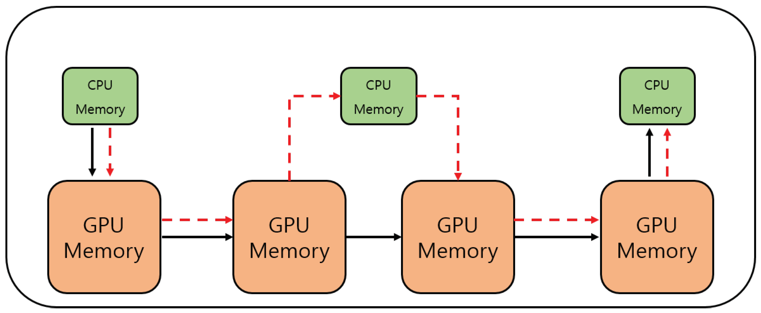
3.3. Data Transfer between the CPU and GPU

The objective of GPU-accelerated models is to shorten the time of numerical computation. Data transfer occurs between the CPU and GPU due to the difference in high-ware, and it should be programmed so that data transfer between them does not occur frequently. Therefore, the number of data transfers between the CPU and GPU should be reduced to a minimum, and the program should be implemented so that continuous operations are performed on the GPU. Figure 5 concisely shows the program system of the GPU-accelerated model developed in this study. Figure 6 shows a part of the code for the CUDA Fortran numerical computations part of Figure 2. Data transfer between CPU and GPU was performed only in rows 1 and 11 to minimize the number of transfers. Lines 3 to 7 are instructions for the continuous operation of the GPU. However, the GPU-accelerated Laplace equation model does not run continuously on the GPU. As shown in Figure 5 and Figure 6 in lines 2 and 8 to 10, it is programmed so that GPU operation is temporarily suspended due to CPU operation while GPU operation is being performed. Then, GPU operation is performed again after the CPU operation is completed. Such a cause is judged to be the limitation of the function command of the CUDA program.

4. Numerical Cases and Results

4.1. Comparison of the Numerical Result and the Analysis Solution

The accuracy of the GPU-accelerated Laplace equation model was analyzed by comparing the result, from the numerical simulation and analytical solution for Equations (13a) and (13b), which are publicly known.

$$\begin{array}{c}\hfill \begin{array}{c}\hfill {\displaystyle \frac{{\partial }^2\varphi }{\partial x^2}}+{\displaystyle \frac{{\partial }^2\varphi }{\partial y^2}}=0,0<x<a,0<y<b\end{array}\end{array}$$

(13a)

$$\begin{array}{c}\hfill \begin{array}{c}\hfill \left\{\begin{array}{c}\varphi (0,y)=0\hfill \\ \varphi (a,y)=0\hfill \\ \varphi (x,0)=0\hfill \\ \varphi (x,b)=f\left(x\right),\hfill \end{array}\right.\end{array}\end{array}$$

(13b)

where x and y are the horizontal and vertical axes, $\varphi$ is the dimensionless temperature, a and b are arbitrary constants. The analytical solutions for Equations (13a) and (13b) are the same as those for Equation (14) [14].

$$\varphi (x,y)=\sum _{n=1}^{\infty }{A}_{n}sinh{\displaystyle \frac{n\pi }{a}}ysin{\displaystyle \frac{n\pi }{a}}x,$$

(14)

where $A_n$ is Equation (15), and in the case of $f\left(x\right)=100,a=1,b=1,A_n$ becomes Equation (16).

$$A_n={\displaystyle \frac{2}{asinh{\displaystyle \frac{n\pi b}{a}}}}{\int }_0^{a}f\left(x\right)sin{\displaystyle \frac{n\pi }{a}}xdx$$

(15)

$$A_n=200{\displaystyle \frac{1-{(-1)}^n}{n\pi sinhn\pi }}.$$

(16)

In the numerical tests, numerical grids the size of $0.05\times 0.05$ were applied. Figure 7 shows the numerical model and the analytical solution result, and the two results agree well. The Normalized Root Mean Square Error (NRMSE) of the numerical analysis and analytical solution results was calculated and presented. For NRMSE, Equation (17) was used.

$$\mathrm{NRMSE}=\sqrt{{\displaystyle \frac{1}{m}}\sum _{k=1}^m{\left({\displaystyle \frac{A_k-F_k}{A_k}}\right)}^2},$$

(17)

where m is the number of numerical analysis result values, $A_k$ is the analysis result value, and $F_k$ is the numerical analysis result value. The NRMSE for Figure 7 is $3.9\times {10}^{-4}$, which indicates that the numerical analysis result of the GPU-accelerated Laplace equation and the analysis solution agree well.

4.2. Groundwater Flow around Sheet Pile Dam

The velocity potential and stream function were obtained by applying the GPU-accelerated Laplace equation model to a sheet pile dam, which is often used as a benchmark for groundwater flow. Figure 8 is a cross-sectional view of the sheet pile dam. The upstream water depth is 2 m, the downstream water depth is $0.5$ m, and the sheet piles are located up to 15 m deep in the soil layer. The impermeable layer is just below the soil layer.

Figure 9a,b shows the boundary conditions for finding the velocity potential and the stream function. Dirichlet boundary conditions and Neumann boundary conditions were applied. Section 1 to Section 9 are Dirichlet boundary conditions. Section 1 is $\varphi =2.0$ m, Section 2 is $\varphi =0.5$ m, Section 3 is $\varphi =0$ m, Section 4 to Section 6 is $\psi =0.5$ m${}^2$/s, and Section 7 to Section 9 is $\psi =2.0$ m${}^2$/s.

Figure 10 is the numerical analysis result of the CPU-accelerated Laplace equation model. Figure 10a shows the mesh configuration for the computational domain. Figure 10b shows the equipotential line by finding the velocity potential, and Figure 10c shows the streamline by finding the stream function. As a result of applying the GPU-accelerated Laplace equation model to the sheet pile dam, it was confirmed that the equipotential line and the streamline were approximately perpendicular to each other as shown in Figure 10d. This indicates that the GPU-accelerated Laplace equation model represents the groundwater flow around the sheet pile dam relatively well.

4.3. Irregular Calculation Area

In order to apply the GPU-accelerated Laplace model to the irregular calculation area, a sector-shaped calculation area, as shown in Figure 11, was set.

Where $RW=RZ=0.1m$, $RX=RY=1m$ and the angle between $RX$ and $RY$ is 90 degrees. Dirichlet boundary conditions were applied as boundary conditions for the computational domain, and the value is the same as Equation (18).

$$\left\{\begin{array}{c}\begin{array}{cccc}\hfill \varphi & =0\hfill & & atWX\\ \hfill \varphi & ={\displaystyle \frac{sin\theta }{r_{XY}}}\hfill & & atXY\\ \hfill \varphi & ={\displaystyle \frac{1}{r_{YZ}}}\hfill & & atYZ\\ \hfill \varphi & ={\displaystyle \frac{sin\theta }{r_{WZ}}}\hfill & & atZW\end{array}\hfill \end{array}\right.$$

(18)

The numerical computation results of GPU-accelerated Laplace equations were verified by comparing them with the CPU-based numerical analysis results preceded by Fletcher [12]. Figure 12 shows the results of calculating the velocity potential using the GPU-accelerated Laplace equation model for various numbers of grids. The NRMSE for Figure 12a and the numerical analysis results of the GPU-accelerated Laplace equation and the numerical analysis results of the CPU-based Laplace equation by Fletcher [12] agree well. The result of calculating the velocity potential by increasing the number of grids from Figure 12b–d showed a similar trend to that of Figure 12a.

4.4. Performance of GPU-Accelerated Laplace Equation Models

The performance of the GPU-accelerated Laplace equation model for computational execution time was compared by measuring the overall program execution time of each GPU- and CPU-based Laplace equation model for the results of Figure 13. The GPU-accelerated numerical model and the CPU-based numerical model assumed the same algorithm. Speedup, a measure of the performance improvement of parallel computers, was used for the performance of the calculation time. The speedup is the same as Equation (19).

$$Speedup={\displaystyle \frac{CPUtime}{GPUtime}},$$

(19)

where GPU time is the overall program execution time of the GPU-accelerated numerical model, and is the overall program execution time of the CPU-based numerical model. The relationship between the number of grids and the speedup was confirmed by variously configuring the number of grids in the calculation area. As shown in Figure 13, the number of grids increased from $1.0\times {10}^4$ to $4.0\times {10}^6$, and as the number of grids increased, the speedup also increased. An increase in the number of grids is associated with an increase in the data to be processed. As the number of data increases, the numerical simulation time increases. As the number of grids increases, the performance of the model tends to increase the efficiency of GPU parallel processing. As a result, the GPU-accelerated Laplace equation model shortened the computation time by up to 50 times compared to the CPU-based Laplace equation model. It is judged that, when a large-scale operation is performed, the use of a GPU can shorten the operation time compared to using only one CPU.

In the developed model, some data operations are being performed on the CPU due to the limitations of the functions provided by CUDA Fortran. To obtain higher acceleration results, the model must be programmed so that most data operations are performed on the GPU.

5. Conclusions

In this study, in order to shorten the computational execution time for the numerical analysis of Laplace equations, a GPU-accelerated Laplace equation model was implemented to verify the accuracy of the numerical analysis results and to confirm the performance of the computational execution time. The GPU-accelerated Laplace equation model applied a technique called CUDA and implemented the use of the Fortran language. As a way to shorten the computation time by applying CUDA technology, large-scale parallel computations were performed on the GPU, and a program was written to reduce the number of data transfers between the CPU and GPU.

The results of the GPU-accelerated Laplace equation model were in good agreement with the analytical solution and the results of previous studies. As for the computational execution time performance of the model, the performance increased as the number of grids increased. When the number of grids was $4.0\times {10}^6$, the time was shortened by up to about 50 times. When performing large-scale calculations, the performance of the GPU-accelerated Laplace equation model with respect to time is higher than the computation execution time of the existing CPU-based numerical model. We conclude from these results that the GPU-accelerated Laplace equation model can be applied to the research of groundwater flows targeting large areas.

Although this study provides an early stage for the GPU-based Laplace equation model, several areas of development are still needed. Various algorithms will be developed for the CUDA Fortran library. If most of the data processing is performed on the GPU, there is room for a further reduction in simulation execution time. In addition, the developed model should be studied on optimization. If the performance of CUDA is improved, it is judged that the performance of the CUDA Fortran-based model will also be further improved.

References

1. Harju, A.; Siro, T.; Canova, F.F.; Hakala, S.; Rantalaiho, T. Computational physics on graphics processing units. In International Workshop on Applied Parallel Computing; Springer: Berlin/Heidelberg, Germany, 2012; pp. 3–26. [Google Scholar]
2. Chow, A.D.; Rogers, B.D.; Lind, S.J.; Stansby, P.K. Incompressible SPH (ISPH) with fast Poisson solver on a GPU. Comput. Phys. Commun. 2018, 226, 81–103. [Google Scholar] [CrossRef]
3. NVIDIA. Cuda c Programming Guide; Version 4.0; NVIDIA Corporation: Santa Clara, CA, USA, 2011. [Google Scholar]
4. Munshi, A.; Gaster, B.; Mattson, T.G.; Ginsburg, D. OpenCL Programming Guide; Pearson Education: London, UK, 2011. [Google Scholar]
5. Vanderbauwhede, W.; Takemi, T. An investigation into the feasibility and benefits of gpu/multicore acceleration of the weather research and forecasting model. In Proceedings of the 2013 International Conference on High Performance Computing & Simulation (HPCS), Helsinki, Finland, 1–5 July 2013; pp. 482–489. [Google Scholar]
6. Bae, S.K. Acceleration of Word2vec Using GPUs. Master’s Thesis, University of Seoul, Seoul, Korea, 2017. [Google Scholar]
7. Gomez Gesteira, M.; Crespo, A.J.; Rogers, B.D.; Dalrymple, R.A.; Dominguez, J.M.; Barreiro, A. Sphysics—Development of a freesurface fluid solver—Part 2: Efficiency and test cases. Comput. Geosci. 2012, 48, 300–307. [Google Scholar] [CrossRef]
8. Gomez Gesteira, M.; Rogers, B.D.; Crespo, A.J.; Dalrymple, R.A.; Narayanaswamy, M.; Dominguez, J.M. Sphysics—Development of a free-surface fluid solver—Part 1: Theory and formulations. Comput. Geosci. 2012, 48, 289–299. [Google Scholar] [CrossRef]
9. Afrasiabi, M.; Klippel, H.; Röthlin, M.; Wegener, K. An improved thermal model for SPH metal cutting simulations on GPU. Appl. Math. Model. 2021, 100, 728–750. [Google Scholar] [CrossRef]
10. Kim, Y.T.; Lee, Y.L.; Chung, K.Y. WRF Physics Models Using GP-GPUs with CUDA Fortran. Korean Meteorol. Soc. 2013, 23, 231–235. [Google Scholar] [CrossRef] [Green Version]
11. Chang, T.K. Efficient Computation of Compressible flow by Higher-Order Method Accelerated Using GPU. Master’s Thesis, Seoul National University, Seoul, Korea, 2014. [Google Scholar]
12. Fletcher, C. Computational Techniques for Fluid Dynamics 1; Springer: New York, NY, USA, 1988; pp. 98–116. [Google Scholar]
13. Kim, B. Development of GPU-Accelerated Numerical Model for Surface and Ground Water Flow. Ph.D. Thesis, University of Seoul, Seoul, Korea, 2019. [Google Scholar]
14. Zill, D.; Wright, W.S.; Cullen, M.R. Advanced Engineering Mathematics; Jones & Bartlett Learning: Burlington, MA, USA, 2011; pp. 564–566. [Google Scholar]
Figure 1. Finite volume for a distorted grid [12].
Water 13 03435 g001
Figure 2. Flowchart for numerical scheme.
Water 13 03435 g002
Figure 3. Hardware architecture of the CPU and GPU [13].
Water 13 03435 g003
Figure 4. CUDA data processing flow [13].
Water 13 03435 g004
Figure 5. Program system of GPU-accelerated Laplace equation model; solid line: data transfer, dash line: task performance.
Water 13 03435 g005
Figure 6. CUDA program code.
Water 13 03435 g006
Figure 7. Comparison of analytical and numerical methods results for mesh configuration.
Water 13 03435 g007
Figure 8. Cross-section of sheet pile dam.
Water 13 03435 g008
Figure 9. Boundary conditions, solid line: Dirichlet boundary conditions, dash line: Neumann boundary conditions. (a) Velocity potential, (b) Stream function.
Water 13 03435 g009
Figure 10. Computed results of velocity potential and stream function for mesh configuration. (a) Mesh configuration, (b) Equipotential line, (c) Streamline, (d) Flow net.
Water 13 03435 g010
Figure 11. Computational domain for the solution of Laplace equation; number of grids: 24 × 24 .
Water 13 03435 g011
Figure 12. Computed velocity potential for various number of grids. (a) number of grids: 6 × 6 , (b) number of grids: 12 × 12 , (c) number of grids: 18 × 18 , (d) number of grids: 24 × 24 .
Water 13 03435 g012
Figure 13. Performance measurement of computation time of the GPU-accelerated Laplace equation model.
Water 13 03435 g013