Abstract
The spatial and temporal distribution of precipitation is of great importance for the rain-fed agricultural production and the socioeconomics of Mato Grosso (MT), Brazil. MT has a sparse network of ground rain gauges that limits the effective use of precipitation information for sustainable agricultural production and water resources in the region. Several gridded precipitation products from remote sensing and reanalysis of land surface models are currently available that can enhance the use of such information. However, these products are available at different spatial and temporal resolutions which add some challenges to stakeholders (users) to identify their appropriateness for specific applications (e.g., irrigation requirements, length of growing season, and drought monitoring). Thus, it is necessary to provide an assessment of the reliability of these precipitation estimates. The objective of this work was to compare regional precipitation estimates over MT as provided by the Global Land Data Assimilation (GLDAS), Modern-Era Retrospective Analysis for Research and Applications (MERRA), Tropical Rainfall Measurement Mission (TRMM), Global Precipitation Measurement (GPM), and the Global Precipitation Climatology Project (GPCP) with ground-based measurements. The comparison was conducted for the 2000–2018 period at eleven ground-based weather stations that covered different climate zones in MT using daily, monthly, and annual temporal resolutions. The comparison used the Pearson correlation index–r, Willmott index–d, root mean square error—RMSE, and the Wilks methods. The results showed GPM and GLDAS estimates did not differ significantly with the measured daily, monthly, and annual precipitation. TRMM estimates slightly overestimated daily precipitation by about 4.7% but did not show significant difference on the monthly and annual scales when compared with local measurements. The GPCP underestimated annual precipitation by about 7.1%. MERRA underestimated daily, monthly, and annual precipitation by about 22.9% on average. In general, all products satisfactorily estimated monthly precipitation, and most of them satisfactorily estimated annual precipitation; however, they showed low accuracy when estimating daily precipitation. The TRMM, GPM, GPCP, and GLDAS estimates had the highest performance, from high to low, while MERRA showed the lowest performance. The findings of this study can be used to support the decision-making process in the region in application related to water resources management, sustainability of agriculture production, and drought management.
1. Introduction
The state of Mato Grosso (MT) has the third largest territorial area among the Brazilian states [1]. The economy of Mato Grosso is strongly dependent on agrobusiness production [2,3]. The agricultural activities in the state is characterized by increased production of rain-fed pasture (for livestock) and soybean [4]. Within a 20-year period, cropland of soybean increased by about 275% [3]. Based on 2017 estimates, Mato Grosso was considered the largest producer of soybean as it accounted for ~28.9% of all production in Brazil. The sustainability rainfed agricultural production and water resources is therefore affected by the spatial and temporal distribution of precipitation [3,4]. Similarly, precipitation plays a key role in evaluating drought conditions [5], streamflow forecasting [6], and regional water balance [7]. In common, these activities require adequate knowledge of precipitation dynamics [4]. For agricultural production, monitoring precipitation is essential to characterize agricultural zoning, crop planting, irrigation depth (requirements), and harvesting periods in MT [8,9,10]. The precipitation in MT varies, on average, from 1200 to 2200 mm year−1 [8]. This spatial variation occurs due to the state’s geographical location in the central region of South America, where intertropical and extratropical systems interact [11].
The highest amounts of precipitation occur in the northern part of the state, followed by the central, eastern, and southern regions, and are associated with the development of equatorial fronts that emerges from the Amazon during the rainy season [8]. Winter precipitation is influenced by cold fronts that influence the dry season in the state [12]. In addition to macroscale phenomena, the biophysical characteristics of the surface, such as vegetation and geographic relief, also influence the distribution of precipitation in the state [8]. However, the current spatial distribution of the weather stations in Mato Grosso is not geographically representative of the entire extent of the state, and the accessibility to the data is also limited due to the high number of measurement failures from methodological, technical, and geographic issues [13].
Precipitation estimates in places where there is no weather station can be obtained using several other alternative methods, among them, reanalysis products such as those from the Global Land Data Assimilation (GLDAS) and the Modern-Era Retrospective Analysis for Research and Applications (MERRA), and remote sensing products such as those from the Tropical Rainfall Measurement Mission (TRMM), Global Precipitation Measurement (GPM), and the Global Precipitation Climatology Project (GPCP). However, these products have their own advantages and disadvantages. The reanalysis methods can provide precipitation estimates at relatively high spatial resolution and represent the precipitation processes in synoptic scale properly, but recent findings suggested that they tend to have a high level of uncertainty when mesoscale convective regimes occur [14]. On the other hand, remote sensing products provide relatively better estimates but their estimates can be affected by the characteristics of the terrestrial surface and the microphysics of clouds, which may confuse high-level (cold) cloud tops with precipitation occurrence [15].
The socioeconomic of Mato Grosso is dependent on providing highly accurate spatial and temporal distribution of precipitation. Taking advantage of the several currently available precipitation products, it is important to provide an assessment and improved understanding of how these products are able to represent the spatial and temporal variability precipitation in the region. The objective of this study was to compare the precipitation estimated by the GLDAS, MERRA, TRMM, GPM, and GPCP products with ground observations in Mato Grosso. The analysis evaluated the performance of these products at daily, monthly, and annual time scales as well as spatially over Mato Grosso. The remaining of this paper was organized to provide a description of the study area, data and methods of evaluation used, summary of obtained results, discussions of the observed spatiotemporal variability, and conclusions.
2. Materials and Methods
2.1. Study Area
The state of Mato Grosso has an area of 903,206,997 km2 and is in the Midwest region of Brazil (6° S, 19.45° S and 50.06° W, 62.45° W). It has an estimated population of 3,484,466 inhabitants, and a population density of 3.36 inhabitants per 1 km2 [1]. The state of Mato Grosso extends over three biomes: Amazon rainforest, savanna (Cerrado), and Pantanal. These ecosystems have two well-defined seasons (dry and rainy), in which the northern region has higher rainfall, followed by the central, eastern, and southern regions [11,12]. According to the Köppen classification, the climate in the northern region is considered an Am class (humid or sub-humid tropical climate). The climate in the central and southern regions is considered an Aw class (tropical climate, with dry winter) [16]. The climate of the state of Mato Grosso is controlled by tropical and subtropical large and mesoscale systems [11]. However, there is a local effect on precipitation. The uneven heating of the surface causes convective rain, especially during the wet season. Thus, relatively close locations (less than 5 km) may have precipitation events of different duration and intensity, or a precipitation event may occur in one region and not in another. The (Padre Ricardo Remetter) PRR region is rural, while (Cuiabá) CBA is urbanized, leading to the occurrence of more frequent convective rains in PRR than in CBA. Thus, the daily and monthly average precipitation in PRR is higher than in CBA. The annual average of precipitation in PRR and CBA are statistically similar because, in this temporal scale, the large and mesoscale tropical and subtropical systems prevail over the local convection.
2.2. Precipitation Observations
Precipitation measurements were available for the period between 2000 and 2018 at eleven conventional weather stations (Table 1) as obtained from the Instituto National de Meteorologia (INMET) through the Meteorological Database for Education and Research (BDMEP) [17]. These stations are installed in the municipalities of Cáceres (CCR), Canarana (CNR), Cuiabá (CBA), Diamantino (DMT), Gleba Celeste (GBC), Matupá (MTP), Nova Xavantina (NVX), Padre Ricardo Remetter (PRR), Poxoréu (PXR), Rondonópolis (RDP), and São José do Rio Claro (SJRC). The spatial distribution of these weather station is shown in Figure 1. These 11 stations were selected because they provided more consistent long-term measurements with minimal number of missing observations (less than 5–10%). Increased number of missing data makes the comparison at the monthly and annual time scale unrealistic. The highest temporal resolution of these measurements was a daily time scale; thus, the data did not allow to compare precipitation at the sub-daily time scale.

Table 1.
Available data from conventional weather stations, including Cáceres (CCR), Canarana (CNR), Cuiabá (CBA), Diamantino (DMT), Gleba Celeste (GBC), Matupá (MTP), Nova Xavantina (NVX), Padre Ricardo Remetter (PRR), Poxoréu (PXR), Rondonópolis (RDP), and São José do Rio Claro (SJRC), used to validate precipitation estimates for Global Land Data Assimilation (GLDAS), Modern-Era Retrospective Analysis for Research and Applications (MERRA), Tropical Rainfall Measurement Mission (TRMM), Global Precipitation Measurement (GPM), and the Global Precipitation Climatology Project (GPCP) products in the state of Mato Grosso, Brazil.
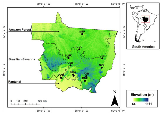
Figure 1.
Distribution of conventional weather stations in the state of Mato Grosso, Brazil along with the ground surface elevation and the distribution of the biomes (Amazon Forest, Brazilian Savanna, and Pantanal).
The distribution of weather stations does not homogenously represent the entire extent of the state for several reasons. One of the main reasons is the difficulty of geographic access. The southern part of the state is formed by the Pantanal which is the world’s largest floodplain, the northern region is formed by the Amazon rainforest and the northeast region is formed by a complex mosaic of indigenous lands (i.e., managed by native people). The locations of the weather stations have followed the state’s territorial occupation pattern since the 1970s.
The CBA and PRR stations are near each other with only 30 km apart. Thus, the pixels (the station location nearest to the center of the pixel) of the GLDAS, TRMM, and GPM products in these two stations are not the same, but the corresponding pixels of the MERRA and GPCP products related to these two stations can be the same. The precipitation measurements by these two stations were not averaged as they provided statistically different averages at the daily and monthly time scale.
2.3. Precipitation Estimates
Precipitation estimates based on the GLDAS, MERRA, TRMM, GPM, and GPCP products as summarized in Table 2 were obtained from Giovanni Platform of the National Aeronautics and Space Administration (NASA) (https://giovanni.gsfc.nasa.gov/giovanni/).

Table 2.
Spatial and temporal resolutions and versions of each of the precipitation products used over the state of Mato Grosso, Brazil.
The GLDAS uses global land surface models to generate (develop) near real time products land surface fluxes and states by ingesting (being forced by ground- and satellite-based data [18]). The main objective of the GLDAS was to develop terrestrial surface model outputs that preserve the climatological consistency [18]. Since its development, GLDAS has developed a number of versions with improved products based on Noah, VIC, Mosaic, and Catchment land surface models. In this study, out of the three components of the GLDAS version 2 (GLDAS 2.0, GLDAS 2.1, and GLDAS 2.2), precipitation estimates from GLDAS 2.1 Noah Model 3.6 was used. GLDAS 2.1 does not include the data assimilation process, combines mode and surface observations, and has 3 h and monthly products since 2000. The 3 h estimates were aggregated to daily time scale to match that of the measurements. It should be noted that the GLDAS 2.1 was the forces with the GPCP V1.3 daily precipitation fields between 2000–2001 and AGREMET since 2001.
The MERRA version 2 is a reanalysis of satellite observations projected conducted by the NASA Global Modeling and Assimilation Office (GMAO). MERRA uses the Goddard Earth Observing System Version 5 (GOES-5) model focusing on historic climate analysis, and its dataset provides precipitation estimates based on a large number of satellite observations and general circulation models [19,20] in combination with weather stations observation to parameterize initial conditions. Version 5.12.4 of MERRA-2 uses microwave and hyperspectral infrared measurements, and it is available at 1 h temporal resolution. The 1 h estimates were aggerated to daily time scale to match that of the measurements.
The TRMM Multi-Satellite Precipitation Analysis (TMPA) provided precipitation estimates by combining data from 3 sensors i.e., precipitation radar (PR), microwave imager (TMI), and visible and infrared (VIRS), as well as gauge observations [21]. TRMM era data is available from 1997 until 2019 as it seized operation in 2015. The science community transitioned to the GPM that was launched in 2014 with its improved precipitation product. The TRMM 3B42 v7 product was developed to maximize the quality of precipitation data for applied research in meteorology and hydrology globally [22]. It should be noted that more consistent TRMM 3B42 v7 data were the one available for the period between January 1998 to September 2014. After this period until December 2019, the 3B42 v7 algorithm was processed in parallel with GPM (IMERG). The TRMM data were available at the daily time scale—the same temporal resolution of that of the measurements.
The GPM is considered a successor of TRMM with enhanced rain and snow observation. The GPM Core Observatory was launched in February 2014 with Dual-Frequency Precipitation Radar (DPR) and GPM Microwave Imager (GMI) instruments [23] to create a global precipitation dataset [23]. The GPM has uses its Integrated Multi-Satellite Retrievals (IMERG) algorithm to develop a global precipitation dataset from a satellite constellation in collaboration with international members [23] (i.e., 6 passive microwave radiometers and 5 geosynchronous infrared sensors). The IMERG algorithm also fuses TRMM historic data (from 2000 to 2015) with the recent GPM (i.e., DPR and GMI) observations (from 2014 onward) to provide long-term precipitation dataset. The highest temporal resolution of GPM is 30 min and was accumulated and processed by the GES DISC to the daily time scale. It should be noted that while GPM and TRMM mostly use the same input datasets, their different algorithms used in producing these estimates allowed GPM to provide its high frequency precipitation values (30 min). This allows to capture the temporal evolution of precipitation events more accurately; thus, it is expected to obtain more accurate time-averaged daily values.
The GPCP is part of the Global Climate and Energy Exchange Project (GEWEX) of the World Climate Research Program (WCRP), to maintain homogeneous global record of long-term precipitation estimates and information for climate studies. GPCP, which has data available since 1983, is based on five dataset (i.e., passive microwave, IR, and gauges) mainly from geostationary satellites and surface measurements of precipitation [24]. One of these five datasets include TRMM Composite Climatology (TCC) which was developed to be used for global scale modeling such as GCM [25]. The highest temporal resolution to GPCP is the monthly time scale; thus, the measurements were aggregated to monthly in order to be compared with GPCP.
2.4. Performance Indicators
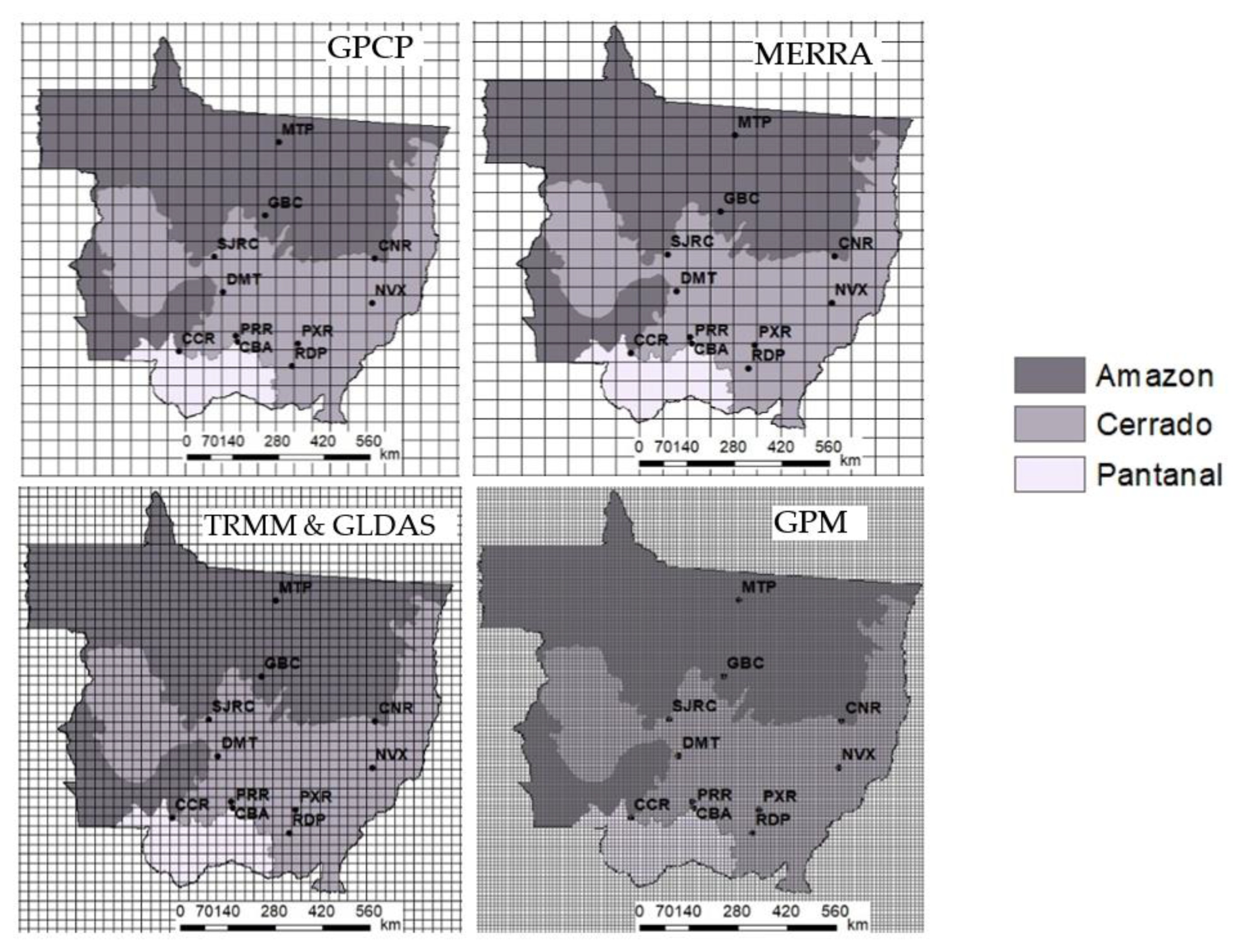
The daily, monthly, and annual precipitation estimates as provided by these different products were analyzed only when there were no data gaps in the corresponding observations from conventional weather stations. The geographic location of each weather stations was matched with a corresponding pixel (closest to the center of a pixel) of the gridded products (i.e., from remote sensing and reanalysis) (Figure 2). Direct comparison of point to pixel values allowed to preserve the integrity of the gridded precipitation estimates (without altering their values). Thus, no resampling or aggregation of the gridded data in terms of the spatial resolution was conducted since this also requires running all precipitation algorithms used to develop these products—which is beyond the scope of this analysis. Thus, the comparison of the gridded data with station data was conducted using their native spatial resolution.
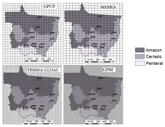
Figure 2.
Spatial representation of the weather stations locations and the grid resolution (as shown in Table 2) of the precipitation products.
The daily, monthly, and annual averages of precipitation values (both estimates and measurements) along with their respective confidence intervals (±95%) were calculated using a bootstrapping resampling technique with 1000 interactions. The bootstrap allows to estimate randomly repeated samples for a dataset of the same size as the original sample. The confidence interval indicates the reliability of an estimate. Based on this method, the obtained averages particularly of those of the measurements from nearby stations (i.e., CBA and PRR) are significantly different.
The correlation between measured and estimated precipitation values was evaluated using the Pearson correlation index—r, which indicates the degree of the agreement between two data sets (Equation (1)):
where is the estimated precipitation value (on daily, monthly, or annual time scale), i represents a numerator for the number of observations from 1 to n with n the total number (days, month, years). is the average of the estimated precipitation value, is the measured precipitation value, and is the average of the measured precipitation.
The agreement between observed and estimated precipitation was also assessed using the index of agreement—d (Equation (2)) as proposed by [26]. This index ranges from zero to one, representing non-agreement and perfect agreement, respectively [11]:
The analysis of the average error in precipitation estimates was assessed using the root mean square error (RMSE) (Equation (3)), where n is the number of observations. RMSE values close to zero is expected for reduced error and increased accuracy [11]:
The performance of the products in detecting daily precipitation events was evaluated using the Wilks method proposed by [27], which utilizes categorical indices (Equations (4)–(7)) that are based on the correctness or error criteria of the estimates relative to the measured values (Table 3).

Table 3.
Contingency table to assess the accuracy of the daily GLDAS, MERRA, TRMM, and GPM products in the state of Mato Grosso, Brazil. The table was not applied to GPCP since it does not provide estimates of daily precipitation.
The contingency table suggested that if a product indicated that there was (or was not) precipitation during a particular day, so as the measurements from a weather station, then this day can be accounted in category a (or d). Thus, the total number of days that were correctly assigned precipitation values (regardless of their accuracy) can be calculated. On the other hand, if a product indicated that there was (or was not) precipitation during a particular day but actually there was not (or was), based on measurements, then this day can be accounted in category b (or c).
The ratio (dimensionless) of occurrences of precipitation events to those that did not occur was obtained through the False Alarm Ratio (FAR) indicator, which has an ideal value of zero (Equation (4)):
The ability of a product to correctly (or not) precipitation events was determined by the Probability of Detection (POD) indicator (dimensionless ratio). POD values close to 1 indicate better model accuracy in predicting the precipitation event (Equation (5)):
The tendency of a precipitation product to overestimate or underestimate the total number of events (thus potentially the precipitation amounts) was determined by the BIAS (dimensionless) (Equation (6)), where BIAS = 1, BIAS > 1, and BIAS < 1 represent perfect agreement, overestimation, and underestimation, respectively:
The proportion in the number of correctly predicted precipitation events to the cases where there were no precipitation events was provided by Critical Success Index (CSI) indicator (dimensionless), with ideal value of 1 (Equation (7)):
In the validation of models of natural phenomena, it is necessary to determine if their behavior is similar to that of the observed. Thus, the Taylor diagram was used to concisely summarize the degree of correspondence between estimated and measured data [28]. Taylor diagram allows to visually presents descriptive statistical summary that include the standard deviation, correlation coefficient (r), and the RMSE [28].
3. Results
3.1. Assessment of Temporal Accuracy
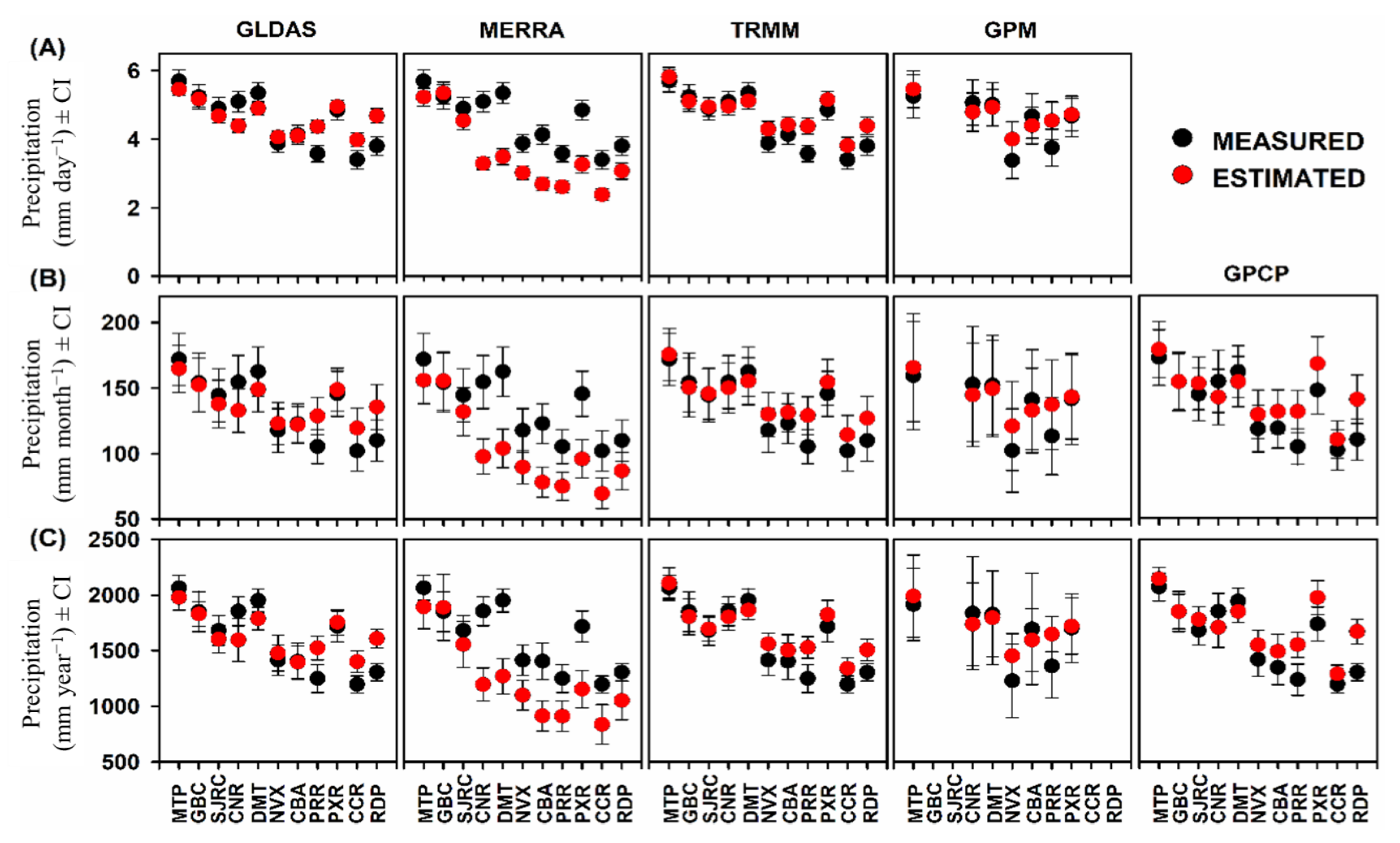
The daily precipitation estimates by the TRMM consistently overestimated the corresponding measurements by about 4.7%. Monthly and annual precipitation estimates by TRMM were not significant different from the corresponding measurements. Similarly, monthly precipitation estimates by the GPCP did not show significant difference when compared with measurements, however, the annual precipitation estimates overestimated the measurements by 7.1%. Precipitation estimates by MERRA consistently underestimated observations by an average of about 22.9% on the three-time scales (i.e., daily, monthly, and annual). The precipitation estimated by the GLDAS and GPM products did not differ significantly on all the three-time scales (daily, monthly, and annual) when compared with the measurements. A relatively similar performance by the TRMM was also observed at the monthly and annual precipitation estimates and by the GPCP at the monthly precipitation estimates (Figure 3).
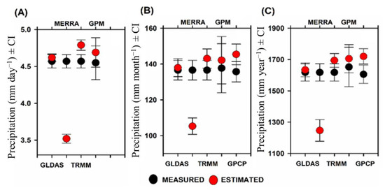
Figure 3.
Averages values with the corresponding ± Confidence Interval (CI) of (A) daily (mm day−1), (B) monthly (mm month−1), and (C) annual (mm year−1) precipitation as measured by conventional weather stations and estimated by GLDAS, MERRA, TRMM, GPM, and GPCP products in the state of Mato Grosso, Brazil. For (A), the daily values for the entire study period were averaged, while for (B), the monthly values for all months during the study period were averaged, and the annual values in (C) were the annual values averaged for all years during the study period.
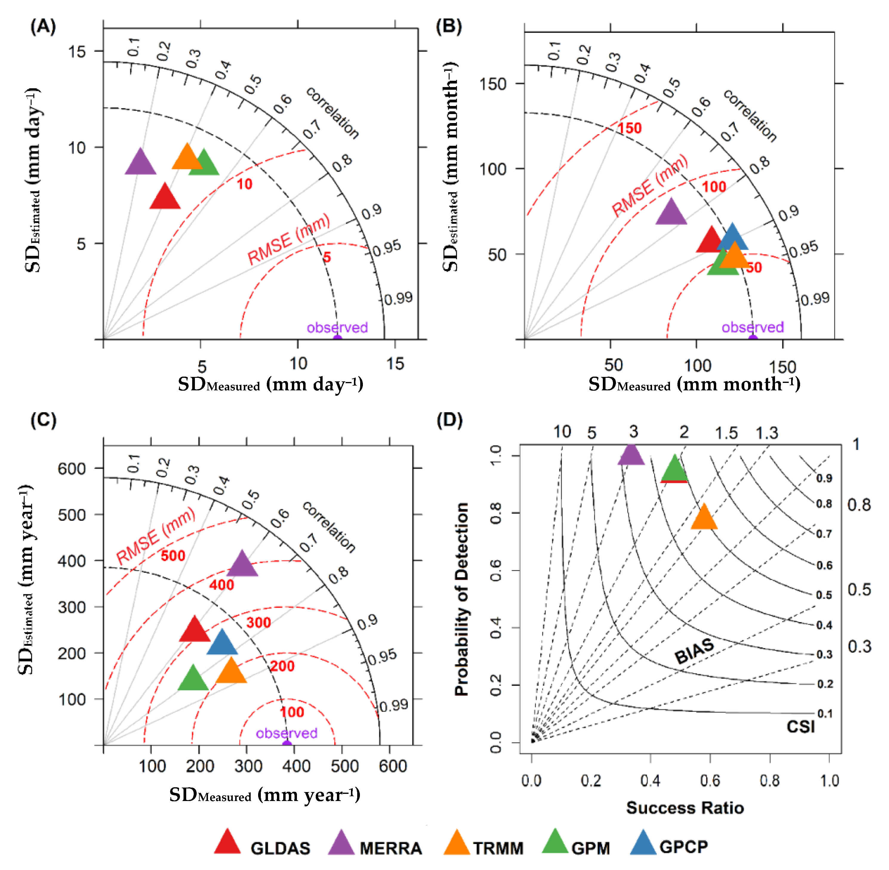
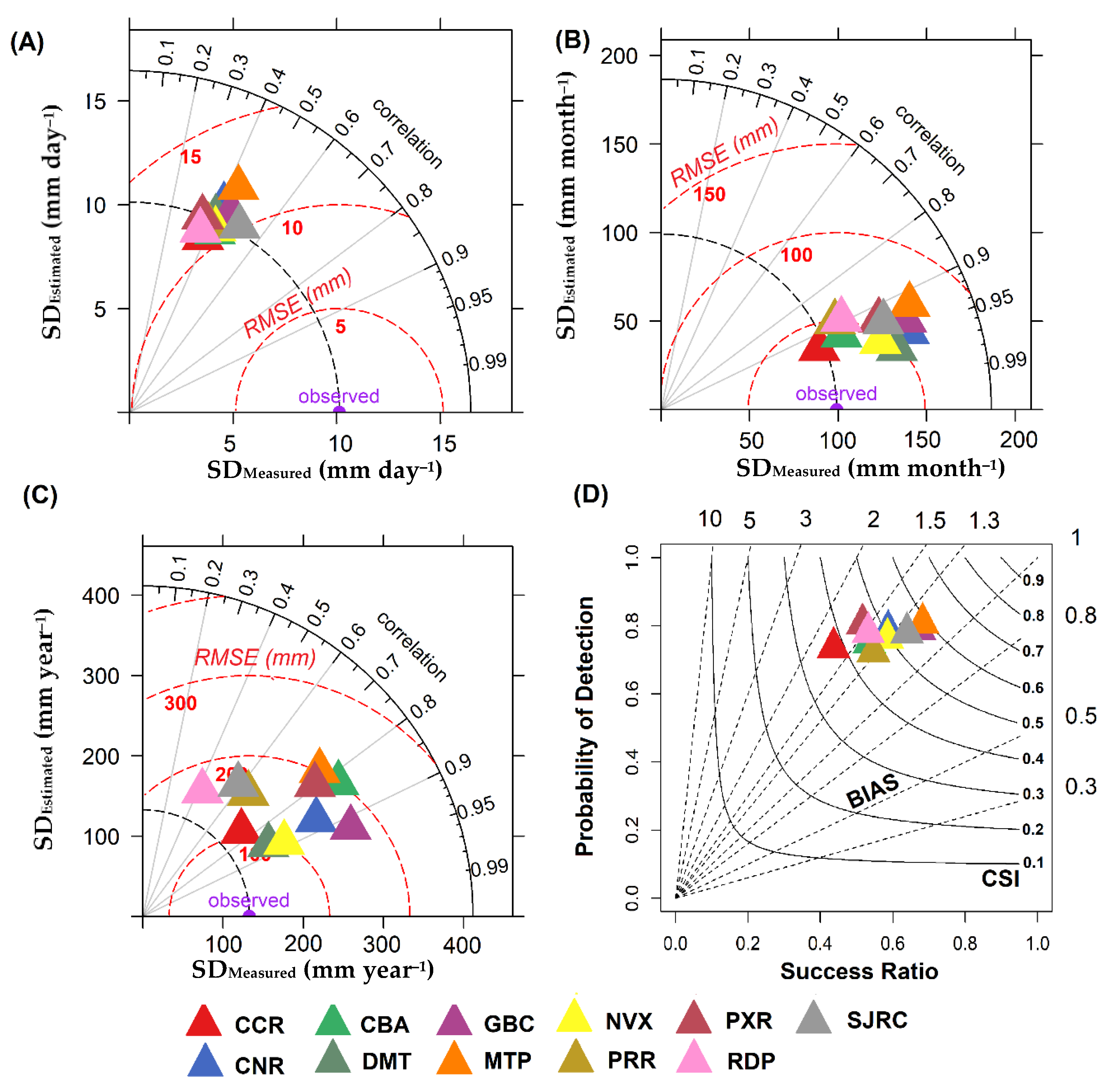
Daily precipitation estimates based on the GPM had the highest correlation and Willmott coefficients and the smallest error (r = 0.49; d = 0.68; and RMSE = 11.25 mm day−1) than those provided by all other products. On the other hand, the daily precipitation estimated by MERRA had lowest correlation and Willmott coefficients and highest error (r = 0.20; d = 0.35; and RMSE = 13.93 mm day−1) (Figure 4A).

Figure 4.
Taylor diagrams showing the comparisons of (A) daily (mm day−1), (B) monthly (mm month−1), (C) annual (mm year−1) measured and estimated precipitation as well as (D) the performance diagram of GLDAS, MERRA, TRMM, GPM, and GPCP products in the state of Mato Grosso, Brazil. In panels A, B, and C, the Pearson correlation coefficient (r) is represented by the azimuth angle (black outlines), the Root Mean Square Error (RMSE) is represented by the red dashed outlines, and the standard deviation (SD) was indicated on the x and y axes, respectively. In panel D, the probability of detection (POD) is represented on the x and y axes; the BIAS was indicated by the dashed black lines; and the critical success index (CSI) is represented by continuous black lines. For (A), the daily values for the entire study period were averaged, while for (B), the total monthly values for all months during the study period were averaged, and the annual values in (C) were the annual values averaged for all years during the study period.
The monthly precipitation estimates by the GPM resulted in r = 0.93; d = 0.96; and RMSE = 45.26 mm month−1 and those by the TRMM resulted in r = 0.93; d = 0.96; and RMSE = 48.75 mm month−1. Both GPM and TRMM monthly estimates had higher correlation and Willmott coefficients and smaller error than those provided by the other three products (i.e., MERRA, GLDAS, GPCP). The monthly precipitation estimated by MERRA resulted in the lowest correlation and Willmott coefficients and the highest error with r = 0.76; d = 0.84; and RMSE = 92.40 mm month−1 (Figure 4B).
On an annual time scale, the performance of precipitation estimates from all products was similar to that of the monthly time scale, with highest correlation and Willmott coefficients and the lowest error provided by the GPM (r = 0.86; d = 0.90; and RMSE = 207.98 mm year−1) and TRMM (r = 0.80; d = 0.86; and RMSE = 198.44 mm year−1) (Figure 4C).
Based on the Wilks performance indicators (Equations (4)–(7)), the daily precipitation estimates by the TRMM provided the best performance as indicated by the categorical indices with CSI = 0.49, POD = 0.57, and FAR = 0.22. However, the daily products by the GPM, TRMM, GLDAS, and MERRA tended to underestimate the occurrence of daily precipitation events, with a BIAS that ranged from 0.33 to 0.74. MERRA persistently provided an occurrence of daily precipitation events and resulted in CSI = 0.33, POD = 0.33, FAR = 0, indicating that it estimated a high number of events on days when, in reality, there were no daily precipitation events (Figure 4D).
3.2. Spatial Variability
Generally, the performance of the daily, monthly, and annual precipitation estimated by the GPM in all locations did not significantly differ from the measurements. The GLDAS underestimated daily precipitation in CNR by about 14% and overestimated daily and annual precipitation in PRR (21%), CCR (17%), and RDP (23%). The TRMM overestimated daily precipitation in PRR (22%) and RDP (15%). The GPCP overestimated annual precipitation in PRR (25%) and RDP (28%). The MERRA product underestimated daily, monthly, and annual precipitation from 19.3% to 35.4% in all but three stations that include MTP, GBC, and SJRC, where there was no significant difference when compared with the measurements (Figure 5). The performance of individual precipitation products in terms of spatial variability was detailed below.

Figure 5.
Average values with the corresponding ± Confidence Interval (CI) of (A) daily (mm day−1), (B) monthly (mm month−1), and (C) annual (mm year−1) precipitation as measured by conventional weather stations and estimated by the GLDAS, MERRA, TRMM, GPM, and GPCP products in the state of Mato Grosso, Brazil. For (A), the daily values for the entire study period were averaged, while for (B), the total monthly values for all months during the study period were averaged, and the annual values in (C) were the annual values averaged for all years during the study period.
3.2.1. GLDAS
The daily precipitation estimates by GLDAS had the highest correlation and Willmott coefficients in GBC with r = 0.46 and d = 0.62 and the lowest in PRR with r = 0.35 and d = 0.55. The highest RMSE was obtained with the daily precipitation estimates in MTP with an RMSE of 12.88 mm day−1 and the lowest was in CCR (RMSE = 10.05 mm day−1) (Figure 6A). The monthly precipitation estimates had highest correlation and Willmott coefficients in GBC (r = 0.92 and d = 0.96) and the lowest, but significant, in CBA (r = 0.82 and d = 0.90). The highest error in the monthly precipitation estimates was obtained in CRR with an RMSE = 75.12 mm month−1 and the smallest was in CCR (RMSE = 53.83 mm month−1) (Figure 6B). The annual precipitation estimates showed higher variability in the correlation and Willmott coefficients in different locations, with the highest values of r = 0.89 and d = 0.88 and the lowest error of RMSE = 100.51 mm year−1 obtained in GBC (Figure 6C).
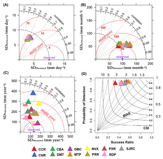
Figure 6.
Taylor diagrams showing the comparisons of (A) daily (mm day−1), (B) monthly (mm month−1), and (C) annual (mm year−1) measured and estimated precipitation, as well as (D) the performance diagram of the GLDAS product at each of the weather stations in the state of Mato Grosso, Brazil. In panels (A–C), the Pearson correlation coefficient (r) is represented by the azimuth angle (black outlines), the RMSE was represented by the red dashed outlines, and the standard deviation (SD) was indicated by the x and y axes, respectively. In panel (D), the probability of detection (POD) is represented on the x and y axes; the BIAS was indicated by the dashed black lines; and the critical success index (CSI) is represented by continuous black lines. For (A), the daily values for the entire study period were averaged, while for (B), the total monthly values for all months during the study period were averaged, and the annual values in (C) were the annual values averaged for all years during the study period.
The daily precipitation estimated by GLDAS in MTP had the highest performance as indicated by the categorical indicators with CSI = 0.55, FAR = 0.04%, BIAS = 0.59, and POD = 0.57). It was noticed that the resulted categorical indices tended to decrease with increasing latitude, until reaching the lowest values in CCR of CSI = 0.32, POD = 0.32, FAR = 0.06, and BIAS = 0.35) (Figure 6D).
3.2.2. MERRA
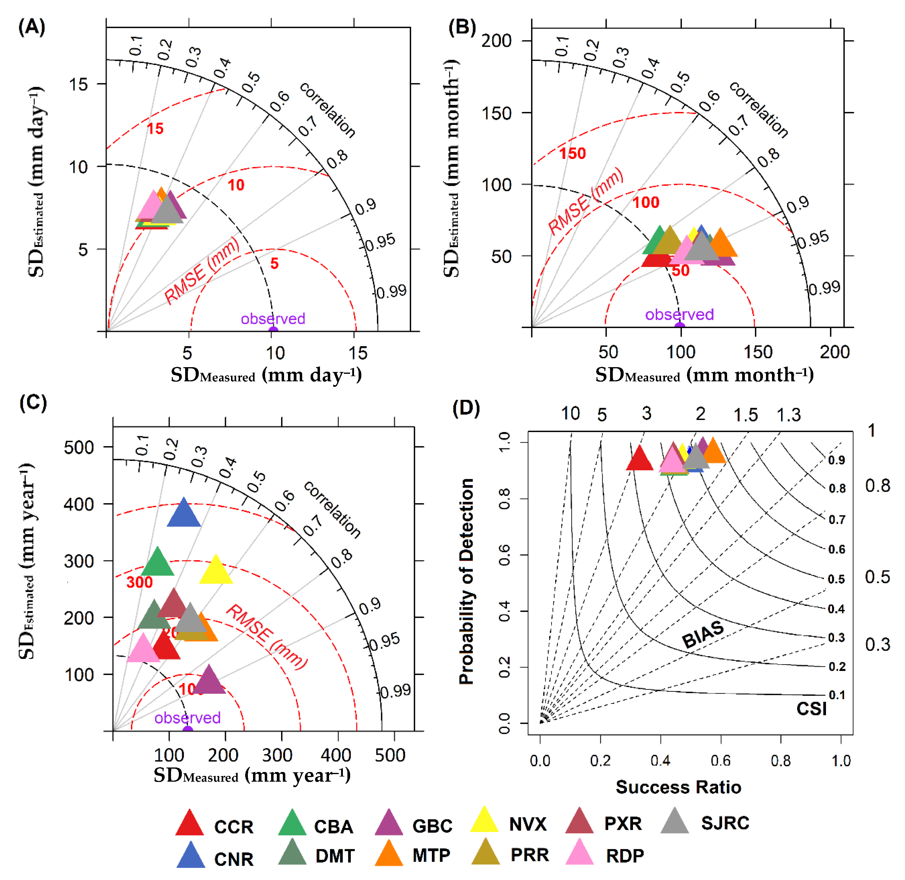
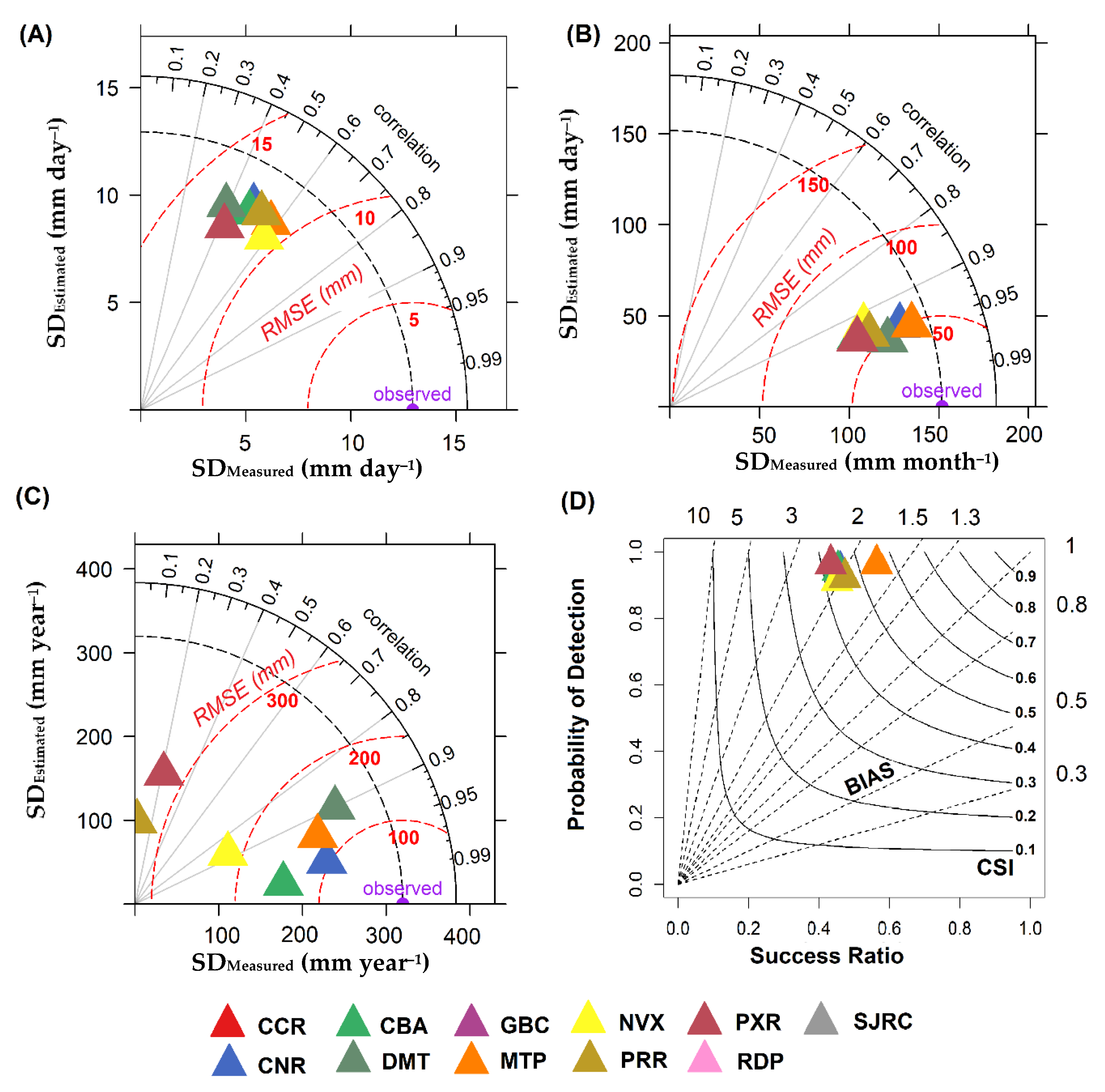
The daily precipitation estimates by MERRA had the highest correlation and Willmott coefficients in CNR (r = 0.24 and d = 0.43). The highest and smallest errors in the daily precipitation estimates were obtained in GBC (RMSE = 16.11 mm day−1) and in CCR (RMSE = 11.07 mm day−1) (Figure 7A). The monthly precipitation had the highest correlation in CNR (r = 0.82) and the highest Willmott coefficients in MTP and GBC with both had d = 0.87. The smallest error in monthly precipitation estimates was obtained in PRR (RMSE = 71.60 mm month−1) (Figure 7B). The annual precipitation estimates did not show any significant correlation in DMT and SJRC, had the highest correlation coefficients in CBA (r = 0.78), and the highest error in MTP (RMSE = 355.65 mm year−1) (Figure 7C).
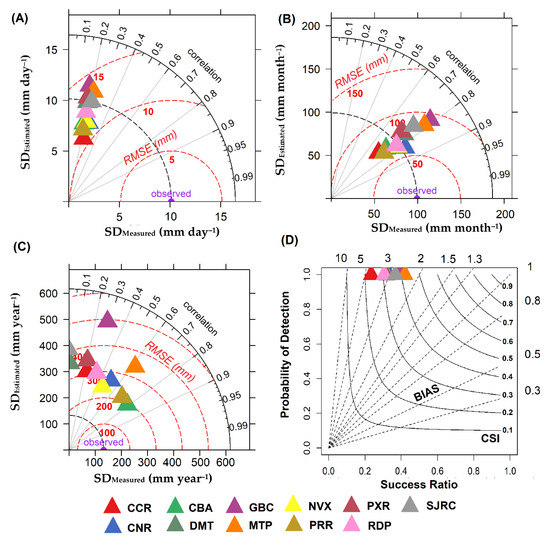
Figure 7.
Taylor diagrams showing the comparisons of (A) daily (mm day−1), (B) monthly (mm month−1), and (C) annual (mm year−1) measured and estimated precipitation, as well as (D) the performance diagram of the MERRA product at each of the weather stations in the state of Mato Grosso, Brazil. In panels (A–C), the Pearson correlation coefficient (r) is represented by the azimuth angle (black outlines), the RMSE was represented by the red dashed outlines, and the standard deviation (SD) was indicated by on the x and y axes, respectively. In panel (D), the probability of detection (POD) is represented on the x and y axes; the BIAS was indicated by the dashed black lines; and the critical success index (CSI) was represented by continuous black lines. For (A), the daily values for the entire study period were averaged, while for (B), the total monthly values for all months during the study period were averaged, and the annual values in (C) were the annual values averaged for all years during the study period.
The daily precipitation estimates by the MERRA in MTP showed the highest performance in detecting precipitation events as indicated by the categorical indices with CSI = 0.42, FAR = 0, and BIAS = 0.42. The lowest performance was shown in CCR with CSI = 0.23, FAR = 0, and BIAS = 0.23. Apparently, MERRA had consistently estimated the occurrence of precipitation events as indicated with the high values of probability of occurrence (Figure 7D).
3.2.3. TRMM
The daily precipitation estimates by the TRMM had the highest correlation and Willmott coefficients in SJRC (r = 0.51 and d = 0.69), and the lowest in PXR (r = 0.35 and d = 0.57). The lowest error in daily precipitation estimates was obtained in CCR (RMSE = 10.69 mm day−1) and the largest was obtained in MTP (RMSE = 13.72 mm day−1) (Figure 8A). The monthly precipitation estimates had the highest performance in DMT (r = 0.96; d = 0.98; and RMSE = 36.89 mm month−1) and the lowest (i.e., highest error) in PRR (RMSE = 54.84 mm month−1) (Figure 8B). The annual precipitation estimates had the highest correlation and Willmott coefficients and the lowest error in GBC (r = 0.91; d = 0.94; and RMSE = 136.26 mm year−1), the lowest correlations and highest errors in RDP (r = 0.42; d = 0.59; and RMSE = 259.37 mm year−1) and PRR (r = 0.79; d = 0.85; and RMSE = 341.44 mm year−1) (Figure 8C).
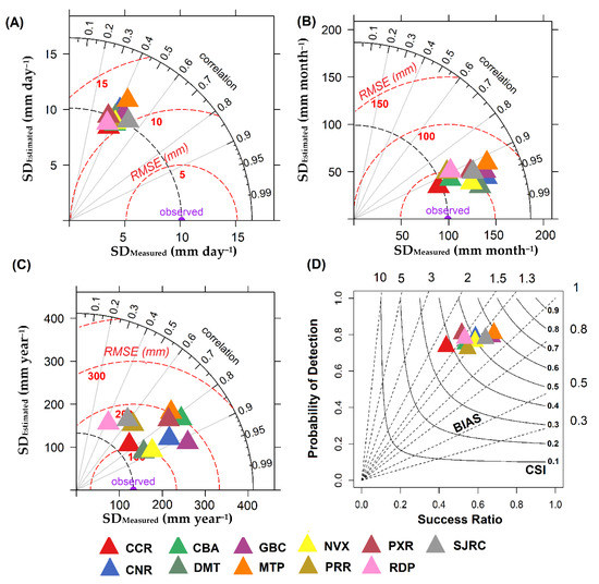
Figure 8.
Taylor diagrams showing the comparisons of (A) daily (mm day−1), (B) monthly (mm month−1), and (C) annual (mm year−1) measured and estimated precipitation, as well as (D) the performance diagram of the TRMM product at each of the weather stations in the state of Mato Grosso, Brazil. In panels (A–C), the Pearson correlation coefficient (r) was represented by the azimuth angle (black outlines), the RMSE was represented by the red dashed outlines, and the standard deviation (SD) was indicated by the x and y axes, respectively. In panel (D), the probability of detection (POD) is represented on the x and y axes; the BIAS was indicated by the dashed black lines; and the critical success index (CSI) was represented by continuous black lines. For (A), the daily values for the entire study period were averaged, while for (B), the total monthly values for all months during the study period were averaged, and the annual values in (C) were the annual values averaged for all years during the study period.
The daily precipitation estimates showed the highest performance in detecting the occurrence of daily events in MTP as indicated by the categorical indices (CSI = 0.58; POD = 0.68; and FAR = 0.19), and the lowest performance in CCR (CSI = 0.37; POD = 0.43; and FAR = 0.26). In addition, the BIAS indicated that the TRMM underestimated the occurrence of precipitation events with BIAS values ranged from 0.59 to 0.85 (Figure 8D).
3.2.4. GPM
The daily precipitation estimates by the GPM had the highest correlation and Willmott coefficients and the lowest error in NXV (r = 0.59; d = 0.75; and RMSE = 9.17 mm day−1). The lowest correlation coefficients and the highest error in DMT (r = 0.39; d = 0.59; and RMSE = 12.74 mm day−1) (Figure 9A). In contrast, the monthly precipitation estimates had the highest correlation and Willmott coefficients with error in DMT (r = 0.95; d = 0.97; and RMSE = 37.35 mm month−1) (Figure 9B). The annual precipitation estimates had the highest correlation and Willmott coefficients in CBA (r = 0.99 and d = 0.87) and DMT (r = 0.90 and d = 0.94), and the lowest ones in PRR (r = 0.02) and PXR (r = 0.21) (Figure 9C).
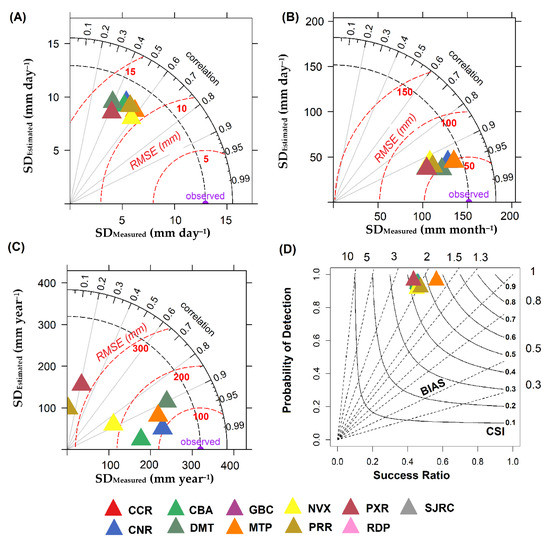
Figure 9.
Taylor diagrams showing the comparisons of (A) daily (mm day−1), (B) monthly (mm month−1), and (C) annual (mm year−1) measured and estimated precipitation, as well as (D) the performance diagram of the GPM product at each of the weather stations in the state of Mato Grosso, Brazil. In panels (A–C), the Pearson correlation coefficient (r) was represented by the azimuth angle (black outlines), the RMSE was represented by the red dashed outlines, and the standard deviation (SD) was indicated by the x and y axes, respectively. In panel (D), the detection probability (POD) is represented on the x and y axes; the BIAS was indicated by the dashed black lines; and the critical success index (CSI) was represented by continuous black lines. For (A), the daily values for the entire study period were averaged, while for (B), the total monthly values for all months during the study period were averaged, and the annual values in (C) were the annual values averaged for all years during the study period.
The best performance of the GPM in detecting the occurrence of daily precipitation events was in MTP as indicated by the categorical indices with CSI = 0.55, FAR = 0.03, BIAS = 0.58, and POD = 0.56 and the lowest was in PXR (CSI = 0.42, POD = 0.43, FAR = 0.03, and BIAS = 0.44) (Figure 9D).
3.2.5. GPCP
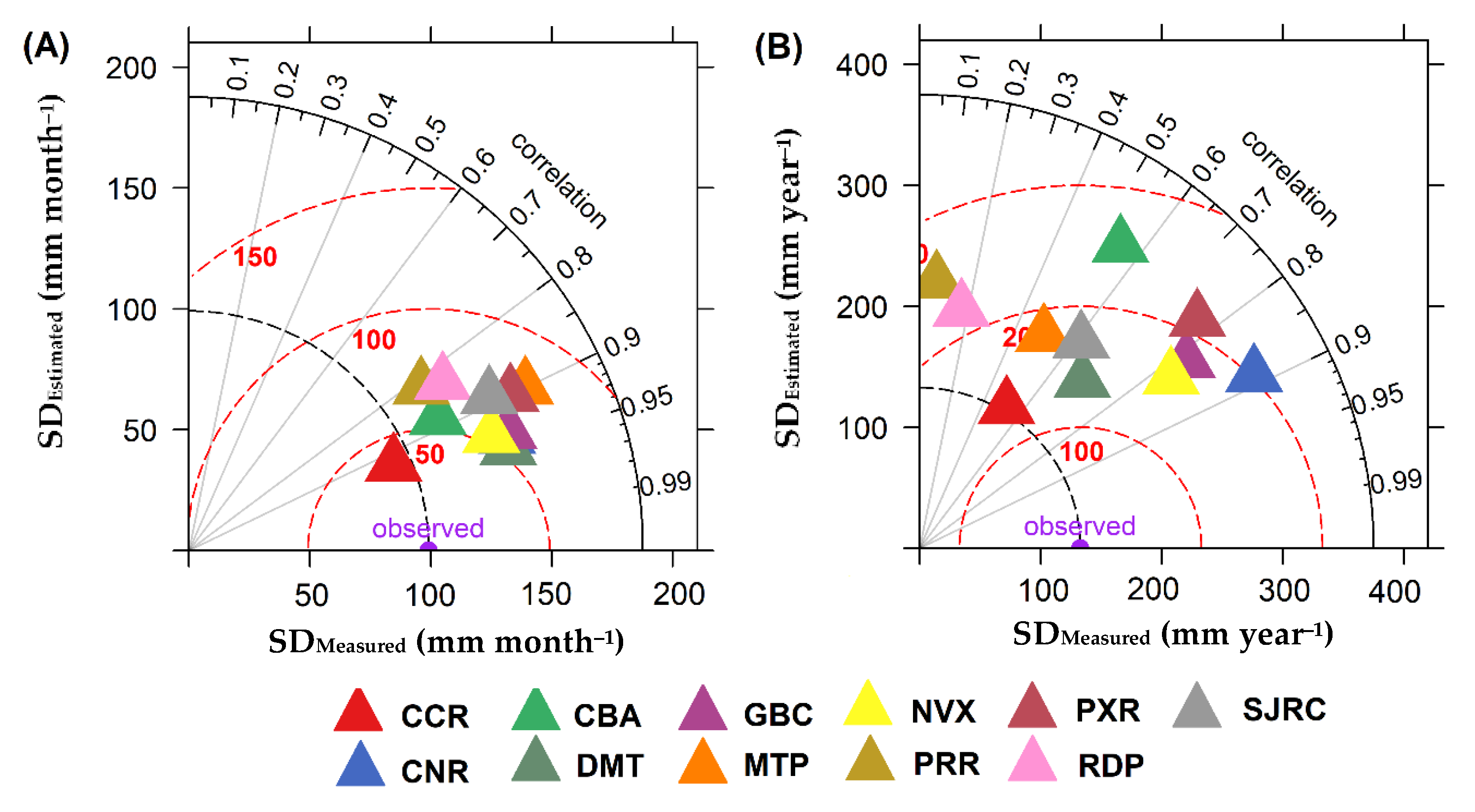
The monthly precipitation estimates by the GPCP had correlation coefficients ranging from 0.81 to 0.95 and Willmott’s coefficients ranging from 0.88 to 0.97. The highest coefficients were obtained in DMT (r = 0.95, d = 0.97). The smallest error in the monthly precipitation estimates was in CCR (RMSE = 39.14 mm month−1) and the largest was in RDP (RMSE = 75.62 mm month−1) (Figure 10A). The lowest correlation and Willmott coefficients and the highest error in annual precipitation was obtained in PRR (r = 0.06; d = 0.41; RMSE = 456.86 mm year−1). The annual precipitation estimates had the highest correlation coefficient in CNR (r = 0.88), the highest Willmott coefficient in GBC (d = 0.88) and the lowest error in CCR (RMSE = 157.76 mm year−1) (Figure 10B).
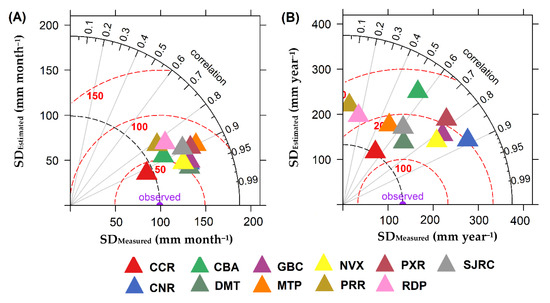
Figure 10.
Taylor diagrams showing the comparisons of (A) monthly (mm month−1) and (B) annual (mm year−1) of the GPCP product at each of the weather stations in the state of Mato Grosso, Brazil. In panels (A,B), the Pearson correlation coefficient (r) was represented by the azimuth angle (black outlines), the RMSE was represented by the red dashed outlines, and the standard deviation (SD) was indicated by the axes x and y, respectively. For (A), the monthly values for the entire study period were averaged, while for (B), the annual values for all years during the study period were averaged.
4. Discussion
Generally, this analysis indicated that remote sensing and reanalysis products performed better in the northern part of the state where the greatest precipitation amounts occur. The identification of a precipitation product with a high accuracy of daily, monthly, or annual estimates varies according to the study site. However, the results showed that products from remote sensing were more accurate than those based on reanalysis [29].
4.1. Assessment of Temporal Accuracy
The daily precipitation estimates by all products had lower performance compared with those at the monthly and annual time scales when assessed against the measurements. This is because remote sensing products are based on instantaneous observations, for example, 3 h intervals (discrete observations) which are then scaled over a given pixel to daily precipitation values, while local measurements provide accumulated/averaged over time (continues observations). Although the products by GLDAS, MERRA, and GPCP do not directly use data from these sensors, they can present these errors, as they indirectly use products based on these sensors in their models. Thus, the longer the precipitation accumulation period, the greater the probability these products will estimate values close to those measured at the surface [30]. Moreover, the rapid development of convective precipitation processes in the region is common. These products are unable to estimate daily precipitation with the same precision as the weather stations [31]. The monthly and annual precipitation estimated by the TRMM and GPM products showed higher correlation and Willmott coefficients and smaller errors. This occurred because the remote sensing precipitation estimates assimilate a higher frequency of high intensity events [32].
4.2. Spatial Variability
In contrast, the spatial differences between precipitation estimates by remote sensing and reanalysis, and the measurements at the weather stations can be partly due to differences in the spatial scales represented by these techniques. A rain gauge consists of a point measurement, while the gridded products (i.e., satellites and land surface models or reanalysis) obtain an average value over the analyzed pixel, although there are different adjustments depending on the local characteristics of each region [33,34]. As a result, satellites and reanalysis products have the ability to estimate precipitation events in areas that a rain gauge was unable to record [30]. It should be noted that remote sensing products can mistakenly estimate precipitation events due to the thickness and temperature of clouds [34].
The GLDAS product uses data from several satellites and rain gauges in its model. The satellite information is based on infrared and microwave sensors, including the TRMM satellite, which justified its relatively improved results [18]. On the other hand, there are some uncertainties that can occur in the data used in developing the GLDAS product, due to the small number of rain gauges and the quality of their measurements in the region [29].
The GPCP tended to overestimate precipitation because the region is strongly influenced by mesoscale convective systems and cold fronts, which provide strong convection and cloud formation (Cirrus), which are more complex to assimilate [35]. As with the GLDAS product, GPCP uncertainties may increase due to the fact that this product uses and combines indirect estimates of precipitation from satellite sensors (visible, infrared, and microwave) as well as rain gauges to calibrate its input data [36].
The MERRA product had noticeable limitations as it underestimated precipitation in all locations, and it percutaneously estimated precipitation events that were not measured at the weather stations [37]. In addition, this reanalysis product has a low spatial resolution—a characteristic that makes it difficult to estimate and detect the occurrence of precipitation events in Mato Grosso where precipitation events have high spatiotemporal variability and are mainly influenced by convective events. Convective precipitation events are more complex to be assimilated by reanalysis models [32,38,39,40].
Moreover, MERRA uses average surface precipitation data (rain gauges) to establish its initial conditions from the National Oceanic and Atmospheric Administration (NOAA) Unified Gauge-Based Analysis of Global Daily Precipitation. Therefore, the estimated precipitation in the center of South America has low accuracy due to the low density of pluviometric stations—indicating an issue of discontinuity in precipitation measurements [20]. There was not enough information available about how many precipitation stations within Mato Grosso were directly used in developing MERRA, if any. The study by [20] indicated that MERRA estimates showed increased error in the Amazon due to sharp decline in the number of precipitation stations used in MERRA from 350 between 1980–2004 to only 65 since 2004. Precipitation estimates by MERRA are closely dependent on the GEOS-5 Catchment land surface model, which can also be highly sensitive to changes in other hydrological variables. In addition, the precipitation measurements used as input in the GEOS-5 model can generate uncertainty in the estimates because the model and the calibration period of the instruments are heterogeneous [40]. A study carried out in the central region of South America, evaluated the MERRA estimates based on an earlier version of this product and found an opposite relationship with the surface precipitation data. The study justified this error due to the low density of installed rain gauges in this region [41].
5. Conclusions
The objective of the study was to compare precipitation estimates based on remote sensing from GPM, TRMM, and GPCP; and reanalysis from GLDAS and MERRA products with measurements from conventional weather stations over the state of Mato Grosso. In general, temporally, both remote sensing and reanalysis precipitation products have satisfactorily estimated the monthly and much of the annual amounts. However, at daily time scales, some of these products showed low correlations with the measurements from. Precipitation estimates by the remote sensing products from GPM, TRMM, and GPCP had better performance compared to those based on reanalysis from GLDAS and MERRA. Precipitation products from GPM have an advantage over those from TRMM and GPCP. The performance of GPM and TRMM products, from high to low, was followed by those from the GPCP and GLDAS while MERRA showed the lowest performance.
Spatially, precipitation estimates by TRMM, GPM, GPCP, and GLDAS showed higher correlation coefficients, from high to low, and lower errors, from low to high, respectively within the Amazon biome in the northern region than in the Cerrado and Pantanal in the southern regions of Mato Grosso. In contrast, MERRA estimates showed lower correlation and higher errors in all regions of the state. These findings, though, should be viewed along with the fact that the northern part of the state is represented by large scale tropical precipitation and cloud systems with less spatial variability that make it easy to estimate precipitation. These systems gradually become small scale scattered and more spatially variable clouds towards the southern regions as the climate eventually transition to subtropical when moving more south. While the northern region was represented with low density measurements stations, the southern regions were represented with relatively higher measurements density but not high enough to capture the spatial variability of these small-scale cloud systems. This combination should explain the performance of these precipitation estimates from north to south of Mato Grosso.
This study demonstrated which remote sensing and reanalysis products can best serve as an alternative in the absence of rain gauge measurements. The findings of this assessment are expected to aid research and applications that require this type of precipitation data in Mato Grosso including sustainable agricultural production, hydrological analysis, water resources management, and drought management. Finally, this study also indicated that it is important to increase the number of weather stations to allow for a more spatially representative evaluation of precipitation estimates and measurement.
Author Contributions
Conceptualization, A.L.P.J., M.S.B., N.G.M., G.L.V. and H.M.E.G.; methodology, A.L.P.J., M.S.B., N.G.M. and C.A.S.Q.; software, A.L.P.J. and M.S.B.; validation, A.L.P.J., M.S.B., N.G.M., L.O.F.d.S., H.M.E.G. and N.L.N.; formal analysis, A.L.P.J., M.S.B., N.G.M., G.L.V., H.M.E.G., I.O.I. and N.L.N.; investigation, A.L.P.J. and M.S.B.; resources, A.L.P.J.; data curation, A.L.P.J. and A.L.P.J.; writing—original draft preparation, A.L.P.J., M.S.B. and N.G.M.; writing—review and editing, M.S.B., N.G.M., G.L.V. and H.M.E.G.; visualization, M.S.B. and H.M.E.G.; supervision, M.S.B.; project administration, M.S.B.; funding acquisition, M.S.B. All authors have read and agreed to the published version of the manuscript.
Funding
This research was partially funded by Conselho Nacional de Desenvolvimento Científico e Tecnológico (CNPq), code #407463/2016-0, #310879/2017-5 and #305761/2018-8, Fundação de Amparo à Pesquisa do Estado de Mato Grosso (FAPEMAT), code #561397/2014, Universidade Federal de Mato Grosso (UFMT), Programa de Pós-Graduação em Física Ambiental (PPGFA/IF/UFMT), Instituto Federal de Mato Grosso (IFMT), the National Science Foundation (NSF) Award Number IIA-1301346, and New Mexico State University.
Institutional Review Board Statement
Not applicable.
Informed Consent Statement
Not applicable.
Data Availability Statement
Publicly available datasets were analyzed in this study. The data can be found here (https://giovanni.gsfc.nasa.gov/giovanni/; http://portal.inmet.gov.br).
Acknowledgments
The authors would like to thank the Giovanni Platform of the National Aeronautics and Space Administration (NASA) and Instituto National de Meteorologia (INMET) to provide data to this research. The authors would like to thank two anonymous reviewers for providing useful reviews that helped in strengthening the manuscript.
Conflicts of Interest
The authors declare no conflict of interest. The funders had no role in the design of the study; in the collection, analyses, or interpretation of data; in the writing of the manuscript, or in the decision to publish the results. Any opinions, findings, and conclusions or recommendations expressed in this material are those of the author(s) and do not necessarily reflect the views of the National Science Foundation.
References
- IBGE | Cidades@ | Mato Grosso | Panorama. Available online: https://cidades.ibge.gov.br/brasil/mt/panorama (accessed on 2 November 2020).
- Machado, N.G.; Santos, G.T.; Biudes, M.S.; Silva, J.L.; Bacarji, A.G.; Costa, M.E.L.; de Bílio, R.S. Sustainable development index of municipalities in Mato Grosso. Rev. Bras. Gestão Desenvolv. Reg. 2020, 16, 222–234. [Google Scholar]
- Gusso, A.; Ducati, J.R.; Bortolotto, V.C. Analysis of Soybean Cropland Expansion in the Southern Brazilian Amazon and Its Relation to Economic Drivers. Acta Amaz. 2017, 47, 281–292. [Google Scholar] [CrossRef]
- Lathuillière, M.J.; Johnson, M.S.; Donner, S.D. Water Use by Terrestrial Ecosystems: Temporal Variability in Rainforest and Agricultural Contributions to Evapotranspiration in Mato Grosso, Brazil. Environ. Res. Lett. 2012, 7, 024024. [Google Scholar] [CrossRef]
- Anderson, M.C.; Zolin, C.A.; Hain, C.R.; Semmens, K.; Yilmaz, M.T.; Gao, F. Comparison of Satellite-Derived LAI and Precipitation Anomalies over Brazil with a Thermal Infrared-Based Evaporative Stress Index for 2003–2013. J. Hydrol. 2015, 526, 287–302. [Google Scholar]
- Da Amorim, J.S.; Viola, M.R.; Junqueira, R.; de Oliveira, V.A.; de Mello, C.R. Evaluation of Satellite Precipitation Products for Hydrological Modeling in the Brazilian Cerrado Biome. Water 2020, 12, 2571. [Google Scholar] [CrossRef]
- Oliveira, P.T.S.; Nearing, M.A.; Moran, M.S.; Goodrich, D.C.; Wendland, E.; Gupta, H.V. Trends in Water Balance Components across the Brazilian Cerrado. Water Resour. Res. 2014, 50, 7100–7114. [Google Scholar] [CrossRef]
- Arvor, D.; Dubreuil, V.; Ronchail, J.; Simões, M.; Funatsu, B.M. Spatial Patterns of Rainfall Regimes Related to Levels of Double Cropping Agriculture Systems in Mato Grosso (Brazil). Int. J. Climatol. 2014, 34, 2622–2633. [Google Scholar]
- Santos, A.B.; Heil Costa, M.; Chartuni Mantovani, E.; Boninsenha, I.; Castro, M. A Remote Sensing Diagnosis of Water Use and Water Stress in a Region with Intense Irrigation Growth in Brazil. Remote Sens. 2020, 12, 3725. [Google Scholar] [CrossRef]
- Arvor, D.; Meirelles, M.; Dubreuil, V.; Begue, A.; Shimabukuro, Y.E. Analyzing the Agricultural Transition in Mato Grosso, Brazil, Using Satellite-Derived Indices. Appl. Geogr. 2012, 32, 702–713. [Google Scholar]
- Machado, N.G.; Biudes, M.S.; Querino, C.A.S.; de Morais Danelichen, V.H.; Velasque, M.C.S. Seasonal and Interannual Pattern of Meteorological Variables in Cuiabá, Mato Grosso State, Brazil. Braz. J. Geophys. 2015, 33, 477–488. [Google Scholar] [CrossRef]
- Biudes, M.S.; Vourlitis, G.L.; Machado, N.G.; de Arruda, P.H.Z.; Neves, G.A.R.; de Almeida Lobo, F.; Neale, C.M.U.; de Souza Nogueira, J. Patterns of Energy Exchange for Tropical Ecosystems across a Climate Gradient in Mato Grosso, Brazil. Agric. For. Meteorol. 2015, 202, 112–124. [Google Scholar] [CrossRef]
- Machado, N.G.; Ventura, T.M.; de Morais Danelichen, V.H.; Querino, C.A.S.; Biudes, M.S. Estimation of Rainfall of Neural Network over a Neotropical Region. Rev. Bras. Climatol. 2015, 17. [Google Scholar] [CrossRef]
- Ferguson, C.R.; Wood, E.F.; Vinukollu, R.K. A Global Intercomparison of Modeled and Observed Land–Atmosphere Coupling. J. Hydrometeorol. 2012, 13, 749–784. [Google Scholar] [CrossRef]
- Khodadoust Siuki, S.; Saghafian, B.; Moazami, S. Comprehensive Evaluation of 3-Hourly TRMM and Half-Hourly GPM-IMERG Satellite Precipitation Products. Int. J. Remote Sens. 2017, 38, 558–571. [Google Scholar] [CrossRef]
- Alvares, C.A.; Stape, J.L.; Sentelhas, P.C.; de Moraes Gonçalves, J.L.; Sparovek, G. Köppen’s Climate Classification Map for Brazil. Meteorol. Z. 2013, 22, 711–728. [Google Scholar] [CrossRef]
- Instituto Nacional de Meteorologia—INMET. Available online: http://portal.inmet.gov.br/ (accessed on 2 November 2020).
- Rodell, M.; Houser, P.R.; Jambor, U.E.A.; Gottschalck, J.; Mitchell, K.; Meng, C.-J.; Arsenault, K.; Cosgrove, B.; Radakovich, J.; Bosilovich, M. The Global Land Data Assimilation System. Bull. Am. Meteorol. Soc. 2004, 85, 381–394. [Google Scholar] [CrossRef]
- Molod, A.; Takacs, L.; Suarez, M.; Bacmeister, J. Development of the GEOS-5 Atmospheric General Circulation Model: Evolution from MERRA to MERRA2. Geosci. Model Dev. 2015, 8, 1339–1356. [Google Scholar] [CrossRef]
- Reichle, R.H.; Liu, Q.; Koster, R.D.; Draper, C.S.; Mahanama, S.P.; Partyka, G.S. Land Surface Precipitation in MERRA-2. J. Clim. 2017, 30, 1643–1664. [Google Scholar] [CrossRef]
- Dinku, T.; Ceccato, P.; Grover-Kopec, E.; Lemma, M.; Connor, S.J.; Ropelewski, C.F. Validation of Satellite Rainfall Products over East Africa’s Complex Topography. Int. J. Remote Sens. 2007, 28, 1503–1526. [Google Scholar] [CrossRef]
- Liu, Z.; Ostrenga, D.; Teng, W.; Kempler, S. Tropical Rainfall Measuring Mission (TRMM) Precipitation Data and Services for Research and Applications. Bull. Am. Meteorol. Soc. 2012, 93, 1317–1325. [Google Scholar]
- GES DISC Dataset: GPM IMERG Final Precipitation L3 1 Day 0.1 Degree x 0.1 Degree V06 (GPM_3IMERGDF 06). Available online: https://disc.gsfc.nasa.gov/datasets/GPM_3IMERGDF_06/summary (accessed on 2 November 2020).
- GES DISC Dataset: GPCP Precipitation Level 3 Monthly 0.5-Degree V3.0 Beta (GPCPMON 3.0). Available online: https://disc.gsfc.nasa.gov/datasets/GPCPMON_3.0/summary (accessed on 2 November 2020).
- Adler, R.F.; Wang, J.-J.; Gu, G.; Huffman, G.J. A Ten-Year Tropical Rainfall Climatology Based on a Composite of TRMM Products. J. Meteorol. Soc. Jpn. Ser. II 2009, 87, 281–293. [Google Scholar] [CrossRef]
- Willmott, C.J.; Ackleson, S.G.; Davis, R.E.; Feddema, J.J.; Klink, K.M.; Legates, D.R.; O’donnell, J.; Rowe, C.M. Statistics for the Evaluation and Comparison of Models. J. Geophys. Res. Ocean. 1985, 90, 8995–9005. [Google Scholar] [CrossRef]
- Wilks, D.S. Statistical Methods in the Atmospheric Sciences; Academic Press: Cambridge, MA, USA, 2011; Volume 100. [Google Scholar]
- Taylor, K.E. Summarizing Multiple Aspects of Model Performance in a Single Diagram. J. Geophys. Res. Atmos. 2001, 106, 7183–7192. [Google Scholar] [CrossRef]
- Qi, W.; Liu, J.; Chen, D. Evaluations and Improvements of GLDAS2. 0 and GLDAS2. 1 Forcing Data’s Applicability for Basin Scale Hydrological Simulations in the Tibetan Plateau. J. Geophys. Res. Atmos. 2018, 123, 13128–13148. [Google Scholar] [CrossRef]
- Danelichen, V.H.M.; Machado, N.G.; Biudes, M.S.; Souza, M.C. TRMM Satellite Performance in Estimated Rainfall over the Midwest Region of Brazil. Rev. Bras. Climatol. 2013, 12. [Google Scholar] [CrossRef]
- Ebert, E.E.; Janowiak, J.E.; Kidd, C. Comparison of Near-Real-Time Precipitation Estimates from Satellite Observations and Numerical Models. Bull. Am. Meteorol. Soc. 2007, 88, 47–64. [Google Scholar] [CrossRef]
- Sun, Q.; Miao, C.; Duan, Q.; Ashouri, H.; Sorooshian, S.; Hsu, K.-L. A Review of Global Precipitation Data Sets: Data Sources, Estimation, and Intercomparisons. Rev. Geophys. 2018, 56, 79–107. [Google Scholar] [CrossRef]
- Meng, J.; Li, L.; Hao, Z.; Wang, J.; Shao, Q. Suitability of TRMM Satellite Rainfall in Driving a Distributed Hydrological Model in the Source Region of Yellow River. J. Hydrol. 2014, 509, 320–332. [Google Scholar] [CrossRef]
- Dos Santos, L.O.F.; Querino, C.A.S.; da Querino, J.K.A.S.; Pedreira Junior, A.L.; de Moura, A.R.M.; Machado, N.G.; Biudes, M.S. Validation of Rainfall Data Estimated by GPM Satellite on Southern Amazon Region. Rev. Ambiente Água 2019, 14. [Google Scholar] [CrossRef]
- Franchito, S.H.; Rao, V.B.; Vasques, A.C.; Santo, C.M.; Conforte, J.C. Validation of TRMM Precipitation Radar Monthly Rainfall Estimates over Brazil. J. Geophys. Res. Atmos. 2009, 114. [Google Scholar] [CrossRef]
- Darand, M.; Khandu, K. Statistical Evaluation of Gridded Precipitation Datasets Using Rain Gauge Observations over Iran. J. Arid Environ. 2020, 178, 104172. [Google Scholar] [CrossRef]
- Gelaro, R.; McCarty, W.; Suárez, M.J.; Todling, R.; Molod, A.; Takacs, L.; Randles, C.A.; Darmenov, A.; Bosilovich, M.G.; Reichle, R. The Modern-Era Retrospective Analysis for Research and Applications, Version 2 (MERRA-2). J. Clim. 2017, 30, 5419–5454. [Google Scholar] [CrossRef] [PubMed]
- Bosilovich, M.G.; Chen, J.; Robertson, F.R.; Adler, R.F. Evaluation of Global Precipitation in Reanalyses. J. Appl. Meteorol. Climatol. 2008, 47, 2279–2299. [Google Scholar] [CrossRef]
- Pfeifroth, U.; Mueller, R.; Ahrens, B. Evaluation of Satellite-Based and Reanalysis Precipitation Data in the Tropical Pacific. J. Appl. Meteor. Climatol. 2013, 52, 634–644. [Google Scholar] [CrossRef]
- Bosilovich, M.G.; Robertson, F.R.; Takacs, L.; Molod, A.; Mocko, D. Atmospheric Water Balance and Variability in the MERRA-2 Reanalysis. J. Clim. 2017, 30, 1177–1196. [Google Scholar] [CrossRef]
- De Quadro, M.F.L.; da Dias, M.A.F.S.; Herdies, D.L.; de Gonçalves, L.G.G. Climatological Analysis of the Precipitation and Umidity Transport on the SACZ Region Using the New Generation of Reanalysis. Rev. Bras. Meteorol. 2012, 27, 152–162. [Google Scholar] [CrossRef]
Publisher’s Note: MDPI stays neutral with regard to jurisdictional claims in published maps and institutional affiliations. |
© 2021 by the authors. Licensee MDPI, Basel, Switzerland. This article is an open access article distributed under the terms and conditions of the Creative Commons Attribution (CC BY) license (http://creativecommons.org/licenses/by/4.0/).


