1. Introduction
Plastic pollution currently represents one of the most important environmental challenges, since it negatively affects ecosystems, aquatic life, and human health. Plastic is an inexpensive, lightweight, malleable, and durable synthetic organic material made from hydrocarbons, whose popularity soared during the 20th century. At present, plastic is often used for single-use purposes and its annual production is predicted to increase by six times between 2015 and 2050 [
1]. Although several research studies assessed plastic pollution in marine environments and raised the awareness of potential damages to oceans, relatively little work has been done on freshwater ecosystems, especially regarding plastic transport dynamics [
2]. Indeed, rivers are important vectors of plastic debris to seas and oceans, and their ecosystems are directly affected by this pollution [
2]. The first attempts in quantifying plastic debris transport in rivers were done in the 2010s, investigating the variations of plastic debris concentrations over space and time. These focused on major river such as the Thames [
3] and the Tamar in the United Kingdom (UK) [
4], the Seine in France [
5], the Austrian Danube [
6], and the Dutch Rhine [
7]. On the other hand, complementary to the river case studies, first predictions of plastic debris emissions into seas and oceans were performed by means of modeling approaches [
8,
9,
10]. These studies represent fundamental contributions since they highlight the geographical distribution of plastic pollution and plastic debris transport.
In order to assess its environmental impact and identify the sources, plastic debris is usually grouped into four main categories according to mean diameter size: nanoplastics, microplastics, mesoplastics, and macroplastics [
11]. Note that, depending on the authors, slightly different classifications can be found in the literature [
12]. It is noteworthy that research studies on freshwater plastic pollution have mainly been limited to the nano- and microplastic fractions [
13], while only few works focused on meso- and macroplastic debris up until the study conducted by [
14]. These previous studies pointed out that the transport and the input of plastic debris in riverine environments are controlled by both natural (e.g., hydrodynamics and morphology) and anthropogenic (e.g., plastic waste production and management) characteristics of the catchments [
15,
16,
17]. Furthermore, the main portion of freshwater plastic debris is represented by macroplastics [
18]. Therefore, it becomes crucial to focus on plastic transport dynamics in order to efficiently tackle water plastic pollution issues. Since its storage and remobilization cycle may last for centuries, it is also important to account for long preservation times [
19]. In addition, the recent pandemic originated by the severe acute respiratory syndrome coronavirus 2 (i.e., SARS-CoV-2) led to a dramatic increase in single-use personal protective equipment (PPE) waste, such as disposable face masks made of nonwoven fabrics and latex/plastic gloves [
20]. As a consequence of governmental policies to contain the spread of the virus, an enormous amount of medical waste was produced, mainly composed of plastic-based single-use PPE [
21]; as an example, Spain and China registered medical waste increments of 350% and 370%, respectively [
22]. Although the surface water quality improved during the lockdown due to the closing down of many industries and anthropogenic activities [
23,
24], the macroplastic pollution in freshwater environments has dramatically increased in the last year. It is worth remarking that masks are made of polypropylene (PP) and polyethylene terephthalate (PET) and gloves are made of nonwoven materials and latex [
25,
26,
27]. In addition, [
28] reported that most of the microplastic microfibers in the Magdalena River, Columbia, originates from the degradation of nonwoven synthetic textiles. Thus, it is reasonable to assume that such items are contributing and will contribute to an increase in the plastic pollution of rivers and oceans.
Some countermeasures were recently developed to intercept plastic elements in rivers. Among others, the nonprofit organization Ocean Cleanup developed a new technology to control plastic transport in rivers [
29]. Specifically, they built The Interceptor™, a system that can stop and collect plastic elements in rivers. This system is made of a floating barrier conveying plastic to a solar-powered robot (the Interceptor). In principle, this system can be located in any river and is a suitable solution for limiting plastic transport to the sea. Another solution is represented by the so-called bubble barriers [
30]. A bubble screen is originated from a holed tube located diagonally on the bottom of the river/channel. Air bubbles bring plastic elements to the water surface and then to a catchment system at the river side.
However, according to [
2], “additional hydrometeorological and hydraulic data are crucial” in order to enhance the understanding of such a complex phenomenon. Therefore, following the success of the mentioned countermeasures and considering the gap of knowledge pointed out by [
2], our study aims at investigating the influence of the kinematic flow field on the superficial plastic transport, originated from the degradation of PPE and other plastic materials. To this end, a dedicated model was built, and specific laboratory tests were conducted using both isolated structures and structures located in series. The kinematics of the flow field was analyzed under different hydraulic conditions, which were consistent with mean annual flow conditions occurring in different water bodies in Tuscany (Italy). Laboratory tests showed that the efficiency of isolated structures in limiting the downstream transport of plastic elements slightly depends on the angle of inclination of the structure with respect to the channel wall and on different materials, in the tested range of parameters. Conversely, the efficiency is affected by the average velocity of the approaching flow (i.e., by the approaching Froude number of the flow) and increases in the case of structures disposed in series. Although field data are necessary to validate laboratory results and investigate potential scale effects, this analysis provides some unprecedented and interesting results on the influence of in situ flow conditions on superficial plastic transport in the presence of intercepting barriers.
2. Materials and Methods
An experimental campaign was undertaken in the hydraulics laboratory of the University of Pisa using various kinds of trapping structures. The experiments were carried out in a straight channel having the following characteristics: length = 7.6 m, width (
B) = 0.6 m, and height = 0.5 m. Primarily, two different kinds of structures were tested, i.e., full-width structures (ranging across the entire width of the channel) and partial structures (ranging across partial width of the channel). The full-width structures used in the study were termed
S1,
S2,
S3, and
S4 and are shown in
Figure 1a–d, respectively. Likewise, the partial structures employed in this study are illustrated in
Figure 2. For all the tested configurations, the depth of the submerged part of the structure was approximately equal to 3 mm.
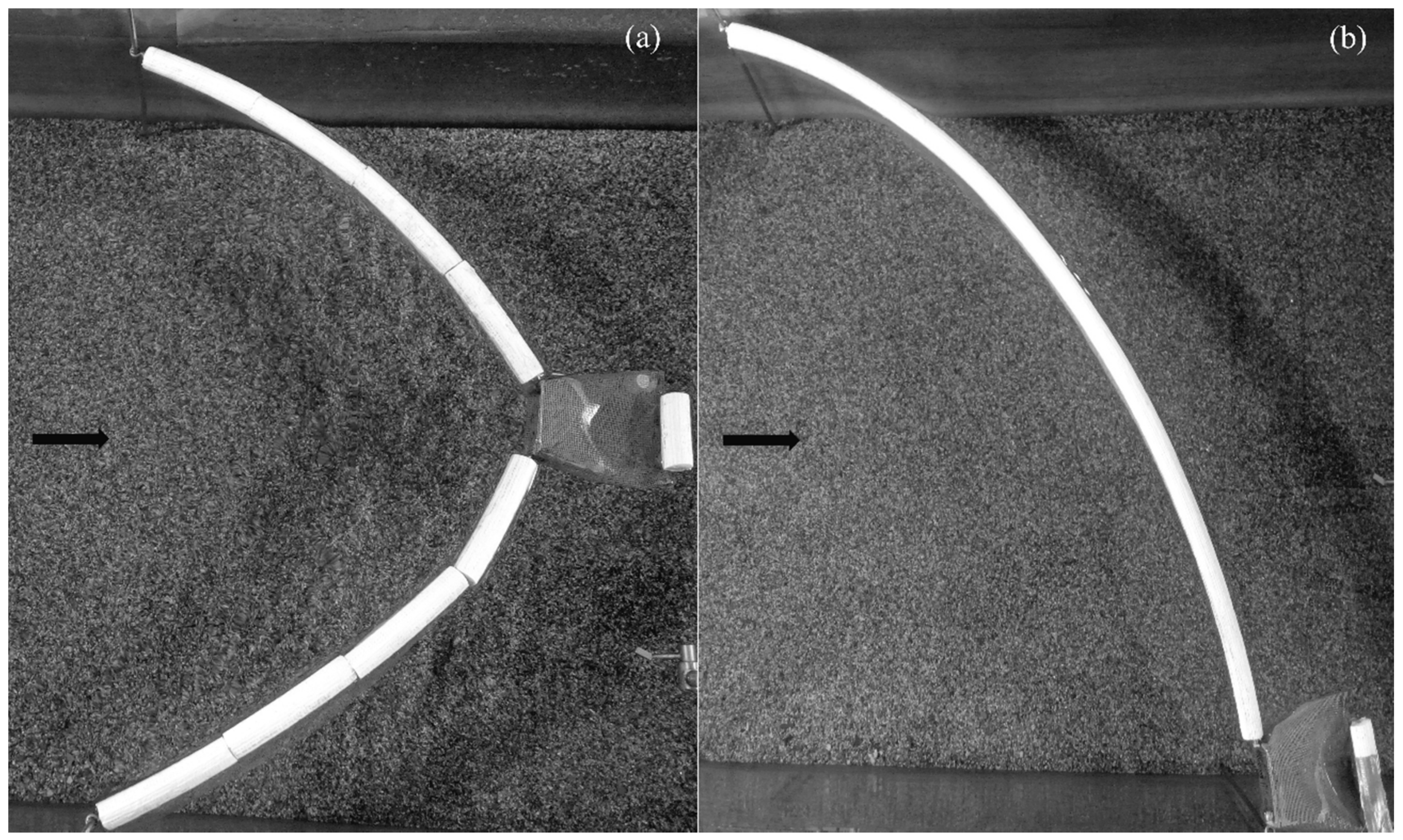
Figure 1a shows the plan view of
S1 which was characterized by two symmetric arms and a trap region located centrally in the channel to accumulate the material flowing in the river. The trap region consisted of a steel mesh box having a square mouth section whose dimensions were 0.05 m × 0.05 m to facilitate the accumulation of floating debris. In
Figure 1a,
lh/
B = 0.48, where
lh is the longitudinal projection of a single arm of the structure. The curved length of one arm of the structure is denoted by
lc and
lc/
B = 0.66. The angle made by the tangent to the arm of the structure with the transversal direction is defined as
α. In this case, α = 45°. The flow discharge is denoted by
Q. The nondimensional longitudinal projection of the trap region (
lt) is defined as
lt/
B = 0.16. The configuration of the trap was identical for all the tested structures.
Figure 1b shows the structure configuration of
S2, which was also symmetric. However, in this case, the lengths of the arms of the structure were shorter and characterized by
lh/
B = 0.21,
lc/
B = 0.5, and α = 25°.
Figure 1c,d correspond to structure configurations
S3 and
S4, respectively, which were asymmetric. These structures were made of a single curved arm ranging across the entire width of the structure, and the trap region was in the vicinity of the channel bank. In this case,
lc represents the curved length of the entire arm. The structure configuration
S3 was characterized by
lh/
B = 0.88,
lc/
B = 1.33, and α = 45°, whereas the parameters for configuration
S4 were
lh/
B = 1.6,
lc/
B = 1.95, and α = 60°.
The partial structures used in this study are shown in
Figure 2.
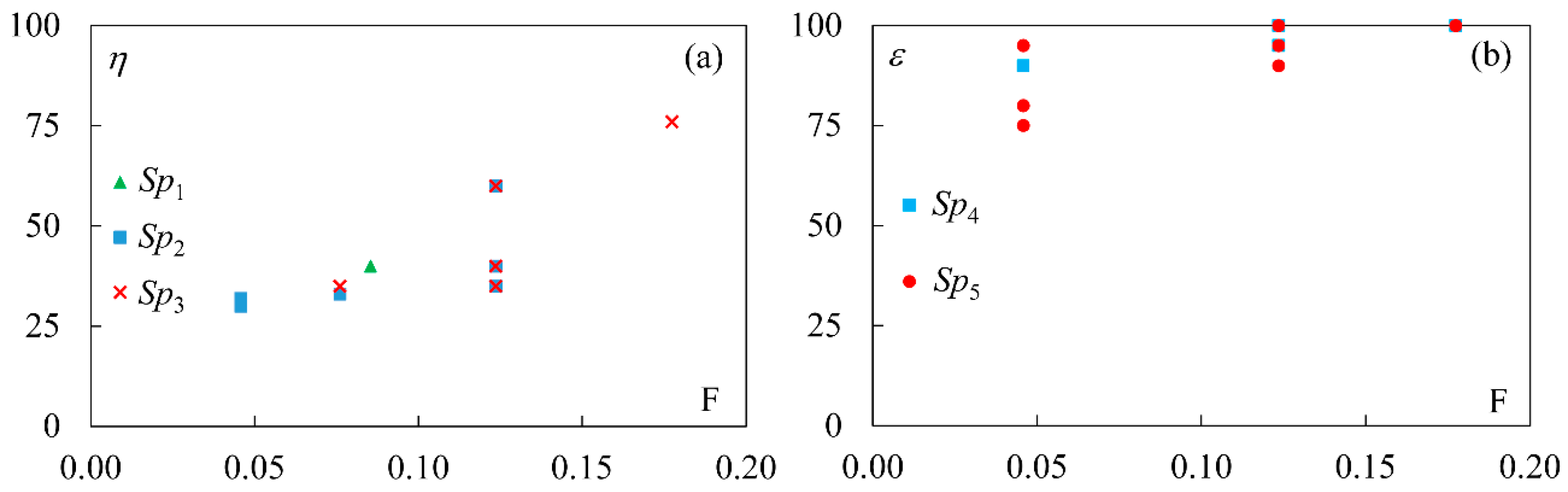
Sp1 was an asymmetric structure covering the partial width of the tested channel (
Figure 2a). In this case, the trap region was located in the vicinity of the channel bank. This structure configuration was characterized by
lh/
B = 0.53,
lv/
B = 0.5,
lc/
B = 0.66, and α = 45°, with
lv indicating the length of projection of the structure including the mouth section in the transversal direction of flow.
Figure 2b shows the structure configuration
Sp2, which was characterized by
lh/
B = 0.4,
lv/
B = 0.65,
lc/
B = 0.66, and α = 30°. Similarly,
Figure 2c shows the structure configuration
Sp3 (
lh/
B = 0.23,
lv/
B = 0.73,
lc/
B = 0.66, and α = 15°). In configuration
Sp4, two
Sp2 structures were used in combination separated by
ld/
B = 1.26, where
ld is the longitudinal distance between the structures in a series arrangement (
Figure 2d). Notably, the trap regions of the two structures in combination were in the vicinity of the opposite banks of the channel. The second structure
Sp2 was characterized by a longer arm length (
lh/
B = 0.53,
lv/
B = 0.8,
lc/
B = 0.91, and α = 30°). Likewise, structure configuration
Sp5 was also tested. This configuration was characterized by a combination of
Sp3 and
Sp2 structures (
Figure 2e), where the second structure with
Sp2 configuration had the same characteristics as that in the structure
Sp4. Pictures of the experimental setups for structure configurations
S1 and
S3 are shown in
Figure 3a,b, respectively.
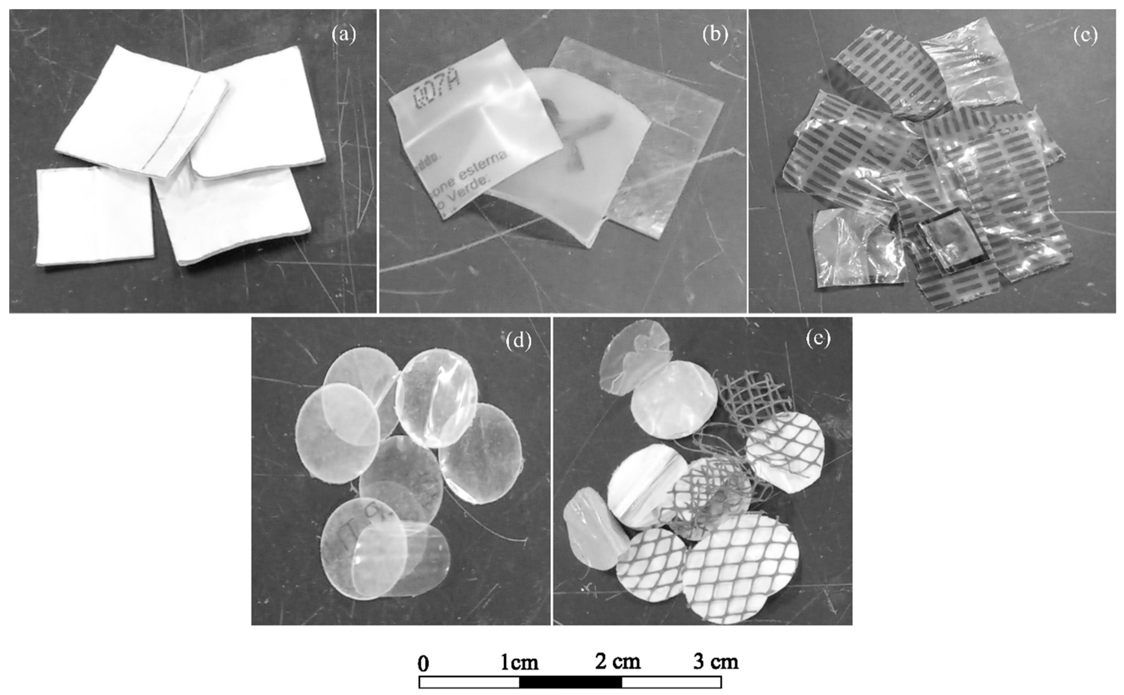
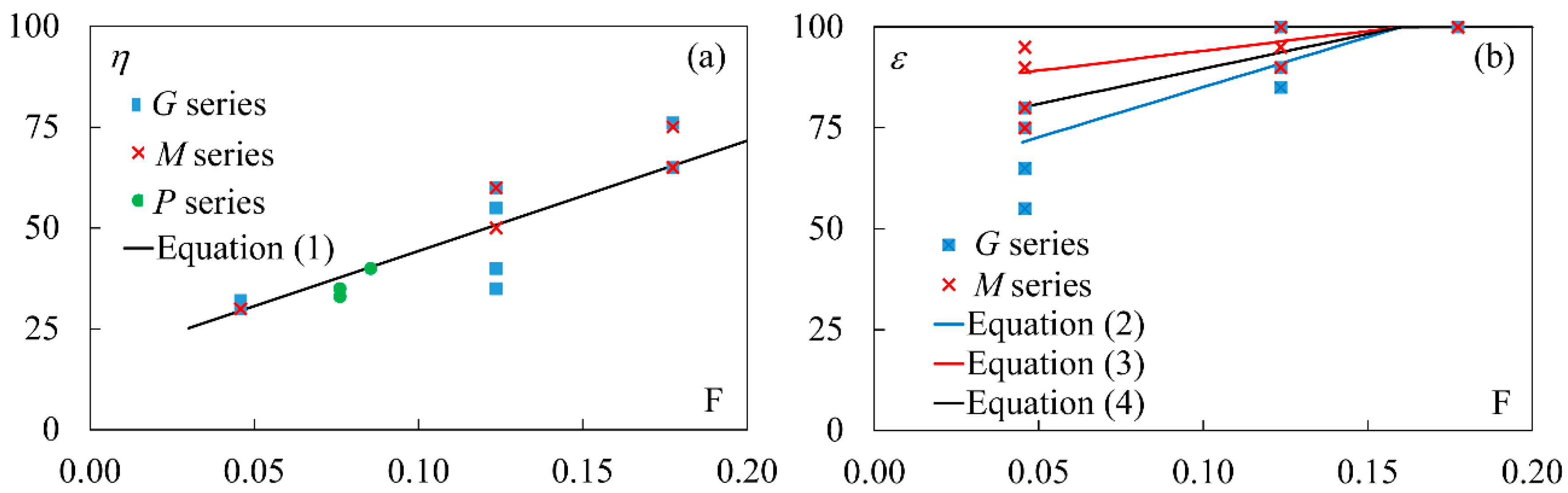
The flow characteristics for experimental tests conducted with different structure configurations and in the presence of three main series of plastic and nonwoven fabric materials were measured (using a Nortek acoustic doppler velocimeter (ADV)) and analyzed. The first series consisted of five types of plastic materials that can be commonly found in rivers (originating from bottles, bags, etc.). They were termed as
P1,
P2,
P3,
P4, and
P5 (
P series) and are shown in
Figure 4a–e, respectively. The
P series had an overall density lesser than 1000 kg/m
3, i.e., lesser than the water density. The individual plastic elements were either square (1.5 cm × 1.5 cm) or circular (
D = 1 cm) in shape, where
D is the diameter of the plastic element. They were tested in conjugation with structure typologies
S1,
S2,
S3,
S4,
Sp1,
Sp2, and
Sp3.
Then plastic and nonwoven fabric elements originating from different components of PPE were also tested, particularly masks and gloves. During the pandemic, huge amounts of PPE waste have been generated, representing another potential source of pollution of water bodies. Therefore, plastic from 10 different types of gloves was tested in this study and termed as
G1,
G2,
G3,
G4,
G5,
G6,
G7,
G8,
G9, and
G10 (
G series). Lastly, nonwoven fabric materials from seven different types of face masks were tested and denoted by
M1,
M2,
M3,
M4,
M5,
M6, and
M7 (
M series). All the above material types are shown in
Figure 5. Like the
P series, the densities of the materials belonging to the
G and
M series were less than 1000 kg/m
3. For test purposes, the materials for
G and
M series were cut into square pieces (1.5 cm × 1.5 cm). Thereafter, they were tested in conjugation with structure configurations
Sp2,
Sp3,
Sp4, and
Sp5. The transport of floating material in the channel due to different hydraulic conditions was tested by varying the tailwater and discharge.
Table 1 reports the hydraulic conditions, as well as the types of structures and materials used in the different tests, with
Q indicating the discharge,
htw indicating the water level, and
vm indicating the average flow velocity in the channel. It is worth noting that the tested range of Froude numbers is consistent with that of some water bodies (e.g., Fiume Morto) in the city of Pisa (Pisa, Italy). Thus, the experimental results of this study can represent a valid aid for future, practical applications.
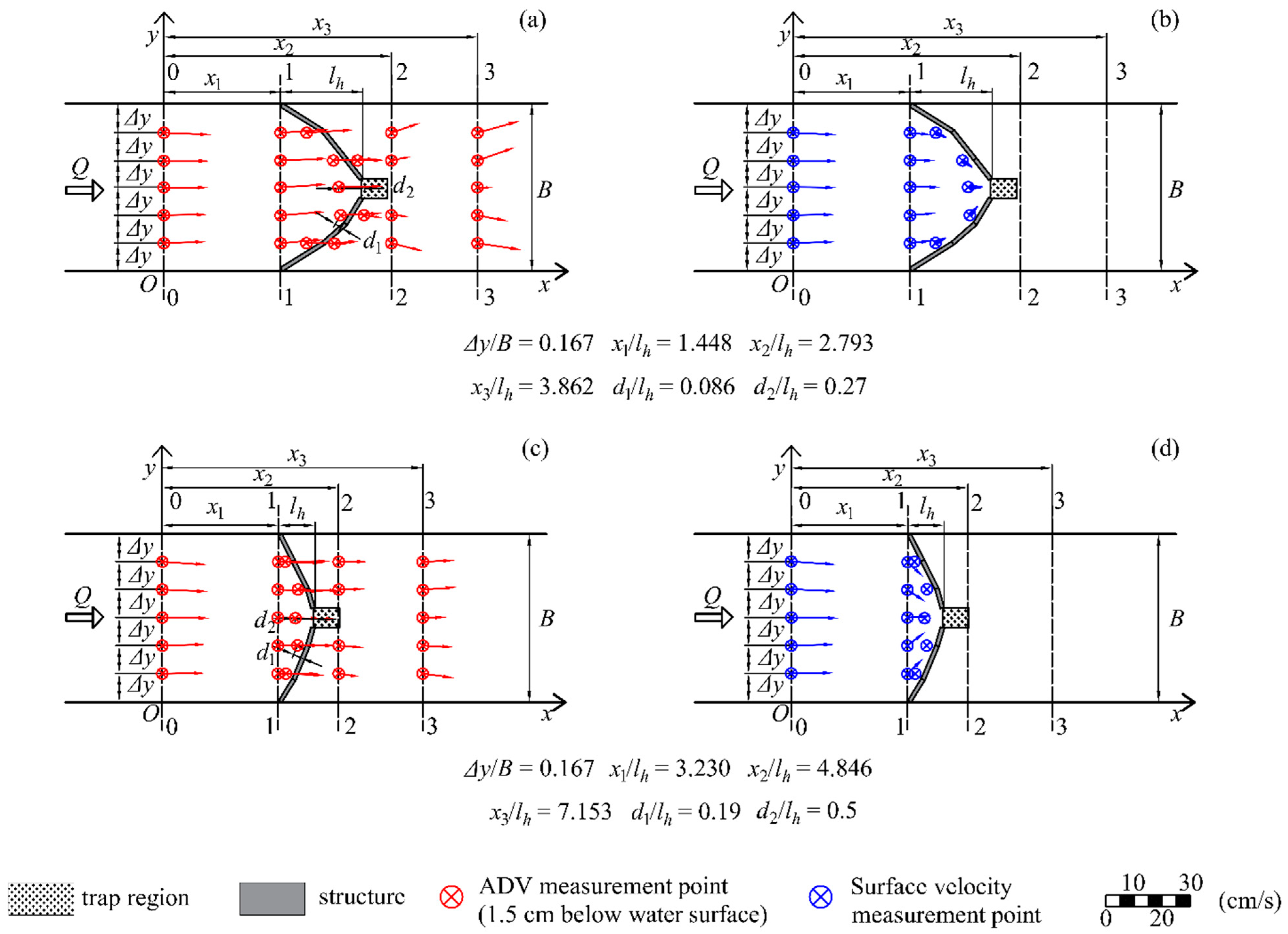
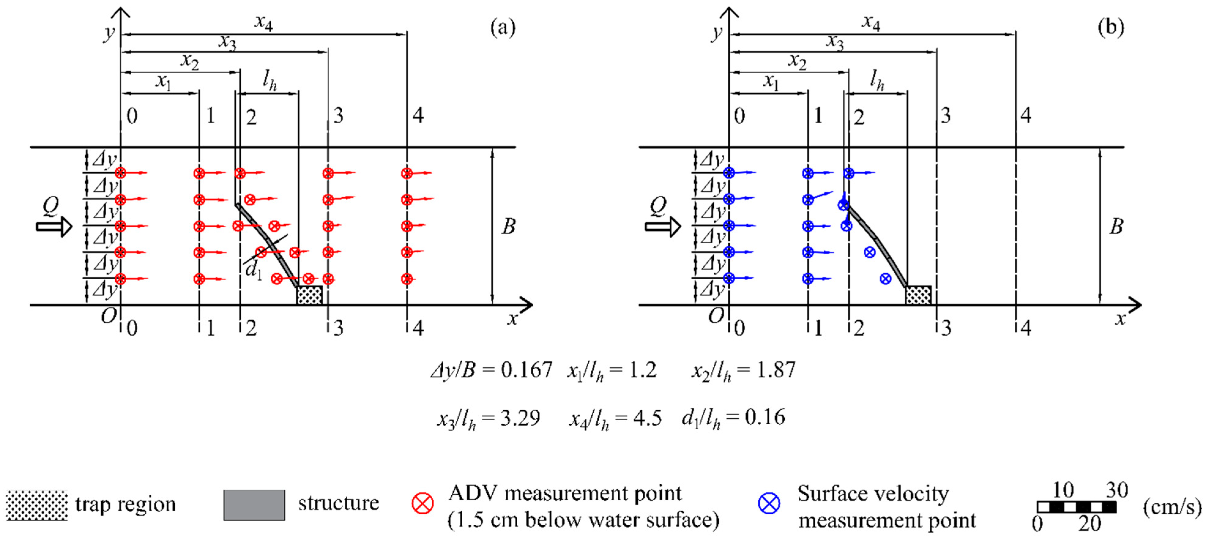
Tests were conducted as follows: primarily, the mobile channel bed was leveled, and water was allowed to enter and reach a desired height. Thereafter, a target discharge
Q was set up, and the water level
htw was made constant using a sluice gate located at the end of the channel. Then, water level measurements were carried out at selected transversal sections both upstream and downstream of the structure, denoted as 0–0, 1–1, 2–2, and 3–3 (see
Figure 6). In each section, measurements were taken at equidistant intervals (Δ
y = 10 cm) in the transversal direction across the entire channel width. Additional measurements were taken along the upstream and downstream contours of the structure, usually around 2.5 cm from the structure (see
Figure 6). Following this, in the case of structure configurations
S1,
S2,
S3,
S4, and
Sp2, the measurements of flow velocities were taken using a Nortek acoustic doppler velocimeter (ADV) at the selected points at
z = 1.5 cm, with
z indicating the depth of the point of measurement from the water surface.
Generally, 15 plastic elements belonging to the
P series were simultaneously released on the water surface 1 m upstream of the structure at equidistant spatial intervals in the transversal direction of the flow across the entire channel width. Their flow pattern was recorded by a high-resolution camera installed above the flume. Their mean velocity at the water surface was estimated from videos and with the help of two measuring tapes attached to both sides of the channel. More specifically, the time taken by macroplastic elements to run across a fixed length was measured in correspondence with the same points upstream of the structure where ADV measurements were taken. This procedure allowed us to estimate the surface velocity magnitude and direction at the selected points. The submerged part of the structure slightly affected measurements taken with the ADV at
z = 1.5 cm. Conversely, the surface velocities resulted to be greatly affected by the presence of the structure. Moreover, for each experiment, the percentage of plastic trapped/stopped by the structure was also noted. This allowed obtaining an estimation of the plastic removal efficiency of each structure, as clarified in a later section. A few special tests were also conducted by mixing plastic elements pertaining to different types of
P series. Results were found to be consistent with those obtained with plastic elements belonging to single types. Successively, the same methodology was adopted for tests conducted with elements belonging to
G and
M series. However, as these tests were essentially conducted using the same range of parameters, ADV measurements were not repeated. However, the analysis of videos also allowed us to estimate the efficiency of the structures in trapping/stopping the floating material.
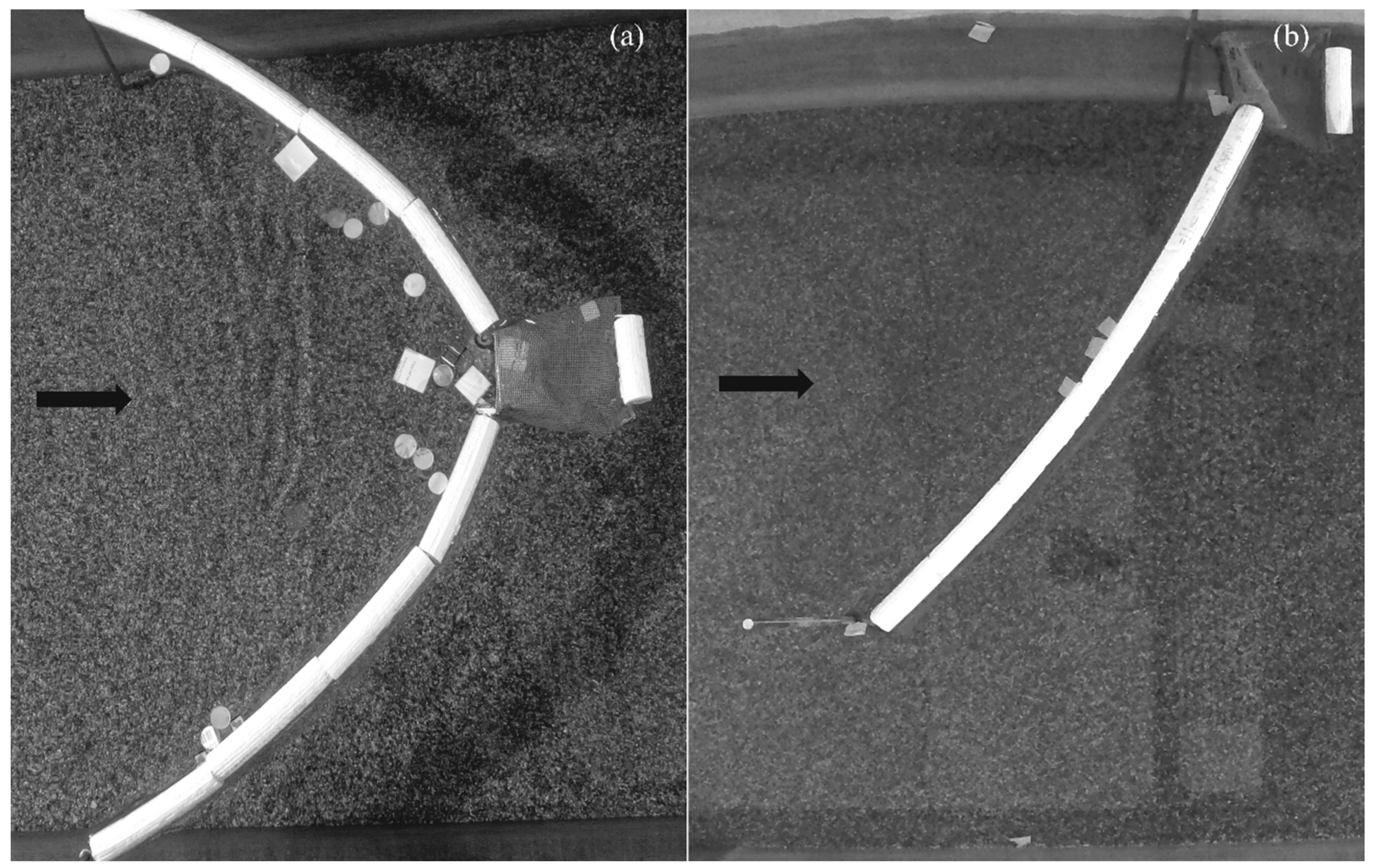
Figure 7a shows a picture of a test conducted with structure configuration
S1 and mixed plastic elements belonging to
P series.
Figure 7b shows the same for a test with structure configuration
Sp2 and plastic type
G6.


