3.1. Case Study I: Measurement of Changes in Bed Morphology
In case study I, the SfM technique was applied to record changes in bed morphology during a physical model study. The objective of the model study was to simulate evolution of river bed morphology during high sediment transport event and to create a database to validate a 1D numerical model developed for simulating river morphology in sediment laden rivers. The study was conducted on a physical hydraulic model representing 1 km long reach of Trishuli River in Nepal (
Figure 1). Trishuli River is a typical Himalayan river with steep bed gradient which becomes relatively flatter after it crosses Betrawati. The selected river reach has an average bed slope of about 1:200 and consists of a sharp bend. The particular reach was chosen for the study since evolvement of river bed morphology is prominent in reaches with flatter bed gradient and with bends.
The 12.5 m long undistorted Froude scaled model at hydraulic laboratory of Hydro Lab in Nepal, representing the 1 km long reach of Trishuli river under study, was built in 1:80 scale. The modelled river channel had a fixed bed which was then filled with sand to provide a mobile bed having an average longitudinal slope of 1:200, in order to match the original bed slope in the prototype. The sand used for preparing mobile bed had median particle diameter (
d50) of 0.55 mm,
d90 of 1.28 mm and geometric standard deviation (
σg) in particle size of 1.972. Similar sediment was also fed with inlet discharge during the simulation. It is to be noted that
d50 of the prototype sediment is about 0.1 mm which shall be represented by model sediment with
d50 = 1.25 microns to fulfill the scaling requirements for an undistorted Froude model. But using such a fine sediment in the model will introduce cohesion in the sediment particles and there is possibility of alteration of sediment transport phenomena from bed load in the prototype to suspended load in the model [
51]. According to Bretschneider, the particle size of sand in models should be greater than 0.5 mm [
52] to avoid the scale effects due to cohesion between sediment particles and changes in flow-grain interaction characteristics. Therefore, a model sediment having
d50 = 0.55 mm was used in this study. A steady discharge of 40 L/s (2290 m
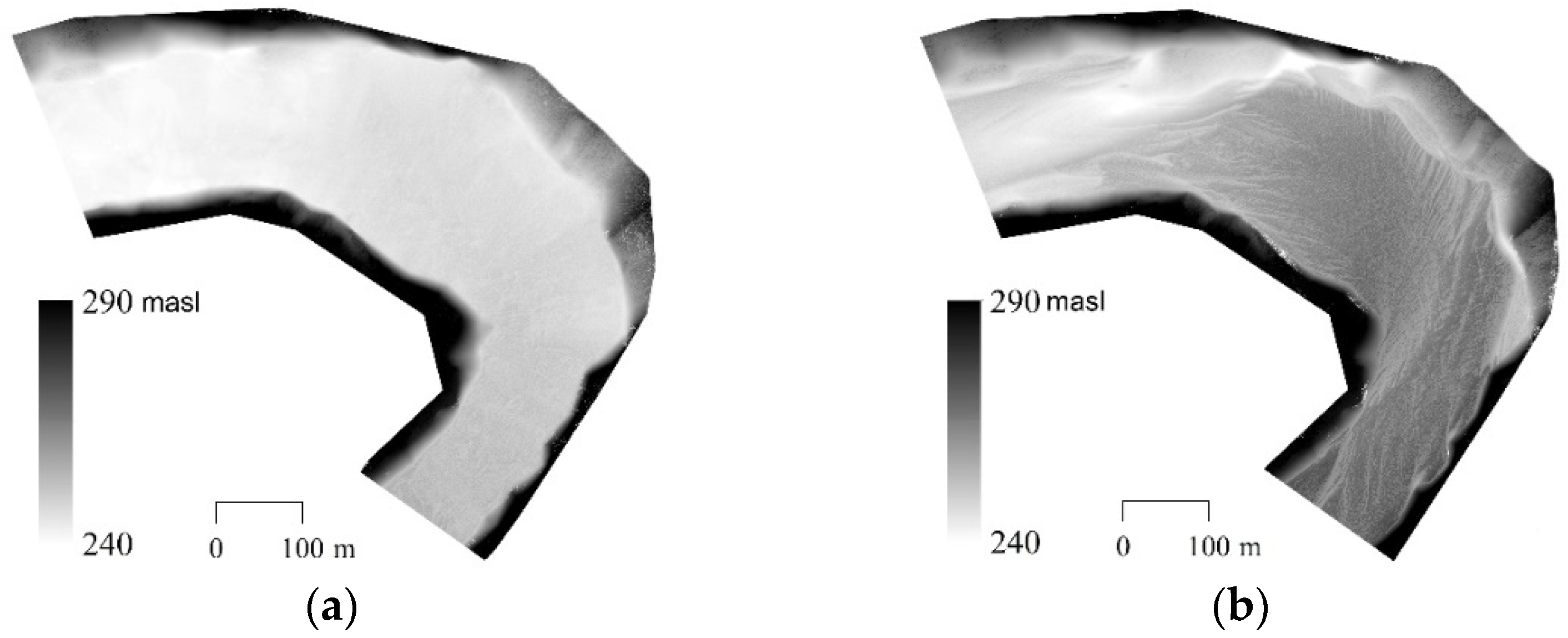
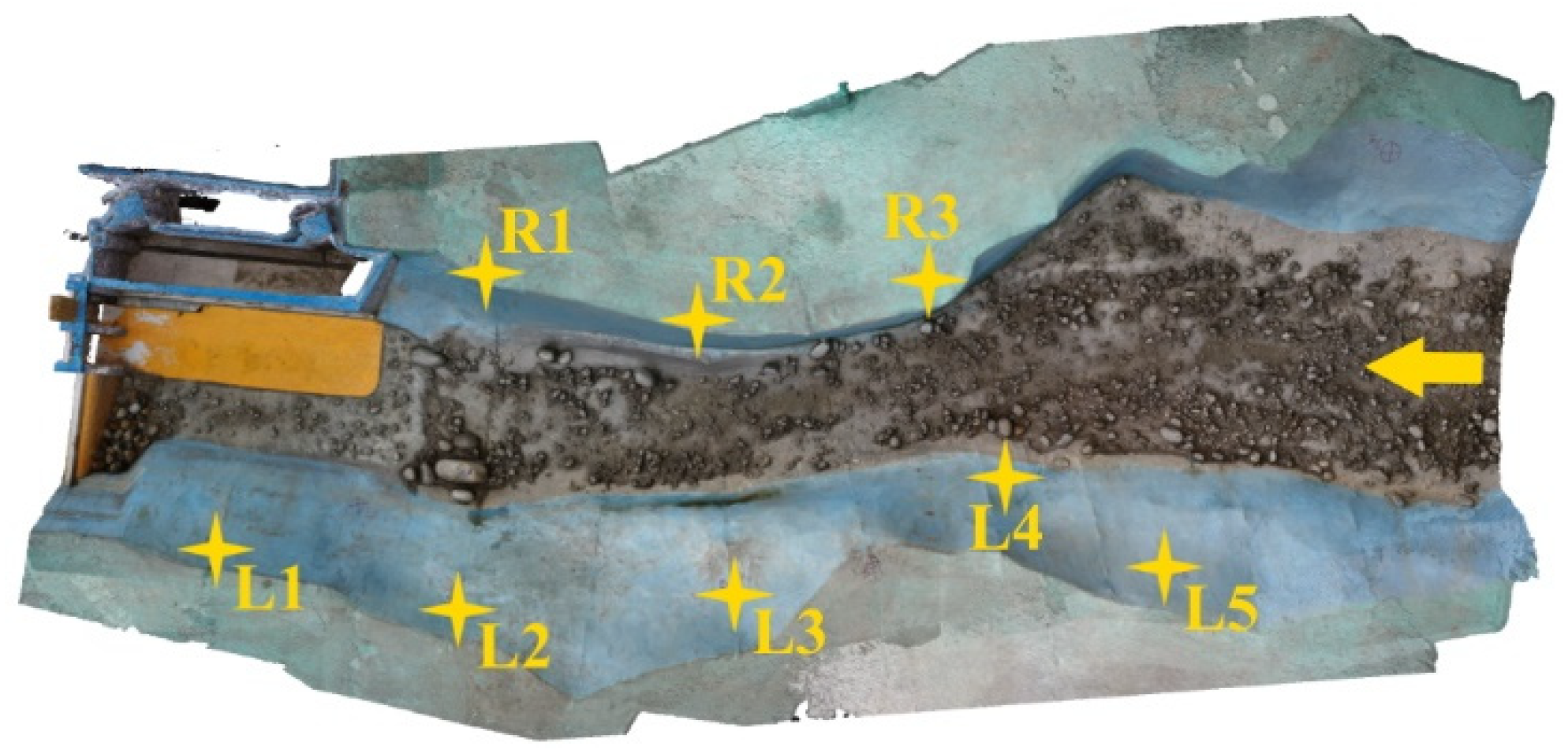
3/s in prototype, which is close to the magnitude of 2 years return period flood) was supplied into the model with sediment feeding at the rate of 10 kg/min which corresponds to sediment concentration of 4167 ppm in the flow. The concentration of sediment fed into the model is about 5 times of average concentration for given discharge as estimated from the site measurement data. The experiment was run for 140 min (about 21 h in prototype) only. Due to high sediment concentration and the flatter river bed gradient, most of the sediment fed with inflow discharge deposited along the channel. The effect of the river bend was clearly visible with the flow concentrating towards the outer bank (the right bank) accompanied with small scour on the initially filled sediment bed while most of the sediment fed was deposited along inner bank (the left bank). A distinct delta front was witnessed propagating to downstream direction, which can be seen in
Figure 2.
The river-bed topographies of initial bed and final river bed after simulation were recorded and respective 3D dense point clouds and DEMs were produced in prototype scale with actual coordinates (meters) and elevations (in masl) using SfM technique. The quality and size of the output dense point clouds and total processing time for each stage were given in
Table 1.
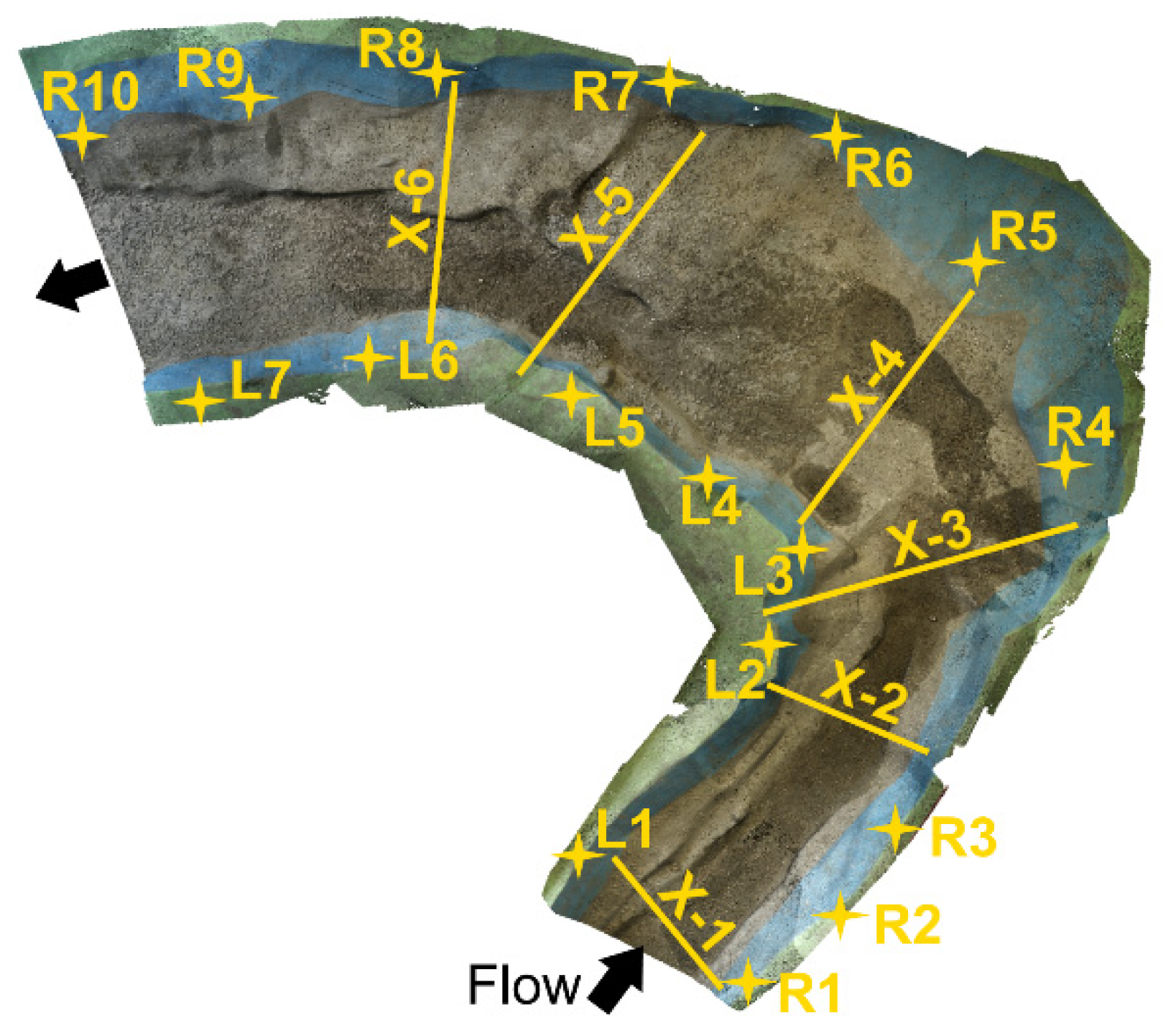
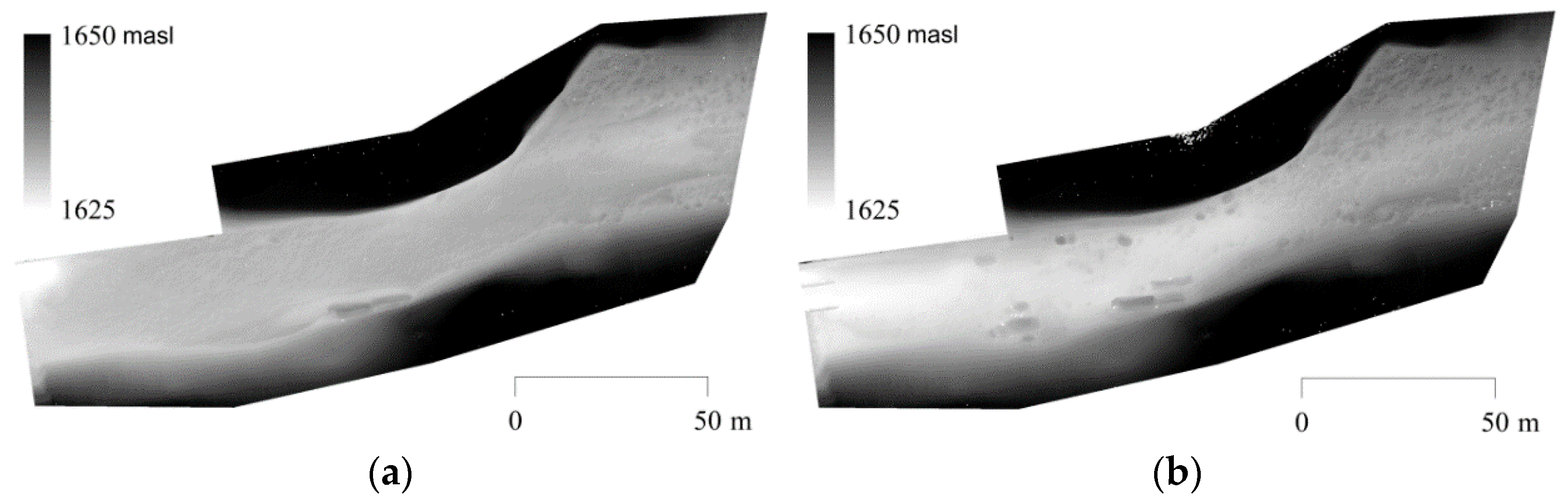
The DEMs of initial river bed and the river bed after test run are shown in
Figure 2a,b respectively. Total 17 GCPs, 10 in the right bank (R1-R10) and 7 in the left bank (L1-L7), distributed over the study area (
Figure 1) were used for georeferencing the 3D models into actual coordinates.
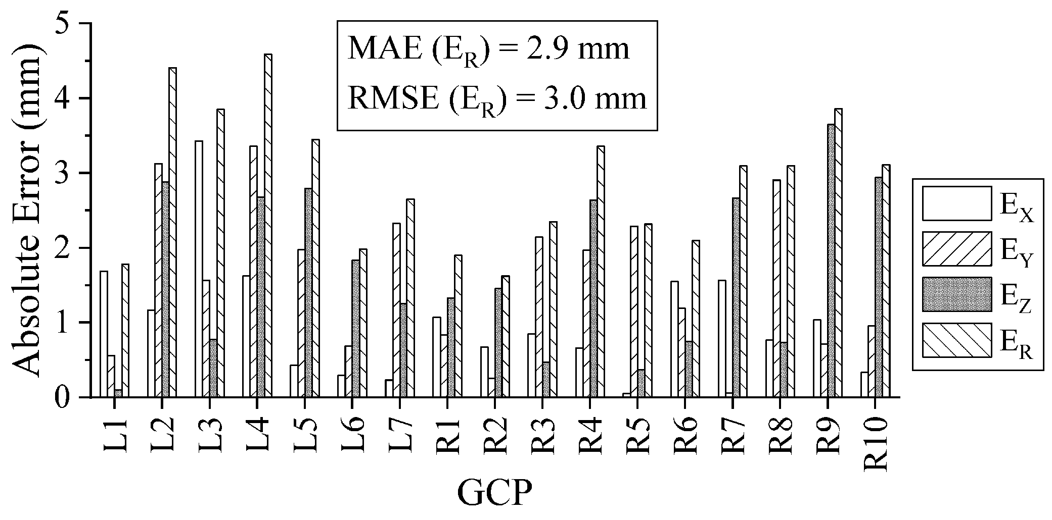
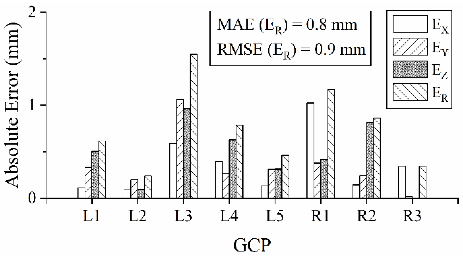
The accuracy of these 3D models was investigated by estimating errors in reproducing 3D location of points, horizontal lengths and cross sections in reference to manual measurements.
Figure 3 shows errors in X, Y and Z coordinates of the selected 17 GCPs in the 3D model, designated as E
x, E
y and E
z respectively. The locations of these points were reproduced in the 3D model with maximum deviation below 4 mm in each direction and the maximum resultant error (E
R) was below 5 mm. Likewise, 12 distances between random pairs of these GCPs were estimated from the 3D model and compared with respective manually measured distances (
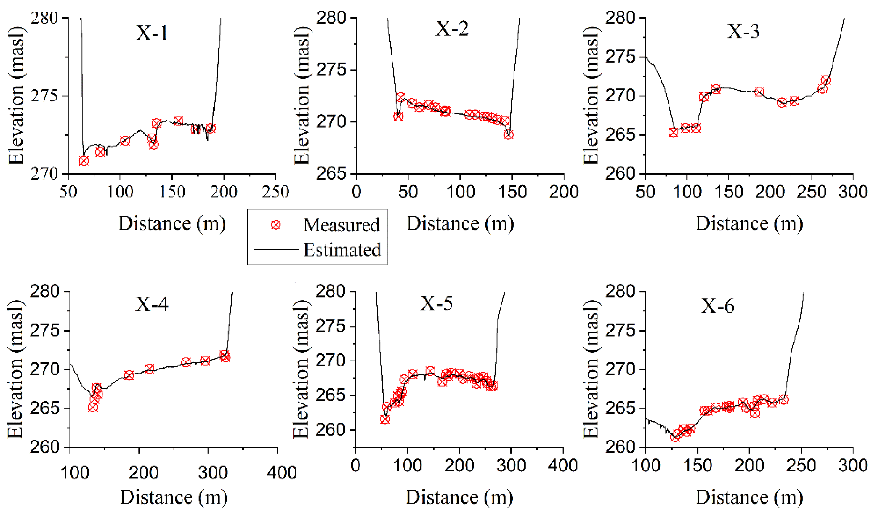
Table 2). The estimated lengths matched pretty well against respective measured distances with root mean square error (RMSE) of 1.9 mm and mean absolute error (MAE) of 1.7 mm. Moreover, 6 cross sections designated as X-1 to X-6 (
Figure 1) were randomly selected over the study area and their cross-section profiles were extracted from the 3D model output for ‘After run scenario’. These estimated cross sections were compared with their respective upscaled cross-section data from manual measurements in the model (
Figure 4), which showed that the estimated cross sections were close to the measured cross sections and had more detailing with abundant points.
After confirming the accuracy of DEMs produced by SfM technique to be within acceptable limits, changes in volume of river bed morphology were calculated using the DEMs generated for initial bed and after run scenarios mentioned above. At the rate of 10 kg/min for 140 min, total 1400 kg sediment was fed with the inflow discharge during the test. Using bulk density of the sediment to be 1680 m3/s, the total volume of sediment added into the system during the test was calculated to be 0.833 m3. Analysing the difference between DEMs for initial bed and river bed after simulation, it showed that 0.677 m3 (out of 0.833 m3 sediment fed into the system) sediment was deposited into whereas 0.125 m3 sediment from initially filled bed was scoured out of the system; which means total 0.281 m3 of sand was transported to downstream of the modelled river reach. To check the accuracy in estimating changes in volume, the volume of sediment trapped at the outlet tank downstream of the model was measured manually using a calibrated bucket. The measured and estimated volumes in model scale were 0.292 m3 and 0.281 m3 respectively with a discrepancy of 4% only.
After the satisfactory result from the test, SfM technique was further applied in full-fledged model study in which intermediate river bed formations at different time steps during the test were also recorded in addition to the initial and final river bed. Besides measuring the changes in bed morphology precisely, SfM technique also made it possible to record the evolution of bed morphology over time by capturing the river bed at different time steps during the test. Moreover, it provided high resolution river bed data for creating mesh of initial river bed to be used in numerical modelling. It also provided high-resolution river bed data for intermediate time steps for validating the results from the numerical model.
3.2. Case Study II: Evaluation of Sediment Flushing Efficiency
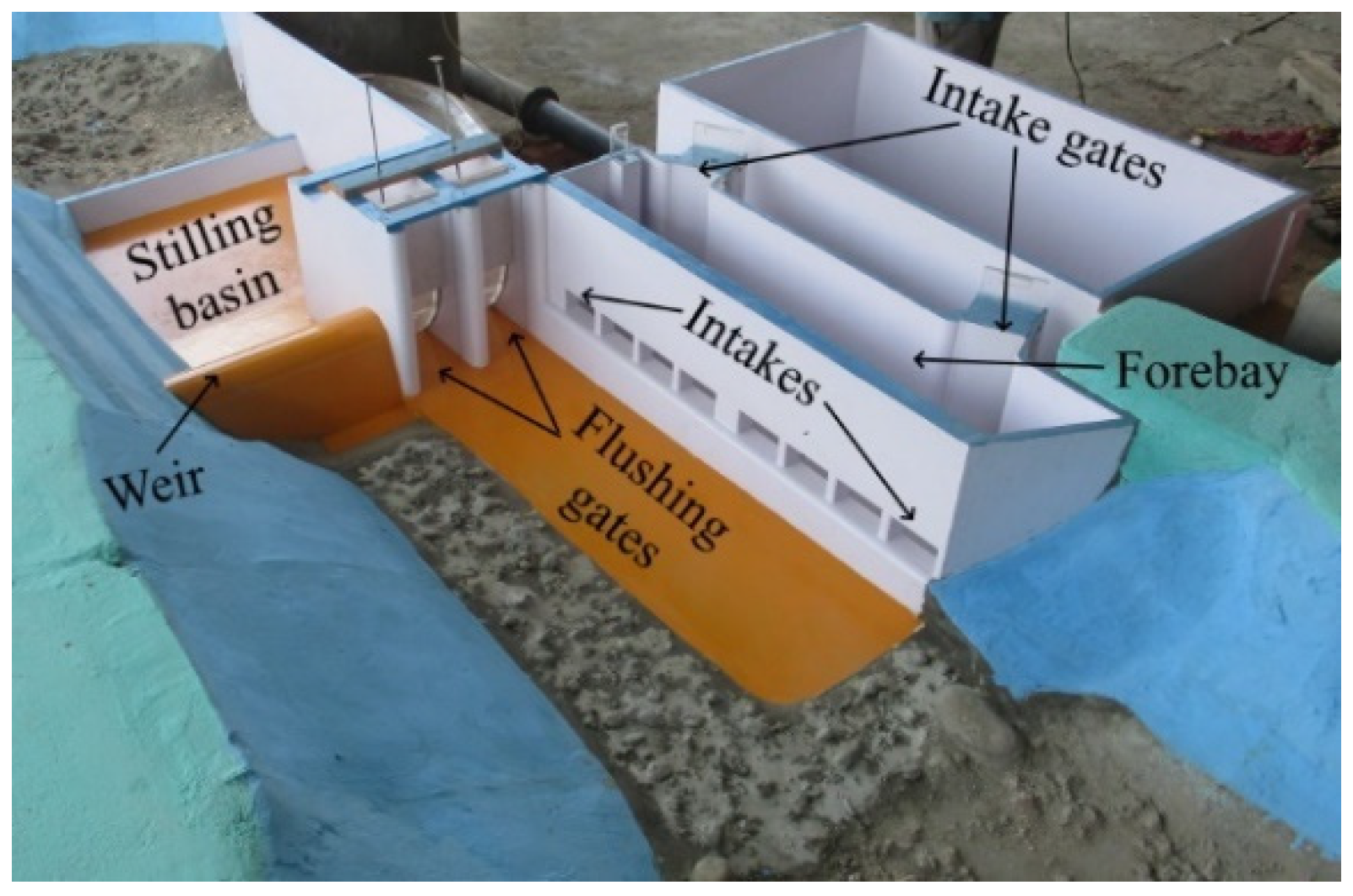
A physical hydraulic model of the headworks of a hydropower project in Khimti River of Nepal was selected to apply SfM technique in investigating flushing efficacy of headworks structures. Khimti River is a tributary of Tamakoshi River in Saptakoshi river basin. The Saptakoshi River is one of the tributaries of the Ganges River. The study area covered about 250 m reach of Khimti River upstream of the weir axis (
Figure 5). The model was built as an undistorted fixed bed model on a scale of 1:40 using the Froude’s Model Law. The headworks design consisted of a free flow type gravity weir, two bed load sluices, a side intake with eight orifices and a forebay from where water is diverted towards settling basins through two gated inlet orifices. A general arrangement of the headwork is as shown in
Figure 6. Since Khimti River is a typical Himalayan river with steep gradient, the hydropower plant was designed as run-off-river type. In such headworks arrangement, the pool created upstream of the diversion weir is normally insignificant and gets filled with the incoming sediment in very short time-span of operation. So, the designed headworks arrangement should be able to flush the sediment deposits around the intake area in order to avoid entry of bed sediments into the intakes. Regarding this, one of the main objectives of the model study was to ensure the capability of flushing gates to clean the deposited sediments from area around the intake upstream of the diversion weir. Since the partial opening of flushing gates in normal operation condition could not stop sedimentation in front of intakes, free flushing with annual flood discharge was tested in the model.
In order to speed up the sedimentation process, the river upstream of the weir was initially filled with bed sediment up to the sill level of intake orifices. The sand used for representing the bed load had median particle diameter (
d50) of 1.5 mm,
d10 = 0.5 mm and
d90 = 10 mm. The sediment fed with the inflow discharge during the test also had the same composition. The model was run under normal operating conditions for 12 min (1.3 h in prototype) simulating a river discharge of 14.4 L/s (equivalent to annual flood with the magnitude of 146 m
3/s in prototype) with sediment feeding at the rate of 0.580 kg/min which corresponds to sediment concentration of 671 ppm in the flow. Then both flushing gates were opened to allow free gravity flushing of the bed sediment with the annual flood discharge for 38 min (4 h in prototype). Initial bed before flushing and final bed after flushing were photographed and a dense point cloud for each scenario was produced in prototype scale using SfM technique in reference to 8 GCPs defined over the study area. The quality and size of dense point clouds produced with their respective processing times are presented in
Table 3. The DEMs generated from the dense point clouds of the two scenarios are shown in
Figure 7.
Errors in reproducing both the locations of GCPs and linear distances were calculated to be below 2 mm in the model as shown in
Figure 8 and
Table 4 respectively. Finally, flushing scenario was quantified by analysing the dense point clouds in CloudCompare software. Evaluating volume changes among dense point clouds for given scenarios, about 88% of sum of deposited sediment volume and volume of sediment fed was found to be flushed successfully keeping the area around the intake clean from sediment deposits. The flushed volume of sediment was estimated as a volume difference between dense cloud for initial bed before flushing and that for final bed after flushing in addition to the volume of sediment fed during the experiment. The estimated flushed volume of sediment in model scale was 0.1602 m
3 against the measured volume of 0.162 m
3 with only 1% of discrepancy.
In this way, the SfM technique helped to precisely quantify the bed control near intake structure in physical model studies. The SfM technique was also useful in recording spatial distribution of the sediment deposits remained upstream of the headworks after flushing, which was very useful information for the designer to identify the passive zones not cleaned by the flushing operation and to further modify, if required, the components of headworks structure to improve its overall performance. However, in this test the flushing operation was satisfactorily successful as 88% of the sediment were flushed downstream and the area around the intake was clean of sediment deposit.
3.3. Case Study III: Measurement of Flushing Cone Volume
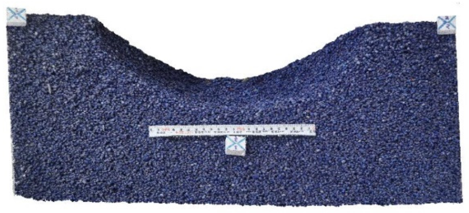
Finally, the SfM technique was applied on small scale flume experiments to investigate scour holes, commonly called as flushing cones, created by pressurized flushing of sediment deposit through a bottom outlet under steady flow conditions. The experimental setup consisted of a 0.6 m wide horizontal flume with a 50 mm wide rectangular orifice, the opening height of which was variable, at the centre of the flume. The sill of the orifice was 60 mm above the flume bed. A 120 mm thick layer of plastic grains representing sediment in the model were filled before the tests. Then a desired discharge was supplied into the flume without disturbing the filled sediment layer. When the water surface reached desired level, the bottom outlet was opened for desired opening height, which was meant to maintain the selected water level for the selected discharge, and pressurized flushing of the deposits were allowed to form a flushing cone. Once the flushing cone upstream of the outlet reached an equilibrium, the gate was closed and the flume was drained slowly without disturbing the cone. Then the flushing cone was measured manually with a millimeter precise point gauge as well as using SfM technique. Total 7 tests were carried out for different combination of discharge, water level and opening height of the outlet as listed in
Table 5.
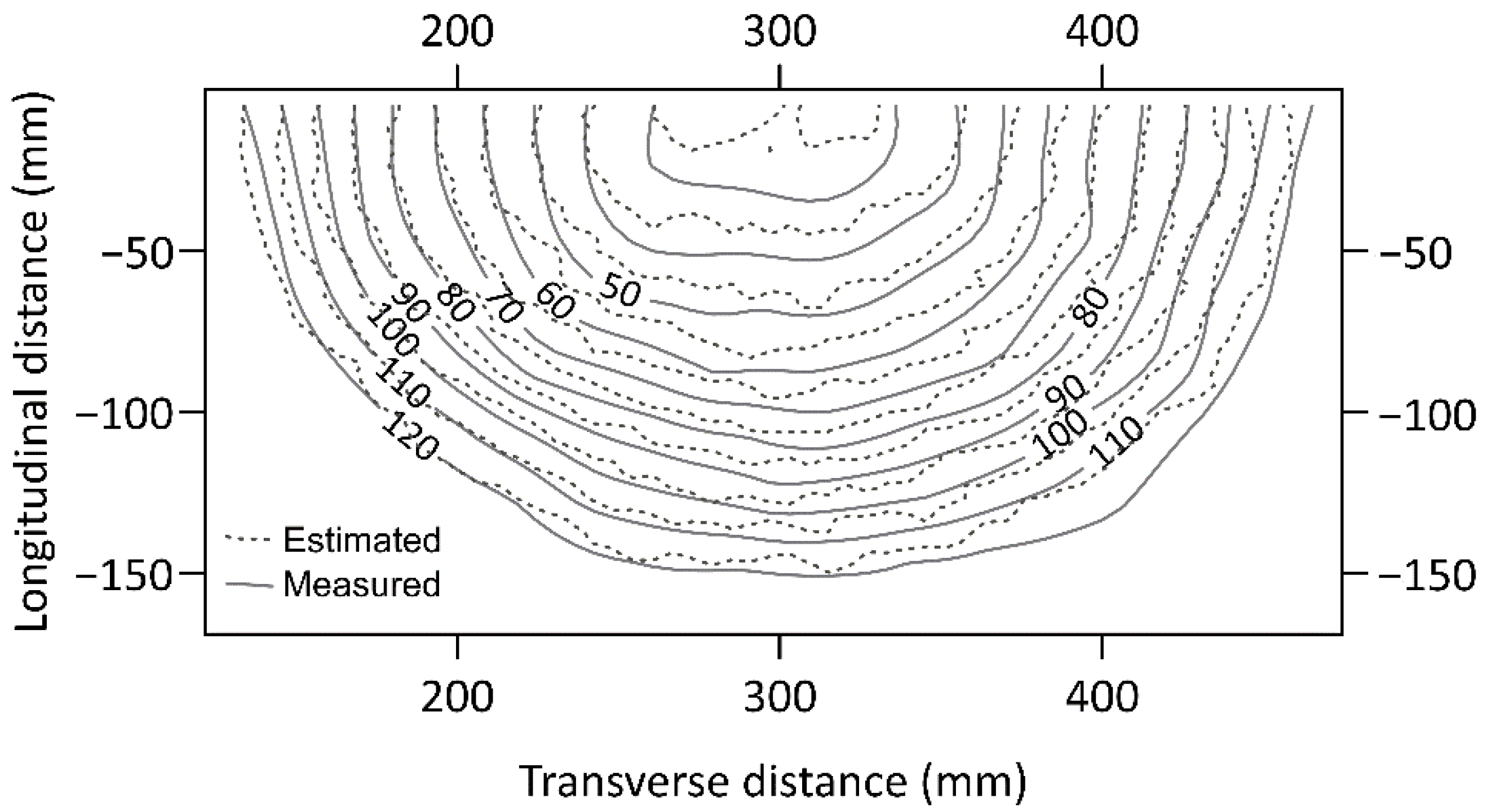
Since it was a small-scale flume test, high quality dense clouds were produced expecting better accuracy. For example, the dense point cloud for Test no. 3 is shown in
Figure 9. The contour plot of flushing cone for Test no. 3 produced by SfM superimposed on that produced by manual measurements is presented in
Figure 10. It shows that the flushing cone reproduced with SfM technique is comparable against the one produced by manual measurement.
The size of dense point cloud for each test and their respective processing time is shown in
Table 6. The volumes of flushing cones measured manually were compared with volumes of respective cones estimated by SfM technique as shown in
Table 5. The absolute discrepancy between measured and estimated volumes for all the tests were below 5% of the measured volume.
After achieving satisfactory precision from the SfM technique for such experiments, it was further applied in similar tests to produce high resolution point clouds of flushing cones which was utilized for precisely estimating dimensions and volume of flushing cones. A number of tests were carried out with varying water level, discharge, opening height of outlet, thickness of sediment deposit and density of sediment materials. The results from the experiments were used to develop empirical relations to predict the length and volume of flushing cone for relevant input parameters.


