Article

Surface Water Temperature Predictions at a Mid-Latitude Reservoir under Long-Term Climate Change Impacts Using a Deep Neural Network Coupled with a Transfer Learning Approach

1
Institute for Rural Engineering, National Agriculture & Food Research Organization (NARO), 2-1-6 Kannondai, Tukuba City, Ibaraki 305-8609, Japan
2
Center for Water Cycle, Marine Environment, and Disaster Management, Kumamoto University, 2-39-1 Kurokami, Kumamoto 860-8555, Japan
3
ARK Information Systems, INC, 4-2 Gobancho, Chiyoda-ku, Tokyo 102-0076, Japan
*
Author to whom correspondence should be addressed.
Water 2021, 13(8), 1109; https://doi.org/10.3390/w13081109
Submission received: 5 March 2021 / Revised: 13 April 2021 / Accepted: 14 April 2021 / Published: 17 April 2021
(This article belongs to the Special Issue Machine Learning for Hydro-Systems)

Abstract

:
Long-term climate change may strongly affect the aquatic environment in mid-latitude water resources. In particular, it can be demonstrated that temporal variations in surface water temperature in a reservoir have strong responses to air temperature. We adopted deep neural networks (DNNs) to understand the long-term relationships between air temperature and surface water temperature, because DNNs can easily deal with nonlinear data, including uncertainties, that are obtained in complicated climate and aquatic systems. In general, DNNs cannot appropriately predict unexperienced data (i.e., out-of-range training data), such as future water temperature. To improve this limitation, our idea is to introduce a transfer learning (TL) approach. The observed data were used to train a DNN-based model. Continuous data (i.e., air temperature) ranging over 150 years to pre-training to climate change, which were obtained from climate models and include a downscaling model, were used to predict past and future surface water temperatures in the reservoir. The results showed that the DNN-based model with the TL approach was able to approximately predict based on the difference between past and future air temperatures. The model suggested that the occurrences in the highest water temperature increased, and the occurrences in the lowest water temperature decreased in the future predictions.

1. Introduction

Global warming may strongly affect mid-latitude regions by the end of the twenty-first century [1]. The increase in air temperature can potentially cause significant changes in aquatic environments, as well as result in frequent occurrences of water-related disasters in hydrological systems in the mid-latitude regions. For example, according to previous studies, Hokkaido (Japan), which is a mid-latitude region, might experience severe flood disasters due to an unexpected heavy rainfall event under the impact of future climatic changes [2,3]. However, the impact of global warming on aquatic environments in Hokkaido has rarely been studied as a specific region (e.g., Umeda and Ochiai [4]).
In general, past studies have reported the impacts of climatic change on the water temperature of water bodies, such as reservoirs and lakes, using a simple method with observed data. For example, a linear regression method was used to determine the relationship between lake water temperature and weather conditions, such as air temperature and sunlight [5,6]. Although the linear regression easily shows a trend of the dependent variable that responds to the independent variable, it inappropriately predicts the dependent variable when the independent variable has strong nonlinearity, such as meteorological and limnological data, including uncertainties from complex climatic factors and aquatic systems (e.g., Mudelsee [7]). Conversely, non-linear methods (e.g., deep neural networks (DNNs)) have been recently utilized in big-data sciences. DNNs can extract features even from data that include nonlinear patterns. Therefore, they can be used for accurate prediction once they are trained with a large number of nonlinear data [8]. In fact, certain studies applied the DNN to lakes in a continental subarctic climate in mid-latitude regions to predict water temperature profiles [9] and water quality [10].
However, DNNs cannot provide accurate predictions when they are applied to out-of-range training data. That is, DNNs present inferior results while performing extrapolation, despite being one of the useful interpolation schemes. For instance, even well-trained DNNs with observed data may not predict accurately if unexperienced data are used, such as future data on super typhoons projected by an atmospheric general circulation model (GCM). This is one of the disadvantages of DNNs. To overcome the disadvantages related to out-of-range predictions, we introduced a transfer learning (TL) approach [11] in DNNs, which may achieve appropriate predictions even with unexperienced data. The TL approach proposes that a model pre-trained with the source data having different features can be reused with the target data. The model based on the target data can consider the inherent features of the source data. A few studies have employed the TL approach for flood predictions in hydrological systems [12,13]. However, the TL approach has not been applied to aquatic systems, such as reservoirs and lakes.
Our unique aim is to estimate the local impacts of long-term climate change on reservoir environments (e.g., water temperature) using a DNN-implemented model coupled with the TL approach. Therefore, our study first acquired locally downscaled data in a mid-latitude area from past and future GCM projections. Then, we validated the DNN model with and without the TL approach using the observed data. Finally, past and future predictions using trained DNNs and downscaled data were performed to understand the trends between past and future surface water temperatures that are affected by climate change.

2. Materials and Methods

This section describes the data acquisition for observation and downscaled projections by a GCM, features of the DNN model and the TL approach, model evaluations, procedures, and computational setups.

2.1. Data Acquisition

2.1.1. Target Site and Observed Data

In situ data (observed data) for surface water and air temperatures were obtained from the reservoir of the Tokachi Dam (hereafter Tokachi Dam reservoir) (43.2402° N, 142.9388° E), which is exposed to a humid subarctic climate, and is located in an upstream area of the Tokachi River watershed in the southeast portion of Hokkaido (Figure 1). The reservoir has a narrow and deep V-type shape along the continuous mountains and the catchment area of 592.0 km2. It is approximately 4 km long, 0.5 km wide, and 80 m deep when it is at total water capacity (112,000,000 m3), and has a large flood surface area (4.2 km2). We obtained the monthly meteorological data and surface water temperature (–1–0 m) from 1984 to 2020, which was spontaneously measured between 10:00 and 15:00. The surface water temperature was recorded as approximately 0   (e.g., 0.5 ) when ice cover appeared during winter. The number of data points was approximately 450. We assumed that the data could be representative of typical values in each month. Figure 2a shows the temporal variations in air and surface water temperatures observed near the levee of the Tokachi Dam reservoir. Scattered plots between both datasets indicate a moderate relationship with a linear regression of the coefficient of determination (R2), as shown in Figure 2b. Note that only air temperature is available as onsite weather data for about a 35-year observation period.
Another monthly dataset (surface water and air temperatures) from 2003 to 2018 was obtained from 18 reservoirs located in southwest Japan (Kyushu) for the pre-training process in the TL approach. The reservoir data were cyclically combined into one dataset based on an annual period. This rough treatment is acceptable, because DNNs usually learn patterns in time series data. The number of data points was approximately 3100. Note that the size, location, and surrounding environment of these 18 reservoirs were different from those of the Tokachi Dam reservoir; however, we assumed that the effect of air temperature on surface water temperature was greater than that of size, location, and the surrounding environment. The characteristics of the 18 reservoirs at Kyushu are shown in Appendix A.
Most observed data were publicly available in the database of dams in Japan [14]. Certain data were provided by the Hokkaido regional development bureau of the Ministry of Land, Infrastructure, Transport, and Tourism (MLIT) in Japan.

2.1.2. General Circulation Model and Weather Research and Forecast Model Data

The study used a 112 km grid with 48 vertical layers for the spatial data, and the sequential GCM data of 150 years for the temporal data, which were provided by running the Meteorological Research Institute coupled GCM version 3 [15,16]. Using the GCM data simulated for the past and future with the Representative Concentration Pathway (RCP) 8.5 scenario, we obtained a local dataset at the Tokachi Dam reservoir by means of dynamical downscaling. The local data were obtained from a regional circulation model, i.e., the Weather Research and Forecast (WRF) model [17,18], with a 9 km × 9 km grid, 40-layer vertical resolution, and hourly time interval. The data were obtained from a study of Ishida and Tanaka [19], in which the 150-year sequential meteorological data were simulated using two-step nested domain downscaling in the Tokachi River watershed with the setup of the Bougeault and Lacarrere scheme for planetary boundary layer parameterization, the Dudhia scheme for short-wave radiation parameterization, and the rapid and accurate radiative transfer scheme for long-wave radiation parameterization (refer to Ishida et al. [20] in detail). The data were classified into past data (1950−2005) and RCP 8.5-based future data (2006−2100) according to the computational setups for GCM data. Hereafter, the downscaled data are referred to as WRF data.
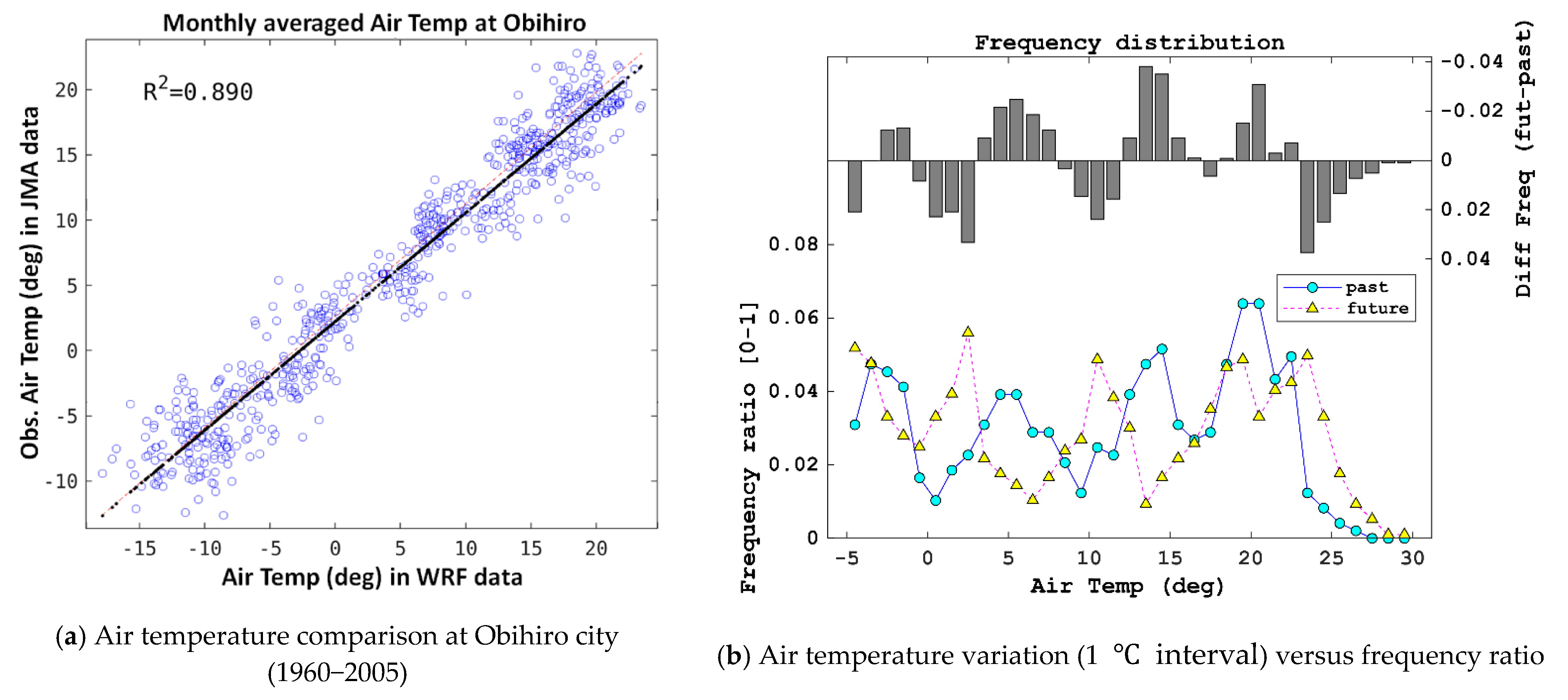
Long-term air temperature was calculated as monthly averaged data from the WRF data using only the data collected around mid-day (10:00−15:00) to approximately compare it to the collecting setup of observation. We performed a preliminary data analysis related to the reliability of the WRF data at the Tokachi River watershed and the monthly trends of past and future WRF data. Figure 3a shows a comparison of monthly averaged air temperatures during the period of 1960−2005 between the WRF data and observed data at Obihiro City, which is approximately 50 km south of the Tokachi Dam reservoir. The observed data at the Obihiro meteorological station were obtained from the past weather database of the Japan Meteorological Agency (JMA) [21]. While comparing the observed and WRF data, it can be noted that the data from the Obihiro meteorological station are better than that from the Tokachi Dam reservoir, because the station recorded relatively long-term data at the Tokachi River watershed. The past WRF data (1960−2005) averaged over each month showed a strong relationship with the data observed by the JMA. In addition, the difference between the past and future WRF data at Tokachi Dam reservoir is shown with respect to months (Figure 3b). It can be observed that the frequency of the higher air temperatures in the future WRF data obviously increase. Note that no bias correction was applied.

2.2. Long Short-Term Memory Model

We employed a long short-term memory (LSTM) architecture [22] as a DNN. The LSTM algorithm is a class of recurrent neural networks (RNNs) [23], which is a powerful tool that deals with continuous data. The LSTM is an advanced RNN that can memorize long-term trends in continuous data by solving the problems of RNN, such as vanishing and exploding gradients. Our deep learning model involves LSTM as a training and prediction engine (hereafter, referred to as the LSTM model). The LSTM model structure consists of an LSTM layer, a fully connected layer, and two activation functions (Figure 4a). The activation function has two functions: hyperbolic tangent and sigmoid. The hyperbolic tangent function outputs a value ranging from −1 to 1 (i.e., f ( x ) = ( e x e x ) / ( e x + e x ) , where x = input data (−∞, ∞)). The sigmoid function can nonlinearly normalize the input data from zero to one (i.e., f ( x ) = 1 / ( 1 + e x ) , where x is the same as the previous variable). The LSTM model has several hyperparameters (e.g., the number of epochs and batch size) that we tuned in preliminary tests for the adaptation of input data. The setup of these hyperparameters is listed in Table 1. Detailed explanations for the LSTM model are provided in our previous study [24].

2.3. Transfer Learning (TL) Approach

The idea of the TL approach is to reuse a model that is trained on a certain (source) dataset (i.e., a pre-trained model) on a different (target) dataset. The features extracted from the pre-trained model can be passed to a new model that is trained using the target data by reusing parts of the pre-trained model (Figure 4b). As shown in Figure 4b, the TL approach in this study retrained only a fully connected layer 1000 times. The extracted features are appropriately adapted to the new model after the inner parameters in the new model are tuned. Therefore, the new model can involve features from the pre-trained model. Our previous study [13] demonstrated detailed practical use of the TL approach.

2.4. Evaluation

The accuracy of the LSTM model in the observed data (Step 2 in Figure 5) was evaluated using K-fold cross-validation [25]. We selected K = 10 for segmenting the data. Nine segments were used for training, and the remaining segment was used for prediction. This was repeated 10 times by changing the prediction segment. For quantitative error evaluation, the root mean square error (RMSE) and Nash–Sutcliffe efficiency coefficient (NSE) were employed, the equations of which are listed in Table 1.

2.5. Procedures and Setups of the Computation

The procedure of this study is as follows: (Step 1) data acquisition of the long-term WRF data and 35-year observed data at the Tokachi Dam reservoir; (Step 2) training and validation of the LSTM model with and without the TL approach; and (Step 3) presenting past and future predictions using WRF data. These steps are illustrated in Figure 5.
Step 1 is explained in Section 2.1.2. Step 2 required the observed data, described in Section 2.1.1, along with the LSTM model in Section 2.2, and the TL approach in Section 2.3. Reproducibility calculations were set up as follows: Case 0 for a linear regression method between surface water and air temperatures, Cases 1 and 2 for the LSTM model with and without additional input data, respectively, and Case 3 for the LSTM model coupled with the TL approach. Cases 2 and 3 added additional input data (i.e., air temperature difference within a time interval) to accurately capture the temporal patterns that changed dramatically. The details of the setup are listed in Table 2.
In Step 3, past and future predictions were conducted using the WRF data and trained LSTM models with cross-validation (Section 2.4.). Note that the models were trained using all observed data before the past and future predictions. The future predictions using future WRF data were separated into three periods—near-future (2006−2039), mid-future (2040−2069), and far-future (2070−2100) predictions—to gain a long-term trend of surface water temperatures when compared with those in past predictions.
Numerous uncertainties from long-term changes in water resources, including aquatic environments, usually require a variety of computational conditions in climate change modeling [26], which are impossible to set up in this study. Therefore, to simplify the model calculations, the following assumptions were considered:
  • air temperature strongly affects the surface water temperature;
  • the humid subarctic climate in the Tokachi River watershed (the target) changes into a humid subtropical climate at Kyushu (the source). Note that the TL approach possibly adjusts the source climate to the target climate, although past air temperature at the source was significantly higher than that at the target;
  • the effect of water level variations is involved in the variations of surface water temperature;
  • no sediment accumulation affects the topographical aspects of the reservoir;
  • no geological changes occur in the surrounding environments;
  • the effect of the presence or absence of ice cover is included in the values of the surface water temperature;
  • the effect of the air−water interaction on surface water temperature is homogeneous among lakes.
The program for the LSTM model was created using Python (version 3.6.4) incorporated with Python deep learning libraries in Keras [27].

3. Results

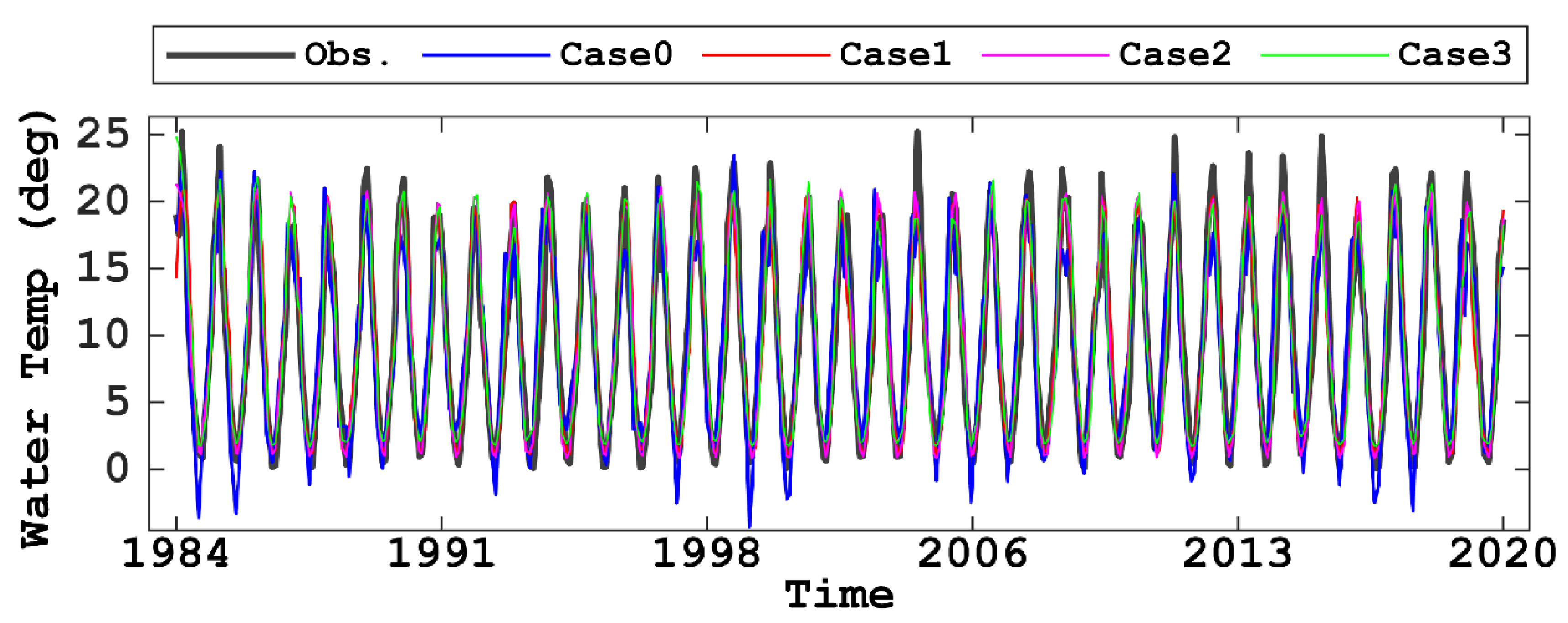
The validation of the LSTM model with the observed data was conducted in certain cases, including a linear fitting function (e.g., linear regression) as a reference. Note that the linear regression had cross-validation with 10-segment data (refer to Section 2.4.), as well as the LSTM model. Figure 6 illustrates the temporal variations of the surface water temperature in the re-productivity calculation cases when compared to the observed data for approximately 35 years. Case 0 shows an undershoot below zero, which indicates unreal surface water temperature values. Cases 1 and 2 have similar trends, and could not capture relatively larger water temperatures. The surface water temperature curve in Case 3 was shifted marginally upward from the lines observed for Cases 1 and 2. This was caused by the features of the water temperatures at Kyushu using the TL approach.
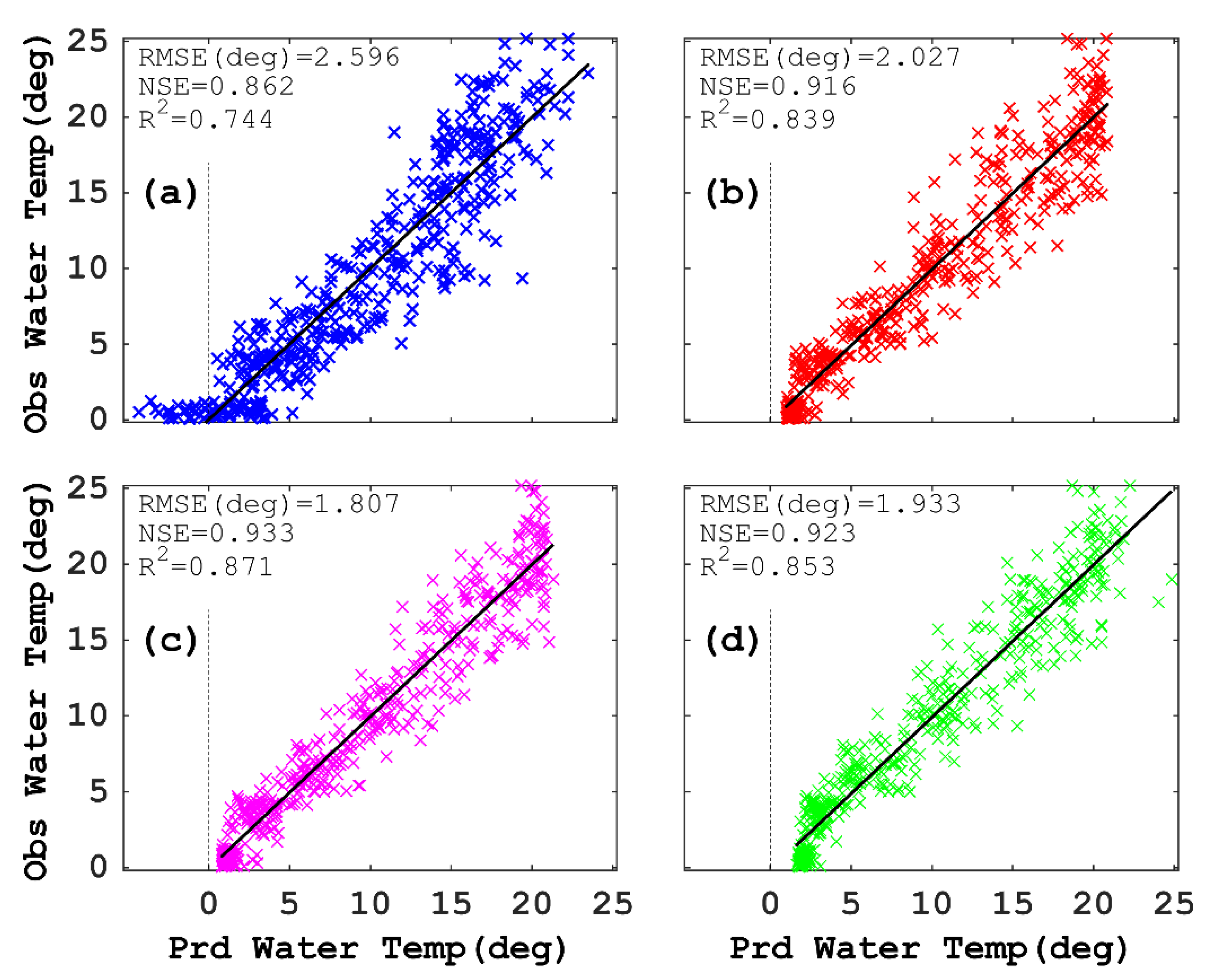
Figure 7 illustrates the relationship between the predicted and observed surface water temperatures with a regression line of R2 and the values of RMSE and NSE. Excluding Case 0, strong relationships were evident with R2 > 0.8 and NSE > 0.9. The prediction in Case 2 was marginally better than that in Case 1, with a 10% reduction in RMSE because of the additional input of the air−temperature difference within a time step. The prediction in Case 3 was marginally worse than that in Case 2, with a 7% increase in RMSE because of the marginal effect of inherent features of surface water temperatures at Kyushu. However, Case 3 was able to predict higher surface water temperatures in over 18 than Case 2 (Figure 7c,d). This feature suggests that Case 3 can be beneficial for a future prediction under the global warming impacts.
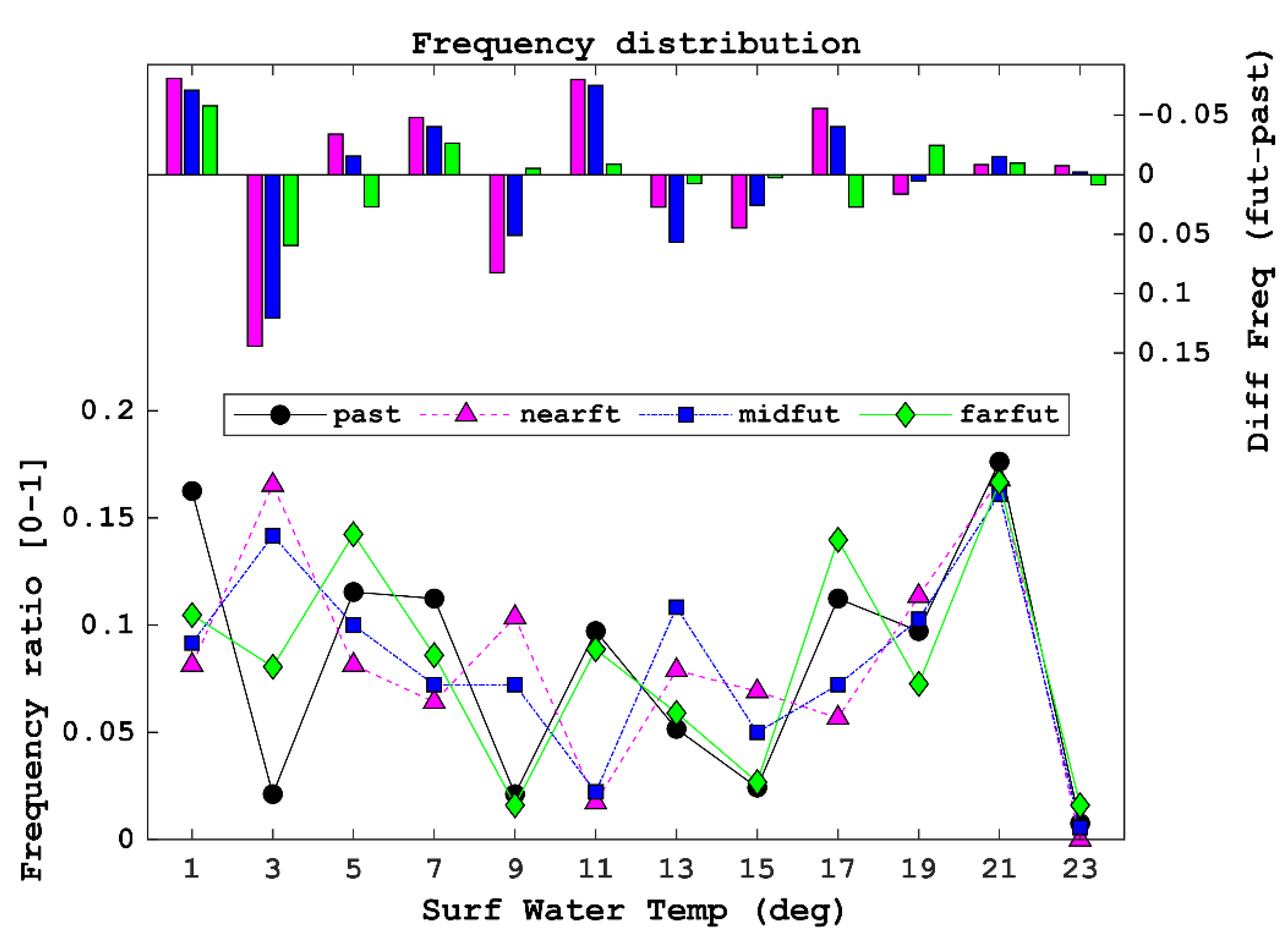
We estimated the impacts of climate change on surface water temperatures in the Tokachi Dam reservoir using past and future WRF data and the LSTM model, which was verified with the observed data. First, the Case 2 model was utilized for both WRF datasets. Second, the Case 3 model was applied to future WRF data based on the assumption that the humid subarctic climate changes to a humid subtropical climate. Note that the Case 3 model was not applied to past WRF data. Future predictions of surface water temperature with the RCP 8.5-based WRF data were separated into three periods (near, mid, and far future periods). We computed the number of water temperature values that were segmented in 2   intervals as a frequency ratio, which is the number of water temperature values divided by the total number of values. This ratio indicates the segmented water temperature values that increase or decrease during the three future periods and the past period. The difference in the frequency ratios between the past and the three future periods was also calculated to show positive and negative trends from past surface water temperatures. As observed in Figure 8, the Case 2 model shows that lower water temperatures (1−3   ) in the three futures had an opposite trend to that in the past. This temperature range suggests that winter ice covers may have melted down, possibly due to the impact of climate change (i.e., the increase of air temperature). The ratios in middle-range temperatures (5−17 ) were scattered up and down weakly as the water temperature increased. High water temperatures showed minimal differences among the four ratios. According to these results, the ratios in the far future prediction were significantly weaker than those of the other future periods, which was similar to past ratios. This far future prediction is not consistent with the significant increase in air temperature in the future WRF data, as shown in Figure 3b.
We assumed that this inconsistency could be caused by the nature of DNNs, which can predict only within the range of trained values. Therefore, the Case 3 model prediction was conducted to overcome this limitation of DNNs. Figure 9 shows that lower water temperatures (1−3   ) in the three future ratios had an inverse trend to the past ratio, similar to the result of the Case 2 model. The middle range of water temperatures indicates that the different ratios of the three futures were considerably scattered, which was similar to the other model. However, the difference ratios at the highest water temperature were positive. These results support the trend ratio of future air temperature values. In particular, the ratio of the far future prediction was high in the extreme ranges of water temperature (i.e., 1 and 23 ).
In addition, we introduced a net heat-related factor to quantify the contribution of the Case 3 model to an appropriate future prediction under the effect of global warming. The net heat-related factor was defined in this study as the accumulation of the differences of the frequency ratio between future and past predictions that was multiplied by surface water temperature from 1 to 23 (i.e., i ( D F i · T i ) , where DF = future – past in the frequency ratio and T = surface water temperature) among the three future periods. In Figure 8, the Case 2 model was adopted as the pre-trained model to the future WRF data; on the other hand, the Case 3 model in Figure 9, to which the TL approach was implemented, was applied for the future WRF data (Table 3). The net heat-related factors in Figure 9 obviously were increased among the three future periods, rather than those in Figure 8 (Table 3). This suggests that the Case 3 model with the TL approach was more appropriate for future predictions under the effect of global warming.

4. Discussion

The prediction of surface water temperature using the LSTM model was accurate based on the quantitative evaluation of R2 and NSE (refer to Figure 7). While comparing the accuracy with other studies, our RMSEs (1.8–2.0 ) were comparable to the outputs from a single DNN, as used in past studies [9,28], although their computational setups were different from ours in terms of the amount of data and the target of water temperature profiles. Therefore, our LSTM model may be quantitatively reliable when considering the availability of only a few reports in lake and reservoir environment studies.
The water temperature trends under long-term climate change impacts have been revealed in limnology using relatively long observed data [5,6]. A simplified physical model (e.g., a vertical−longitudinal dimension hydrodynamic model) simulated the future trends using a GCM projection (e.g., the model proposed by Modiri-Gharehveran et al. [29]). The simplified model simulated for a short-term period based on future meteorological forcing, including the impact of climate change. However, continuous long simulations have not been performed, potentially because of the expensive computational costs and the lack of an adjustment scheme for observed data (e.g., data assimilation) for unexperienced events (i.e., future water temperatures). Therefore, DNNs with the TL approach (Case 3 model) are more realistic and practical at this stage for the prediction of future climate change impacts.
In general, DNNs must be first trained with known data, and then can be used to predict unknown data based on the patterns observed from the training data. Therefore, DNNs appear to be an interpolation scheme that estimate within the range between the maximum and minimum values in the training data. This is a limitation of the DNNs in our study, because surface water temperatures are unknown in future periods of climate change. Our study marginally extended the limitation, even within the same range of training data by introducing the TL approach to DNNs. However, the predicted surface water temperatures were still constrained by the range of the training data. Therefore, the maximum and minimum values of the setup affect the DNN predictions. For a more realistic setup of the range, physical models (e.g., a hydrodynamic model) that are exposed to future climate change [30] can be used. The physical models may simulate only extreme events that provide maximum and minimum water temperatures, because physical models usually incur high computational costs for long-term simulations. Although choosing appropriate maximum and minimum values with physical models is beyond the scope of our study, it should be considered in future work.
Furthermore, physics-guided DNNs that incorporate a heat balance embedded physical model as an internal mode have recently been developed [9,28]. The accuracy of their DNNs in water temperature was satisfied with smaller RMSEs (approximately 1.0 ); however, the reliability of long-term simulations for 100 years is unknown. This is because an accurate physical model in limnology generally uses a data assimilation scheme that constrains simulated outputs to observed data. In fact, future water temperatures affected by future climate change are unknown. Therefore, a long-term simulation by a physical module may cause the accumulated errors from the difference between predicted values and virtual observed ones that we do not know in reality in future.

5. Conclusions

To understand the impacts of long-term climate change on mid-latitude reservoir environments, we conducted past and future predictions of surface water temperature using locally downscaled climate data from GCM projections (RCP8.5), along with the LSTM model coupled with the TL approach. Our study provides the following findings:
  • The LSTM model that was validated with the observed data achieved accurate reproducibility calculations with R2 > 0.8 and NSE > 0.9. In particular, Case 2 with two input datasets, i.e., air temperature and difference in air temperature, was marginally better than the other cases.
  • Past and future predictions with locally downscaled data showed that the LSTM model with the TL approach (Case 3 model) was more realistic for future prediction than that without the TL approach based on the difference between past and future air temperatures. The Case 3 model suggested that the frequency ratios with respect to the predicted surface water temperature were increased in the highest range of water temperature and decreased in the lowest range, because the model predicted higher water temperatures.
We proposed a method (a DNN with the TL approach) that improved the disadvantage of DNNs and was implemented with unexperienced data (i.e., surface water temperature in the future). However, DNNs are still constrained by the maximum and minimum ranges of training data (i.e., the observed surface water temperature in our study). Physical models may provide an appropriate range of unexperienced data based on physical processes driven by future GCM projections. Therefore, DNNs coupled with physical models may be required in future work.

Author Contributions

Conceptualization and methodology, N.K.; software, D.B.; validation, N.K., K.I., and D.B.; formal analysis, N.K.; investigation, resources and data curation, N.K. and K.I.; writing—original draft preparation, N.K.; writing—review and editing, N.K., K.I., and D.B.; visualization, N.K.; supervision, N.K.; project administration, N.K.; funding acquisition, N.K. and K.I. All authors have read and agreed to the published version of the manuscript.

Funding

This research was funded by the Integrated Research Program for Advancing Climate Models, TOUGOU (grant number: JPMXD0717935498), the Environment Research and Technology Development Fund (grant number: JPMEERF20S11803), and the Sumitomo Foundation (grant number: 193094).

Institutional Review Board Statement

Not applicable.

Informed Consent Statement

Not applicable.

Data Availability Statement

All data analyzed in this study are included in this article.

Acknowledgments

We greatly appreciate Yuya Kino (the ARK Information Systems, Japan) for his helpful advice on the model uses, and the Hokkaido branch of MLIT Japan for giving us parts of observed data at the Tokachi Dam reservoir.

Conflicts of Interest

The authors declare no conflict of interests.

Appendix A

We obtained observed data from 18 reservoirs at Kyushu for a source in the TL approach. The 18 datasets include monthly data of air temperature and surface water temperature. Each dataset was connected with other datasets based on an annual cycle, and then one sequential dataset was created. However, the created data are not time series data, although they have seasonal characteristics. Figure A1a illustrates the temporal variations of air and surface water temperatures. The scattered plots between both datasets are shown in Figure A1b with a regression line of R2 (0.63). The characteristics of the 18 reservoirs are listed in Table A1.
Figure A1. Observed data for air temperature ( ) and surface water temperature ( ) at Kyushu: (a) temporal variations connected with an annual cycle between different datasets, and (b) the relationship between air and surface water temperatures with a linear regression line (R2 = 0.63).
Water 13 01109 g0a1
Table A1. Reservoir characteristics at Kyushu.
NameLocationTotal Capacity (m3)Surface Area
(km2)
Catchment Area
(km2)
Ayakita32.0975° N, 131.1422° E21,300,0000.82149.3
Ayanann32.0578° N, 131.1217° E38,000,0001.36101.0
Dokawa32.3553° N, 131.3453° E33,900,0001.54143.0
Hikawa32.5714° N, 130.7865° E6,300,0000.35 57.4
Hirowatari31.7167° N, 131.2675° E6,400,0000.3834.4
Houri32.7158° N, 131.5736° E5,774,0000.2845.2
Ichifusa32.3200° N, 131.0128° E40,200,0001.65157.8
Iwase31.9428° N, 131.1403° E57,000,0004.13354.0
Kawabe31.4450° N, 130.4456° E2,920,0000.2330.2
Matsuo32.2839° N, 131.3714° E45,202,0001.95304.1
Midorikawa32.6273° N, 130.9089° E46,000,0001.81359.0
Hase-miyazaki32.1458° N, 131.3403° E2,250,0000.1411.8
Nichinann31.6369° N, 131.2758° E6,000,0000.4159.2
Okita32.5506° N, 131.6192° E2,750,0000.278.8
Tachibana32.1322° N, 131.2700° E10,000,0000.2970.5
Tashirobae32.1367° N, 131.1197° E19,270,0001.02131.5
Turuta (old)31.9853° N, 130.4958° E123,000,0003.61805.0
Urita31.9267° N, 131.3086° E720,0000.074.4

References

  1. Intergovernmental Panel on Climate Change (IPCC) Climate Change 2014: Synthesis report. In Contribution of Working Groups I, II and III to the Fifth Assessment Report of the Intergovernmental Panel on Climate Change; Core writing team; Pachauri, R.K.; Meyer, L.A. (Eds.) IPCC: Geneva, Switzerland, 2014; 151p. [Google Scholar]
  2. Hoshino, T.; Yamada, T.J. Analysis of annual maximum precipitation over first-class river basins in Japan using a large-ensemble dataset(d4PDF). J. JSCE Hydraul. Engr. 2018, 74, I_187–I_192. (In Japanese) [Google Scholar] [CrossRef]
  3. Kimura, N.; Kiri, H.; Kanada, S.; Kitagawa, I.; Yoshinaga, I.; Aiki, H. Flood simulations in mid-latitude agricultural land using regional current and future extreme weathers. Water 2019, 11, 2421. [Google Scholar] [CrossRef] [Green Version]
  4. Umeda, M.; Ochiai, Y. Assessment of Water Quality Changes in Reservoirs in Japan Affected by Global Warming. J. Japan Soc. Civil Eng. 2012, 68, I_127–I_135. (In Japanese) [Google Scholar] [CrossRef]
  5. Ito, U.; Oda, S.; Momii, K. Global warming and heat-feature change in Lake Ikeda. In Proceedings of the Annual Meeting of Japan Society of Hydrology and Water Resources, Miyazaki, Japan, 25–28 September 2014. (In Japanese). [Google Scholar]
  6. Lewis, W.M.; McCutchan, J.H.; Roberson, J. Effects of climatic change on temperature and thermal structure of a mountain reservoir. Water Resour. Res. 2019, 55, 1988–1999. [Google Scholar] [CrossRef]
  7. Mudelsee, M. Trend analysis of climate time series: A review of methods. Earth Sci. Rev. 2019, 190, 310–322. [Google Scholar] [CrossRef]
  8. LeCun, Y.; Bengio, Y.; Hinton, G. Deep learning. Nature 2015, 521, 436–444. [Google Scholar] [CrossRef] [PubMed]
  9. Read, J.S.; Jia, X.; Willard, J.; Appling, A.P.; Zwart, J.A.; Oliver, S.K.; Karpatne, A.; Hansen, G.J.; Hanson, P.C.; Watkins, W.; et al. Process-guided deep learning predictions of lake water temperature. Water Resour. Res. 2019, 55, 9173–9190. [Google Scholar] [CrossRef] [Green Version]
  10. Peterson, K.T.; Sagan, V.; Sloan, J.J. Deep learning-based water quality estimation and anomaly detection using Landsat-8/ Sentinel-2 virtual constellation and cloud computing. GISci. Remote Sens. 2020, 57, 510–525. [Google Scholar] [CrossRef]
  11. Pratt, L.Y. Discriminability-based transfer between neural networks. In Proceedings of the Conference of the Advances in NIPS 5, Denver, CO, USA, 30 November–3 December 1992; pp. 154–196. [Google Scholar]
  12. Kratzert, F.; Klotz, D.; Brenner, C.; Schulz, K.; Herrnegger, M. Rainfall–runoff modelling using long short-term memory (LSTM) networks. Hydrol. Earth Syst. Sci. 2018, 22, 6005–6022. [Google Scholar] [CrossRef] [Green Version]
  13. Kimura, N.; Yoshinaga, I.; Sekijima, K.; Azechi, I.; Baba, D. Convolutional neural network coupled with a transfer-learning approach for time-series flood predictions. Water 2020, 12, 96. [Google Scholar] [CrossRef] [Green Version]
  14. Database of Dams in Japan. Available online: http://mudam.nilim.go.jp/home (accessed on 28 February 2021). (In Japanese).
  15. Mizuta, R.; Yoshimura, H.; Murakami, H.; Matsueda, M.; Endo, H.; Ose, T.; Kamiguchi, K.; Hosaka, M.; Sugi, M.; Yukimoto, S.; et al. Climate simulations using MRI-AGCM3.2 with 20-km grid. J. Meteor. Soc. Japan 2012, 90A, 233–258. [Google Scholar] [CrossRef] [Green Version]
  16. Yukimoto, S.; Adachi, Y.; Hosaka, M.; Sskami, T.; Yoshimura, H.; Hirabara, M.; Tanaka, T.Y.; Shindo, E.; Tsujino, H.; Deushi, M.; et al. A new global climate model of the meteorological research institute: MRI-CGCM3—Model description and basic performance. J. Meteor. Soc. Japan 2012, 90A, 23–64. [Google Scholar] [CrossRef] [Green Version]
  17. Weather Research and Forecasting (WRF) Model. Available online: https://www.mmm.ucar.edu/weather-research-and-forecasting-model (accessed on 28 February 2021).
  18. Shamarock, W.C.; Klemp, J.B.; Dudhia, J.; Gill, D.O.; Barker, D.M.; Duda, M.G.; Wang, W.; Powers, J.G. A Description of the Advanced Research WRF Version 3; NCAR Technical Note: Boulder, CO, USA, 2008. [Google Scholar] [CrossRef]
  19. Ishida, K.; Tanaka, K. Analysis of future changes in precipitation over watersheds in the Hokkaido region, Japan by means of dynamical downscaling. In Proceedings of the Poster, AGU Fall Meeting 2019, San Francisco, CA, USA, 9–13 December 2019. [Google Scholar]
  20. Ishida, K.; Tanaka, K.; Hama, T. Sensitivity analysis of convective parameterizations of a regional climate model in higher-resolution domains for long-term precipitation reconstruction. J. Water Clim. Chang. 2020, 11, 1467–1480. [Google Scholar] [CrossRef]
  21. Past Weather Database. Available online: http://www.data.jma.go.jp/gmd/risk/obsdl/index.php (accessed on 28 February 2021). (In Japanese).
  22. Hochreiter, P.; Schmidhuber, J. Long short-term memory. Neural Comput. 1997, 9, 1735–1780. [Google Scholar] [CrossRef]
  23. Hopfield, J.J. Neural networks and physical systems with emergent collective computational abilities. Proc. Natl. Acad. Sci. USA 1982, 79, 2554–2558. [Google Scholar] [CrossRef] [PubMed] [Green Version]
  24. Kimura, N.; Yoshinaga, I.; Sekijima, K.; Azechi, I.; Kiri, H.; Baba, D. Recurrent neural network predictions for water levels at drainage pumping stations in an agricultural lowland. Japan Agr. Res. Quart. 2021, 55. [Google Scholar] [CrossRef]
  25. Geisser, S. Predictive Inference: An Introduction, Mono-Graphs on Statistics and Applied Probability 55; Chapman and Hall: NewYork, NY, USA, 1993; 240p. [Google Scholar]
  26. Teegavarapu, R.S.V. Modeling climate change uncertainties in water resources management models. Environ. Modell. Software 2010, 25, 1261–1265. [Google Scholar] [CrossRef]
  27. Keras. Available online: http://keras.io/ (accessed on 28 February 2021).
  28. Jia, X.; Willard, J.; Karpatne, A.; Read, J.S.; Zwart, J.; Steinbach, M.; Kumar, V. Physics guided RNNs for modeling dynamical systems: A case study in simulating lake temperature profiles. In Proceedings of the 2019 SIAM International Conference on Data Mining, Calgary, AB, Canada, 2–4 May 2019; pp. 558–566. [Google Scholar] [CrossRef] [Green Version]
  29. Modiri-Gharehveran, M.; Etemad-Shahidi, A.; Jabbari, E. Effects of climate change on the thermal regime of a reservoir. Proceedings of the Institution of Civil Engineers. Water Manag. 2014, 167, 601–811. [Google Scholar] [CrossRef] [Green Version]
  30. Mi, C.; Shatwell, T.; Ma, J.; Xu, Y.; Su, F.; Rinke, K. Ensemble warming projections in Germany’s largest drinking water reservoir and potential adaptation strategies. Sci. Total Environ. 2020, 748, 141366. [Google Scholar] [CrossRef] [PubMed]
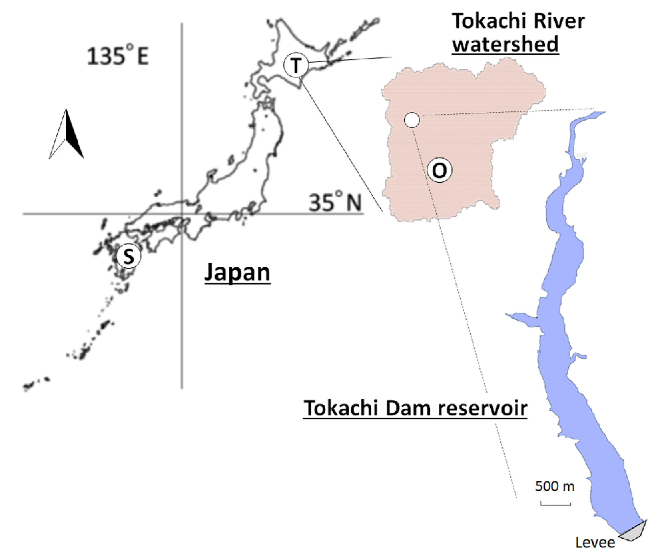
Figure 1. Maps of the target area (T), the Tokachi River watershed, and a target reservoir, i.e., the Tokachi Dam reservoir, where (O) is Obihiro, one of the meteorological stations of the Japan Meteorological Agency (JMA), and (S) is a source area at Kyushu.
Water 13 01109 g001
Figure 2. Observed data for air temperature ( ) and surface water temperature ( ) at Tokachi Dam reservoir: (a) temporal variations and (b) the relationship between air and surface water temperatures with a linear regression line (R2 = 0.75).
Water 13 01109 g002
Figure 3. Air temperature values in Weather Research and Forecasting (WRF) model data: (a) data reliability of past WRF data when compared with the observed data at the Obihiro meteorological station recorded by JMA, including a linear regression line of R2 (= 0.89); (b) variations in the frequency ratios of past and future WRF data and the frequency difference (future data subtracted by past data) with respect to air temperature with a 1   interval.
Water 13 01109 g003
Figure 4. Sketch of layer structures: (a) long short-term memory (LSTM); (b) transfer learning (TL) approach. Activ. func. = activation function (i.e., Activ. func. 1 = hyperbolic tangent; Activ. func. 2 = sigmoid).
Water 13 01109 g004
Figure 5. Sketch-like flowchart with maps in this study.
Water 13 01109 g005
Figure 6. Temporal variations during the period of May 1984–July 2020 of calculated and observed surface water temperatures ( ). In the legend in the figure, Obs. represents observation; moreover, the case names are as listed in Table 2.
Water 13 01109 g006
Figure 7. LSTM model outputs with the observed data in surface water temperature for four cases: (a) Case 0 as a reference (a linear regression), (b) Case 1, (c) Case 2, and (d) Case 3, showing a relation between Prd and Obs data with a linear regression line of R2. Dotted lines indicate zero Prd data. The root mean square error (RMSE) and Nash–Sutcliffe efficiency coefficient (NSE) are defined in Table 1. Prd = reproducibility calculation and Obs = observation.
Water 13 01109 g007
Figure 8. Comparisons between the past and the three future predictions in the Case 2 model for surface water temperature. Variations in the frequency ratios of the past and three future (near, mid, and far) predictions and the three differences (future data subtracted by past data) with respect to surface water temperature with 2   intervals.
Water 13 01109 g008
Figure 9. Comparisons between the past prediction in Case 2 and the three future predictions in the Case 3 model for surface water temperature, showing frequency ratios of the past and three future (near, mid, and far) predictions and the three differences (future data subtracted by past data) with respect to surface water temperature with 2   intervals.
Water 13 01109 g009
Table 1. Long short-term memory (LSTM) hyperparameters and other setups.
Hyperparameters
and Function
Values or EquationsRemarks
Number of LSTM layers1
Number of nodes20
Past and present time in input 6 to 0Time interval = month
Lead time in output1Time interval = month
Batch size100
Number of epochs1000Retaining the TL approach and has the same number
Learning rate0.01
Dropout rate0.0
ReproducibilityNone
OptimizerStochastic gradient descent (SGD)
Activation functionSigmoid
Hyperbolic tangent
Range from 0 to 1
Range from −1 to 1
Loss functionSum of squared residuals = 1 2 i = 1 N 1 ( V c i V o i ) 2 ci = model calculation, oi = observed data, N1 = the number of data
Error evaluation functionsRMSE =   1 N 1 i = 1 N 1 ( V c i V o i ) 2 Same as above
NSE =   1 i = 1 N 1 ( V c i V o i ) 2 / i = 1 N 1 ( V o i V o ) 2 Same as above, and <*> = average
Table 2. Re-productivity calculation cases.
NameModelInput DataTransfer Learning
Case 0Linear regressionAir temperatureNo
Case 1LSTMAir temperatureNo
Case 2LSTMAir temperature,
difference in air temperature
No
Case 3LSTMSame as aboveYes
Table 3. List of pre-training cases and net heat-related factors among three futures.
ResultPre-Trained Model Applied to
the Past WRF Data
Pre-Trained Model
Applied to
the Future WRF data
* Net Heat-Related Factor (Ratio °C)
Near FutureMid FutureFar Future
Figure 8Case 2Case 2−0.27−0.230.04
Figure 9Case 2Case 30.030.060.06
* The net heat-related factor was defined as the accumulation of differences of the frequency ratio between future and past predictions that was multiplied by surface water temperature from 1 to 23 .
Publisher’s Note: MDPI stays neutral with regard to jurisdictional claims in published maps and institutional affiliations.