1. Introduction
Refined medium and long-term runoff forecast technology is an important basis for the design, construction, and operation management of water conservancy and hydropower projects [
1,
2,
3]. It is a basic key technology to realize the scientific allocation of water resources and improve the utilization efficiency of water resources and has important supporting significance for the dispatching management and optimal allocation of water resources [
4,
5,
6]. With the rapid development of the social economy and the continuous improvement of science and technology, the ability of water resources regulation and control has been obviously improved. The practice of water resources regulation, such as unified regulation of basin water quantity, inter-basin water transfer, and joint regulation of super-large cascade reservoirs, has continued to advance, putting forward higher requirements for the forecast accuracy and forecast scale of medium and long-term runoff forecast. As such, its importance has become increasingly prominent [
7,
8,
9,
10]. In the unified regulation and management of water quantity in China’s Yangtze River, Yellow River, Pearl River and Huai River basins, medium and long-term runoff forecast are important scientific and theoretical bases for water resource allocation and regulation schemes, and the reliability, stability, and extensibility of the forecast results play a significant value [
11,
12].
However, monthly-seasonal-annual runoff forecast has always been a difficult point in hydrological science, both in theory and application. Compared with the short-term runoff forecast, the development is relatively slow and lags behind the actual production requirements [
13,
14]. It is of great theoretical and practical significance to establish a stable and reliable medium and long-term runoff forecast system by using fast-developing mathematics and computer technology while strengthening the collection and arrangement of basic data for runoff forecast [
15,
16].
In recent years, the fourth industrial revolution with Artificial Intelligence (AI) as its core has played an important role in hydrological forecasting, water resources regulation, and other fields. Among them, Machine Learning (ML) is an important branch of AI, and it is also a new discipline to study how to make computers learn rules from massive historical data through algorithms, so as to classify or predict new samples [
17]. The development of forecasting model in ML has experienced several significant milestone time nodes. In 1952, Arthur Samuel firstly gave the definition and operable program of ML [
18]. In 1958, Rosenblatt put forward the Perceptron Model which is the embryonic form of Artificial Neural Network (ANN) [
19]. However, it was not until Werbos applied BP algorithm to build multilayer perceptron in 1982 that ANN developed rapidly [
20]. In 1986, Quinlan proposed the earliest Decision Tree (DT), ID3 model [
21]. Since then, C4.5 [
22], CART [
23] and other DT algorithm have flourished. In 1995, ML ushered in a major breakthrough. The Support Vector Machine (SVM) [
24] presented by Vapnik and Cortes. It not only has a solid theoretical basis, but also has excellent experimental results. In 1999, Freund and Schapire put forward Adaptive Boosting (AdaBoost) [
25], and in 2001 Breiman proposed Random Forest (RF) [
26]. Both were based on DT theory and developed into representative algorithms of Boosting and Bagging [
27,
28], two important components of Ensemble Learning (EL).
When applying ML to medium and long-term runoff forecast, the first step is also the most important one, Feature Selection (FS), which is to extract accurate and appropriate features from the original data to the maximum extent by using relevant knowledge in the field of data analysis for the forecast model to achieve the best performance [
29,
30]. Due to the huge and messy data set, FS is a key step in building forecast models and also a highly iterative data preprocessing process [
31]. This includes two reasons. First, FS can avoid Dimension Disaster due to too many attributes, which has similar motivation to dimension reduction (such as PCA, SVD, LDA, etc.), that is, trying to reduce the number of features in the original data set. However, these two methods are different. Dimension reduction mainly obtains new features by recombining the original features, while FS is to select subsets from the original features without changing the original feature space. Second, FS reduces data noise and the training difficulty of learners while removing the irrelevant feature. For medium and long-term runoff forecast, the FS is to find out the feature matching relationships between monthly-seasonal-annual runoff sequences and the previous climate indexes and select a certain number of features with physical causes, strong mutual independence and accurate and stable forecast performances as forecast factors. Climate Indexes include but are not limited to Sea Surface Temperature, El Nino index, Subtropical High, Circulation Index, Polar Vortex, Trade Wind, Warm Pool, Ocean Dipole, Solar Flux, etc.
Compared with the physical-driven runoff forecast model, the data-driven runoff forecast model based on machine learning not only reduces the difficulty of understanding runoff mechanism and the complexity of modeling, but also provides a new idea for runoff forecasting due to its solid theoretical basis and good performance. Many hydrologists use ML and Big Data Mining methods, such as ANN [
32], SVM [
3], Extreme Learning Machine (ELM) [
33], Gradient Boosting Decision Tree (GBDT) [
34], Relevance Vector Machine (RVM) [
35], etc., to study and improve runoff forecast methods and models, to improve their ability to understand, predict and apply the evolution law of runoff phenomena.
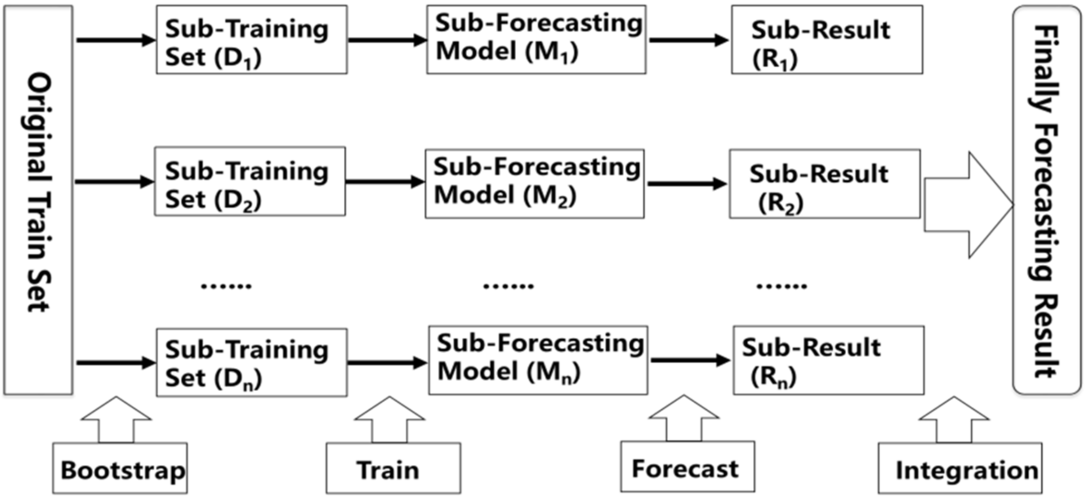
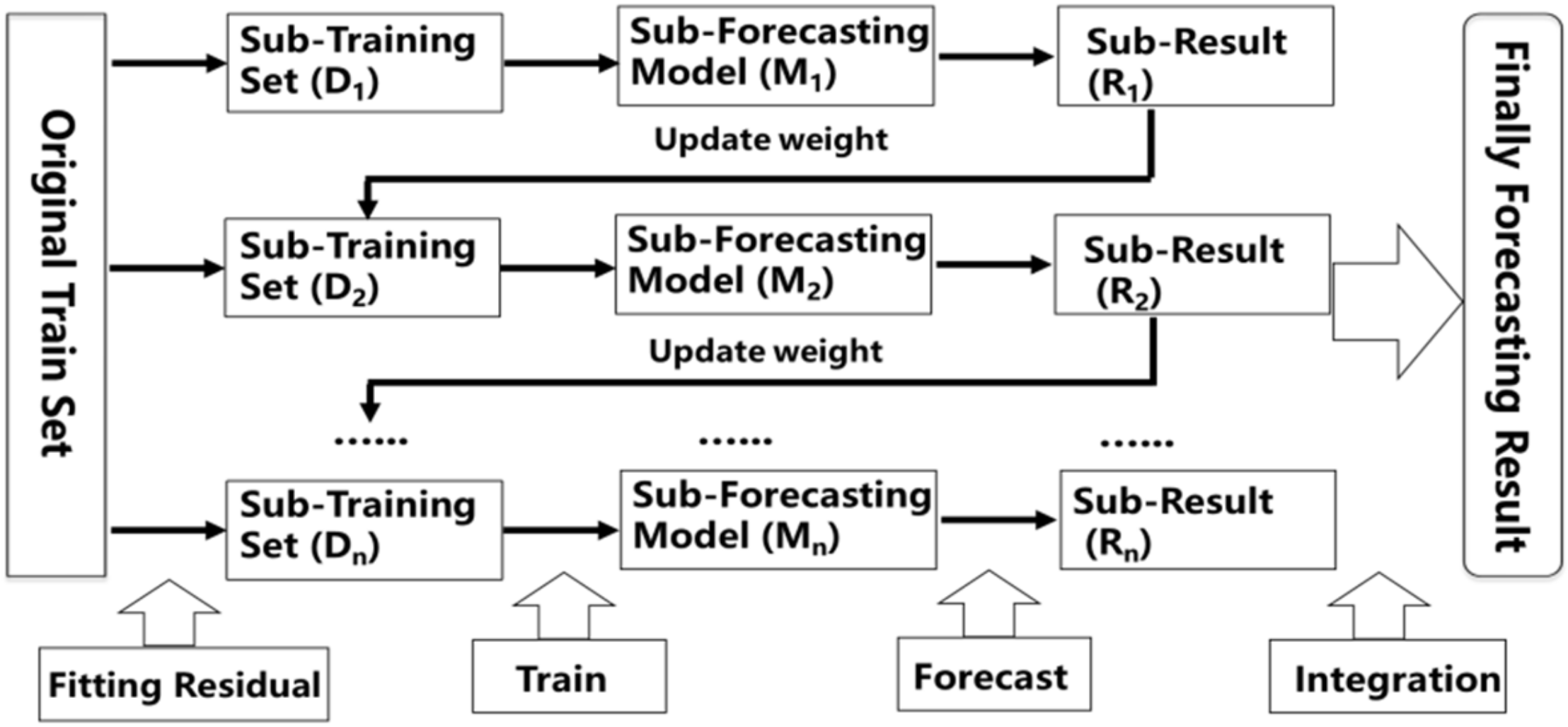
In this paper, we summarize the Filter, Wrapper, and Embedded theories from FS based on ML and apply Partial Mutual Information (PMI), Recursive Feature Elimination (RFE), Classification and Regression Tree (CART) as the typical algorithms of the above three theories to select forecast factors suitable for medium and long-term runoff forecast. In the meanwhile, we also summarize the Bagging and Boosting frameworks from EL based-on ML and apply RF and XGB are the representative models of the above two frameworks to realize the forecast which lead time for the next month, next quarter, and next year, respectively. Besides, precision evaluation indexes are employed to compare and analyze forecast results of different schemes and models, which contain Relative Error (RE), Mean Value of Absolute Relative Error (MAPE), NASH Efficiency Coefficient (NSE), and Relative Root Mean Square Error (RRMSE). This paper is structured as follows. The theories of FS and EL are described in
Section 2. A case study that contains catchment and research results is detailed in
Section 3. The study is summarized and concluded in
Section 4.
3. Case Study
3.1. Study Area
In the paper, we apply the proposed methodology to the Three Gorges Reservoir which is located in the Yangtze River Basin. The Yangtze River is the longest and most abundant river in China, with a total length of 6300 km. As the third longest river in the world, its total amount of water resources is 961.6 billion cubic meters, accounting for about 36% of the total river runoff in the country, 20 times that of the Yellow River. Above Yichang is the upper reaches of the Yangtze River, with a length of 4504 km and a basin area of one million square meters. Yichang to Hukou is the middle reaches, with a length of 955 km and a basin area of 0.68 million square meters. Below Hukou is the downstream, with a length of 938 km and a basin area of 0.12 million square meters. The Three Gorges Reservoir, located in Yichang City, is the largest water conservancy project in China and has a series of functions such as flood control, irrigation, shipping, and power generation. Its control basin accounts for about 60% of the Yangtze River basin, with a total area of 1084 square meters, a total capacity of 30.3 billion cubic meters and an average flow of 15,000 cubic meters per second for many years [
58,
59].
3.2. Predictors
The forecast factors are based on 130 remote-related climate indexes provided by the National Climate Center (China) (
https://cmdp.ncc-cma.net/Monitoring/cn_index_130.php accessed on 4 April 2021). Climate indexes contain three parts. The first part includes 88 atmospheric circulation indexes such as Subtropical High, Polar Vortex, Subtropical High Ridge, Zonal/Meridional Circulation, Pattern Index, Wind Index, etc. All the atmospheric circulation indexes have an exact location, strength and range. The second part is about 26 sea surface temperature indexes which include NINO 1 + 2 SSTA Index, NINO 3.4 SSTA Index, Indian Ocean Basin-Wide Index, South Indian Ocean Dipole Index, etc. The third part includes 16 other indexes such as Cold Air Activity Index, Total Sunspot Number Index, Southern Oscillation Index, etc. The detail of 130 remote-related climate indexes can be found on the website of National Climate Center (China).
As mentioned in
Section 2.1, schemes named A, B, C as three kinds forecast factors, which are used as the representatives of theory of Filter, Wrapper and Embedded. Due to the space limitation in this paper, only the predictors of January in monthly forecast at Three Gorges Reservoir are shown as an example. The predictors are as follows in the
Table 1. Since the factors are all previous year, the first number means the specific month. For example, 5_Western Pacific Subtropical High Intensity Index represents the value of this climate index in May last year.
3.3. Precision Evaluation Indexes
The model accuracy analysis is based on six performance indexes that have been widely used to evaluate the good-ness-of-fit of hydrologic models. Although there are other hydrological evaluation indexes, we intend to use Square of Correlation Coefficient (R2), Relative Root Mean Square Error (RRMSE), Relative Error (RE), Mean Absolute Percentage Error (MAPE), Nash-Sutcliffe Coefficient of Efficiency (NSE) and Qualification Rate (QR). In the following description, , , and are observed values, simulated values, mean of observed sequences and mean of simulated sequences, respectively. The values of n and N are the qualified length and total length of data set, respectively.
- (1)
Square of correlation coefficient (R2)
R
2 is one of the most employed criteria to evaluate model efficiency. Its range between −1 and 1 (perfect fit) and it is defined as:
- (2)
Relative Root Mean Square Error (RRMSE)
RRMSE is based on RMSE which is not suitable for comparing different magnitudes of streamflow, i.e., RRMSE which ranges from −1 and 1 shows a good performance to compare runoff sequences in different river basins. RRMSE is calculated as [
60]:
- (3)
Relative Error (RE) and Mean Absolute Percentage Error (MAPE)
RE and MAPE are conventional criteria to show the results in each data point. There are given by:
- (4)
Nash-Sutcliffe Coefficient of Efficiency (NSE)
The
NSE is one of the best performance metrics for reflecting the overall fit of a hydrograph. It varies from −∞ and 1 (perfect fit). If the
NSE value between 0 and 1, it means an acceptable model performance. If
NSE value is lower than 0, it indicates that mean value of the series is a better estimation than the constructed model.
NSE is defined as [
61]:
3.4. Monthly Forecast
Python is adopted as the programming platform this time, including open-source databases Numpy, Pandas, Scikit-Learn, etc. The runoff sequences are calibrated over the 37-year period 1965–2001 and validated over the 15-year period 2002–2016. The parameters of RF and XGB models in different scales are determined by the fitting effect in calibration. In order to verify the adaptability and accuracy of the three predictors selection methods and the two types of machine learning for medium and long-term forecast models in different timescales, the forecast lead time focus on one month, one quarter and one year, respectively.
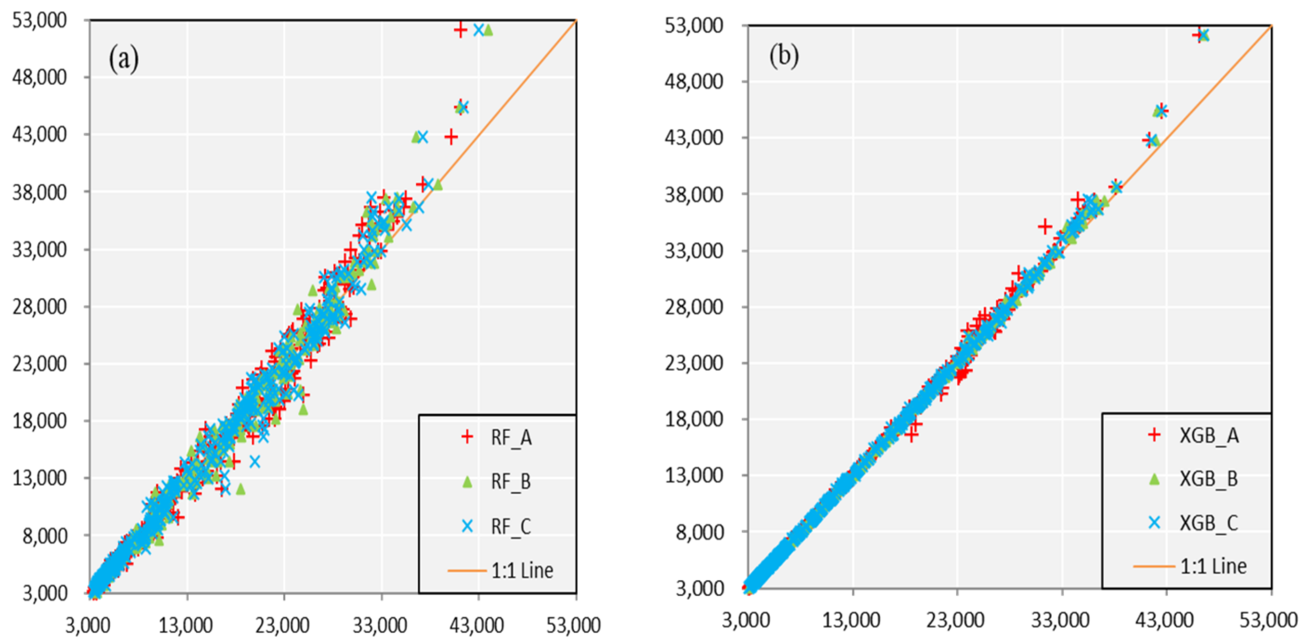
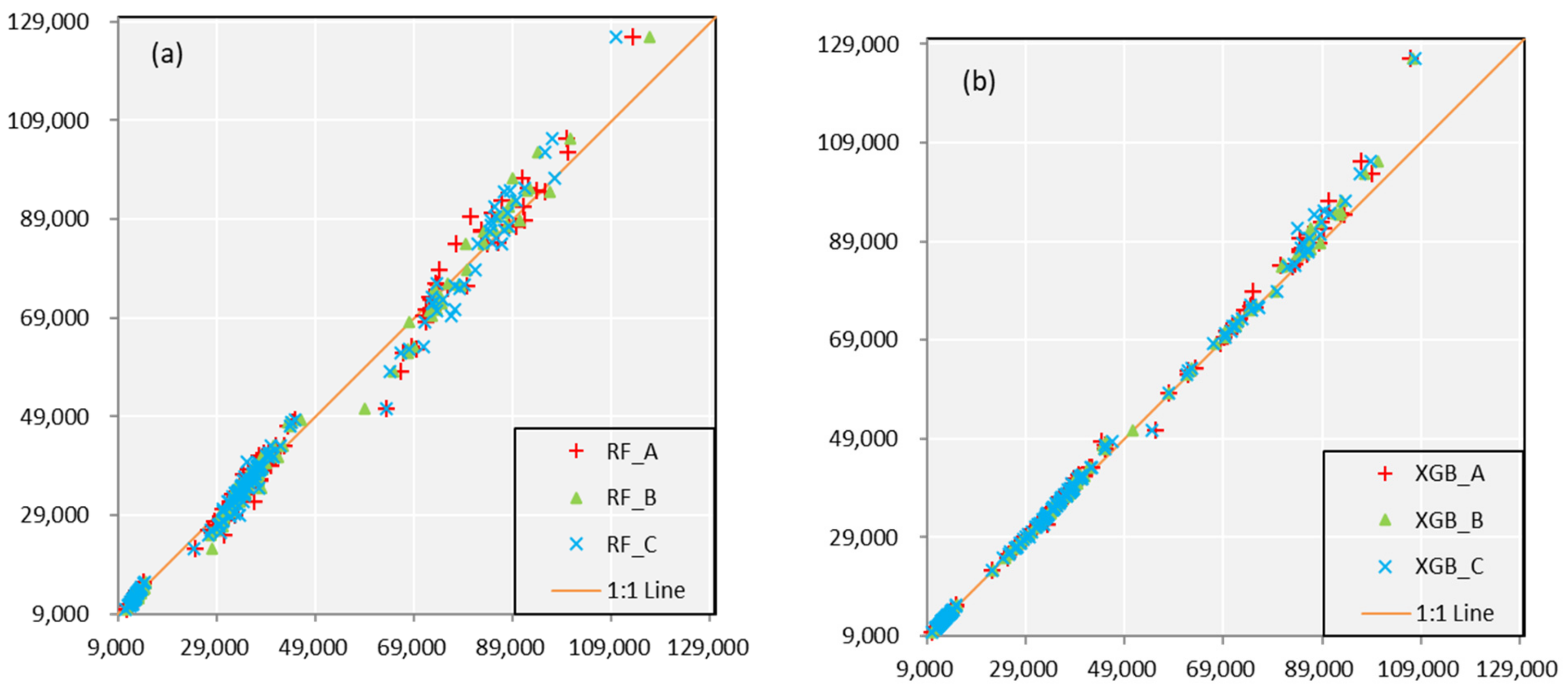
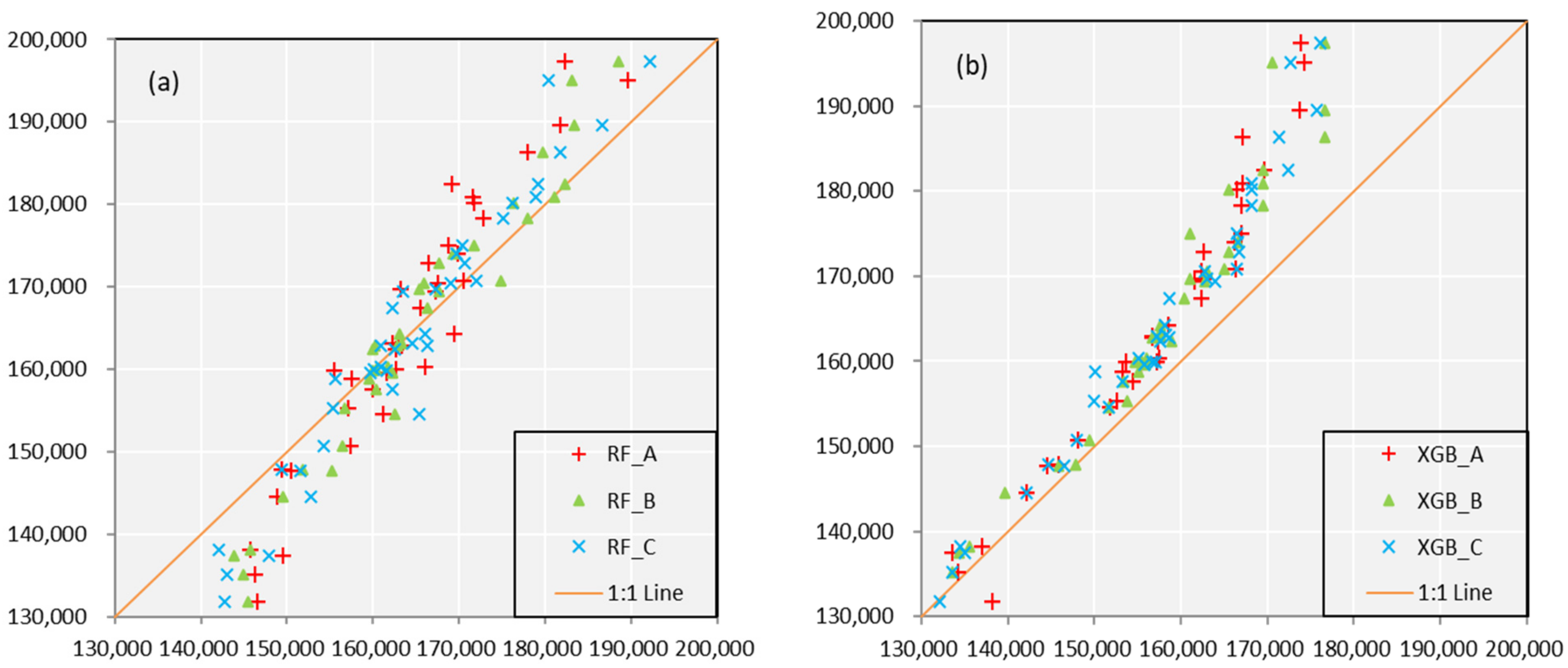
As shown in
Figure 3, for the situation of different models with same predictors’ schemes, the accuracy in calibration of XGB is better than that of RF. Scatters in XGB are much closer the 1:1 line which means a perfect fitness. In the meanwhile, all the values on the scatterplots are evenly located at both sides of orange line, show little indication of system deviation. For another situation of same models with different predictors’ schemes, it shows a similar accuracy and adaptation. It is difficult to compare the performance of the Scheme A, Scheme B, and Scheme C from the graphs. The precision evaluation indexes are shown in the following
Table 2 which contains the specific values towards three schemes and two monthly forecast models. Data in the table further verify the above conclusions.
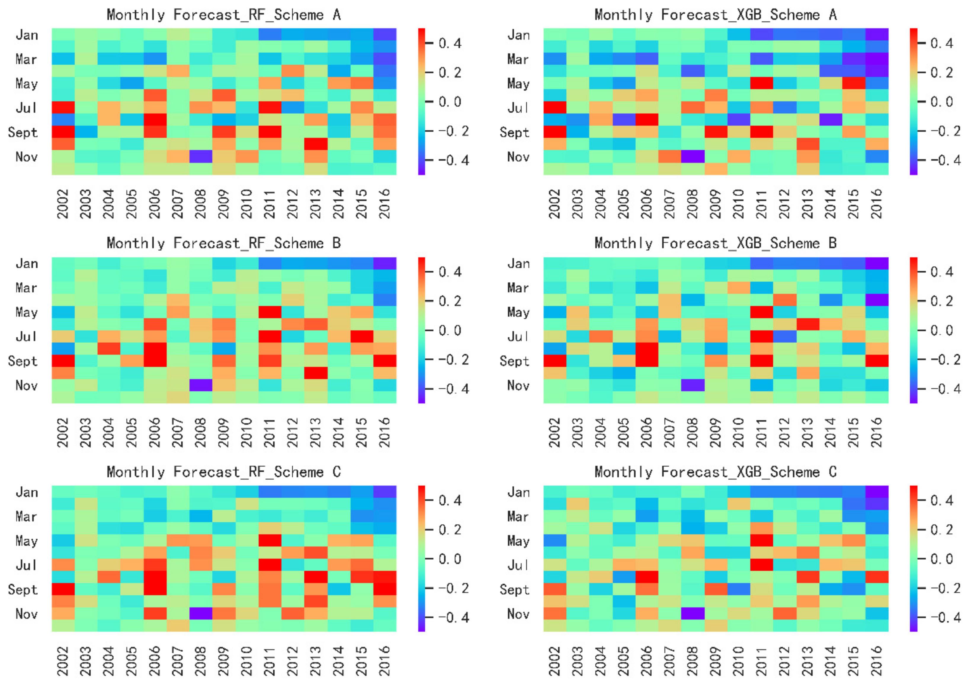
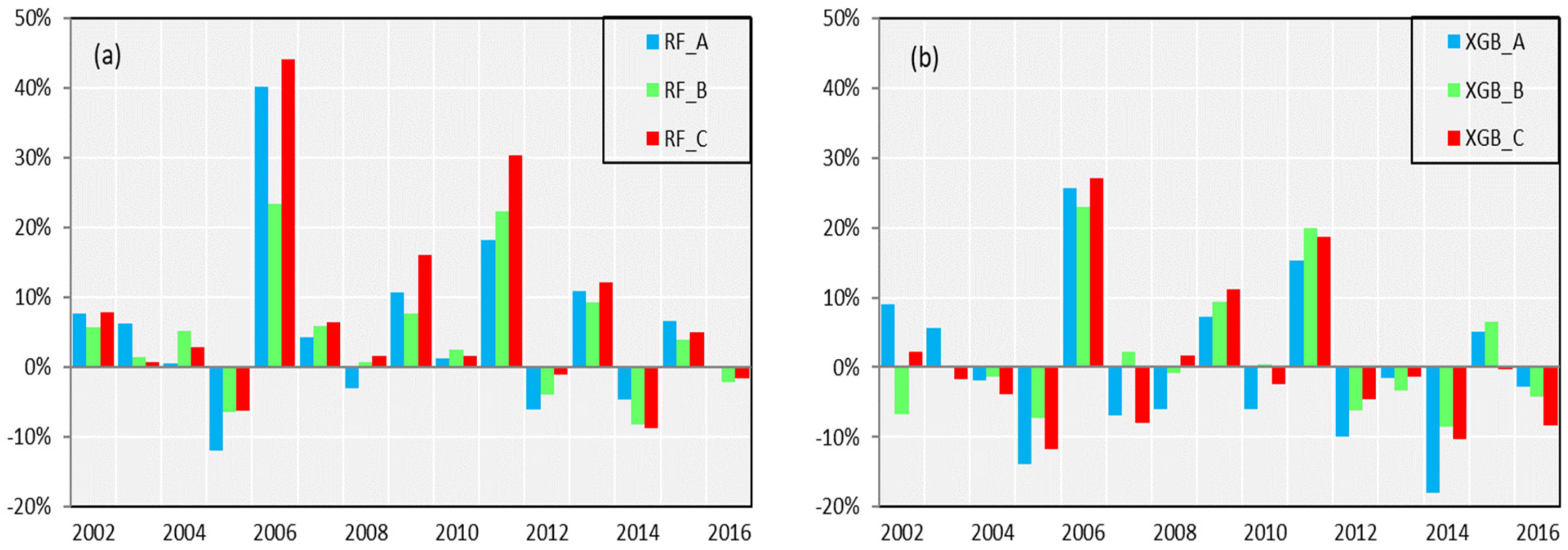
In the validation period, the specific RE is shown as
Figure 4 and
Table 3. For the heatmaps, red indicates that the predicted is greater than the observed value, and blue indicates that the predicted is less than the measured value. According to the value of RE, set the legend to +50% at the maximum and −50% at the minimum and the darker the color, the greater the absolute value of the RE. In the horizontal direction of
Figure 4, the left and right is RF and XGB model. In the vertical direction, there are Scheme A, B, and C, respectively.
Generally speaking, the forecasts of Jan and July to Oct are much worse than other months.
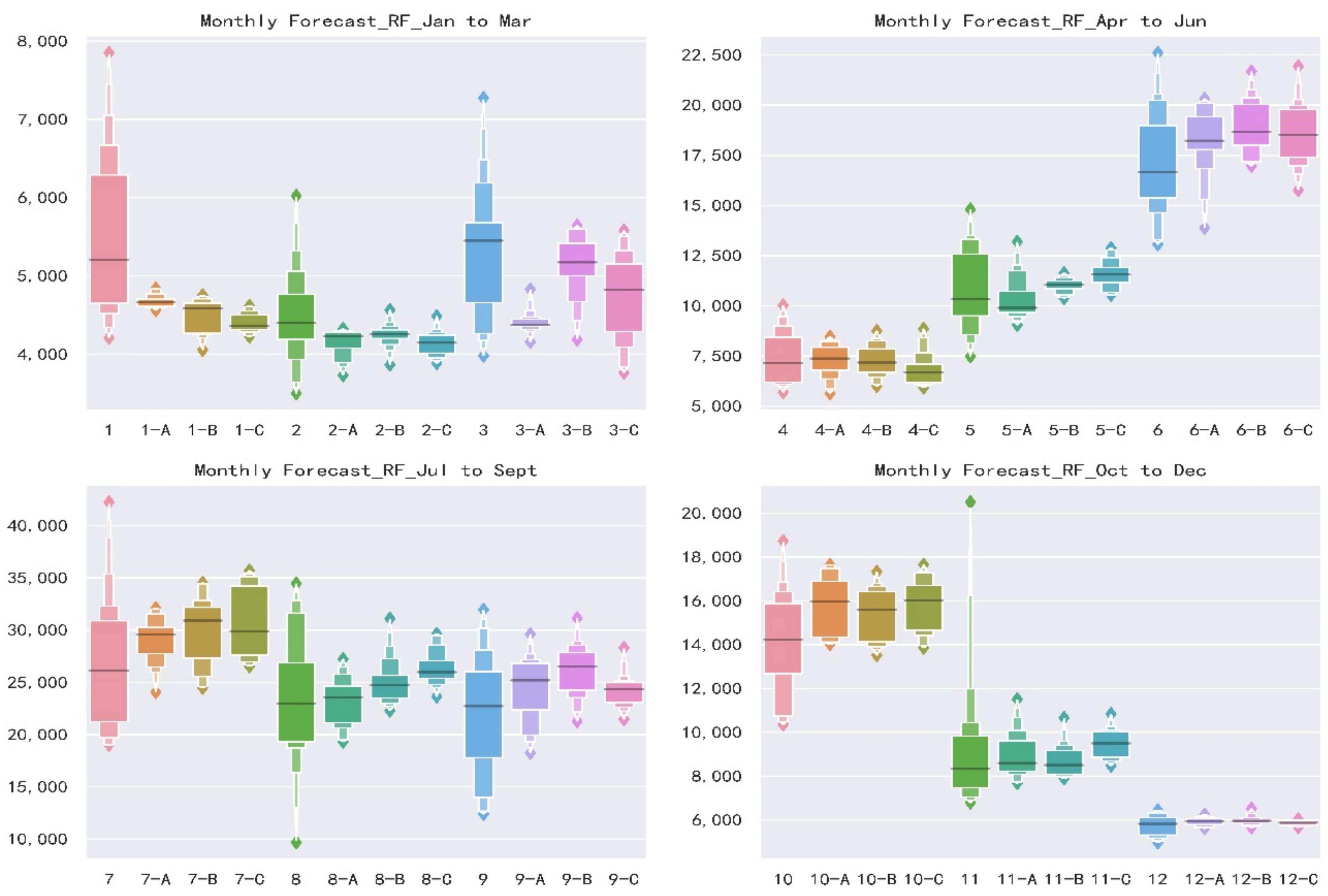
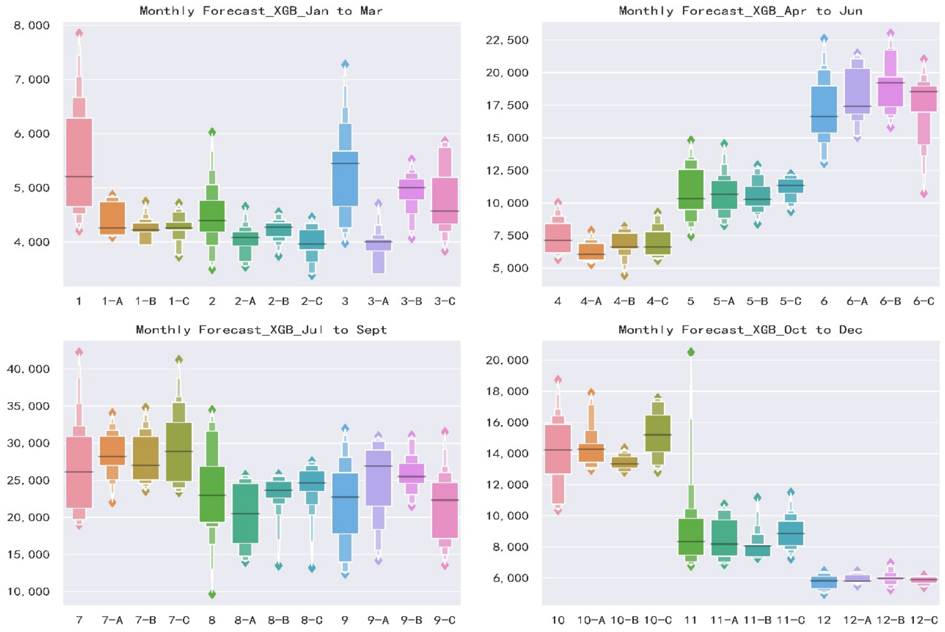
Figure 5 presents an enhanced boxplot named letter-value plot [
62]. Standard boxplots consist of the outliers, maximum, upper quartile, median, lower quartile, minimum and outliers from top to bottom. Boxplots are useful to illustrate the rough information about the distribution of the variables but do not take advantage of precise estimates of tail behavior, i.e., the specific data distribution cannot be displayed. As for letter-value plot, in addition to drawing the original quartiles, it continues to draw 8th, 16th, 32nd, etc., and the width and color depth of each box correspond to the corresponding sample size. Based on letter-value plots, we could tell the concentration and dispersion of monthly runoff, which not only shows the position of the data quintiles, but also shows the probability density of any position. As the runoff of Jan, July to Oct shown in
Figure 5, the distributions of observed values are extremely scattered, and the annual differences are large. Transversely, the distributions are relatively uniform, and the repeat abilities are low. This feature of runoff increases the difficulty of forecast.
In general, the horizontal comparison shows that XGB model has a slightly better forecast result than RF model under the same forecast factors. At the same time, the vertical comparison shows that for the same forecast model, Scheme B has the highest accuracy, and Schemes A and C are similar.
3.5. Seasonal Forecast
When forecasting the runoff in the next quarter, 130 remote-related climate indexes with an advance of one year are still used as forecast factors, and the total runoff values of each quarters are used as forecast targets, with the calibration and validation period the same as monthly forecast.
Figure 6 and
Table 4 show the forecast results of the two models in calibration, and similar conclusions which according to
Figure 3 and
Table 2 can be obtained.
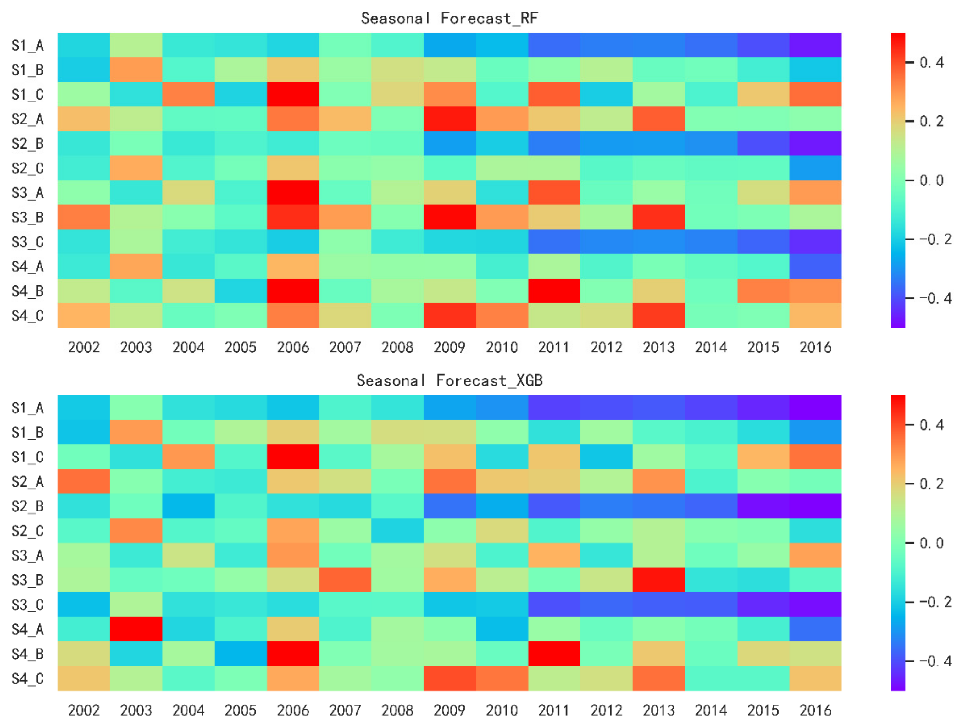
As can be seen from
Figure 7, in general, the forecast results of the validation period are similar for the two models with the same forecast factor scheme. Except for the poor forecast results in 2006, 2009 and the first quarter combined Scheme A, the second quarter’s combined Scheme B and the third quarter combined Scheme C from 2010 to 2016, the results are still acceptable.
Table 5 shows similar results to those shown in
Table 3, except for further demonstration of the above results, the results of Scheme B are the best, slightly better than those of Scheme A and C, and the latter two results are parallel.
3.6. Annual Forecast
When forecasting the runoff for the next year, 130 remote-related climate indexes with an advance of one year are still used as forecast factors, and the total runoff values of each years are used as forecast targets, with the calibration and validation period the same as monthly forecast. Because the data sequence is short, only the MAPE is used to evaluate the forecast results. Similar to the previous description, scatterplots are employed to illustrate the accuracy shown in
Figure 8 and
Table 6. There still displays a closely phenomenon that XGB is better than RF model in calibration. It is worth noting that, for the annual forecast, the RF shows that the lower observation contributes under-estimates, and the higher observation contributes the over-estimates. As for XGB, most cases are overestimated, and with the increase of observed values, the overestimation phenomenon becomes more obvious. One possible reason is that the annual runoff varies greatly from year to year. In the period of model building, some extreme values significantly affect the modelling process, resulting in overestimation/underestimation on the whole. We will pay attention to this in the follow-up research.
Figure 9 and
Table 6 demonstrates a specific RE for three schemes in each year. For the case of RF/XGB models under different forecast factors, Scheme B represents the best forecast skill. For the situation of three schemes under different models, XGB shows a higher accuracy and stability than RF model both in validation and calibration.
4. Conclusions
For the medium and long-term runoff forecast on the monthly-seasonal-annual scale, the difficulty and emphasis include two parts. The first is to select accurate and stable forecast factors with certain physical causes, and the second is to build forecast models with clear theory and good forecast.
In this paper, we summarize three typical methods of Feature Selection theory based on Machine Learning in the selection of forecast factors and employ PMI, RFE, and CART as typical algorithms of Filter, Wrapper, and Embedded, respectively, to obtain three sets of forecast factor schemes. In the meanwhile, we summarize two typical theories of Ensemble Learning based on Machine Learning, and selected RF and XGB as typical models for Bagging and Boosting to simulate and forecast runoff sequences. The above forecasting frameworks are applied to the Three Gorges Reservoir in the Yangtze River Basin to realize monthly-seasonal-annual runoff forecast. Through the forecast results in the periods of calibration and validation, the following conclusions can be obtained:
- (1)
For three schemes, Scheme B shows the best forecast skills, highest accuracy and stability when comparing the same forecast lead time and models. Scheme A and Scheme C have similar results and are slightly inferior to Scheme B. It illustrates that taking the forecast performance of the learners to be used as the evaluation criterion for the FS is an effective and efficient approach.
- (2)
For two models, XGB shows a better forecast result than RF model during the calibration period when comparing the same forecast lead time and predictors. Furthermore, in the validation period, XGB also shows a smaller forecast error if only taking Scheme B as a comparison. This is not to say that XGB is a better model than RF for two reasons. Firstly, it requires more basin data to verify whether there are differences in forecasting skill. Secondly, among some forecast factor schemes, RF displays a better performance. Therefore, the Ensemble Learning algorithms based on two different frameworks are suitable for medium and long-term runoff forecast.
- (3)
For three different forecast lead time, it shows an interesting phenomenon. According to the most commonly used MAPE index, the annual runoff forecasting error is the smallest. MAPE is 8.34% and 7.11% in RF and XGB model, respectively, while the monthly and seasonal runoff forecast results are similar, and MAPE floats around 16%. This demonstrates that with the increase of the runoff magnitudes, the instability and non-uniformity of the distribution of the extreme value series are reduced, and the accuracy and stability of forecast are improved.


