An Equivalent Pipe Network Modeling Approach for Characterizing Fluid Flow through Three-Dimensional Fracture Networks: Verification and Applications

Abstract

The equivalent pipe network (EPN) model is an effective way to model fluid flow in large-scale fractured rock masses with a complex fracture network due to its straightforwardness and computational efficiency. This study presents the EPN model for characterizing fluid flow through three-dimensional fracture networks using the Monte-Carlo method. The EPN model is extracted from an original three-dimensional discrete fracture network (DFN) model and is used to simulate the fluid flow processes. The validity of the proposed EPN modeling approach is verified via the comparisons of permeability (k) with analytical solutions and simulation results reported in the literature. The results show that the numerically calculated k using EPN models agrees well with the analytical values of simplified DFN models and the simulation results of complex DFN models. The k increases following an exponential function with the increment of mean length of exponentially distributed fractures (u), which is strongly correlated with fracture density (P₃₂) and average intersection length (L_i). The P₃₂ increases in an exponential way with the increment of u. The L_i increases as u increases, following a power-law function. The increment of u leads to the increment of a number of long fractures in three-dimensional DFN models. A larger u results in a denser fracture network and a stronger conductivity when the number and length distribution range of fractures remain the same. The representative elementary volumes (REVs) of three-dimensional DFN models with u = 9 m and P₃₂ = 0.4 m²/m³ are determined as 2.36 × 10⁴ m³, 9.16 × 10³ m^3, and 1.26 × 10⁴ m³ in 3 flow directions, respectively.

1. Introduction

In fractured rock masses with low matrix permeability, such as tight sedimentary and crystalline rocks, the fractures provide main flow paths for fluids [1,2,3,4,5,6,7,8,9,10,11]. The transport and fluid flow properties through such fractured rock masses are dominated by the connectivity of fracture networks that are determined by a variety of statistical geometrical characteristics. Owing to the difficulties of characterization and modeling of fracture networks and computational limitations [1,12,13,14,15,16,17,18,19], the fluid flow simulations through fractured rock masses are commonly simplified to two-dimensional (2D) problems, which underestimates the permeability of real three-dimensional (3D) fracture networks [9,20,21,22,23]. It is thus important to characterize and model fluid flow to assess the impact of statistic geometrical characteristics on seepage properties of fractured rock masses using 3D models [24,25].

The investigations of geometrical characteristics of fractures spread through an extensive range of scales from core to satellite imagery and aerial photograph scales [4,26]. However, a large number of fractures are hidden in the interior of the rock masses, and it is difficult to directly measure the fracture morphologies. The fracture morphology is diverse depending on rock types and surrounding environments. Since the 1970s, the scaling attributes of fracture networks have received increasing attention, motivated by the promise of statistical prediction that scaling laws offer. The exponential law has been used to describe the size distribution of discontinuities in rock masses [27,28,29,30,31,32,33,34,35]. Numerical simulation results from Cowie et al. show that the exponential distribution of fracture lengths is affected by the early stage of deformations [36]. Due to the difficulties of directly performing an accurate measurement of geometrical characterizations of large-scale natural fracture systems, the discrete fracture network (DFN) modeling approach has been adopted [37]. The DFN modeling approach commonly simplifies the fractures as straight-line segments in 2D and convex polygons or discs in 3D [38]. The two idealizations are very simplified, but they are able to model any sort of complexity in the shape of fractures [37,39,40]. Generally, transforming the DFN model into an equivalent pipe network (EPN) model, which has approximately equivalent hydraulic properties and connectivity with planar fractures, is an effective method for analyzing the connectivity and percolation characteristics of a disc fracture network [41,42,43,44,45].

In a former study, the authors developed an EPN approach, in which the flow occurs through bonds joining the center of each disk to the center of intersections between two adjacent fractures [41]. The authors also simulated the fluid flow through the petroleum field by introducing the networks of fluid domains and pipes, which is similar to the method proposed by Cacas et al. [41,46]. They developed three-channel geometries for flow and transport within the fractures, including tubular flow channels, parallel plate channels with a constant width, and parallel plate channels with widths equaling the fracture intersection line length. The recent study transformed the 3D DFN model to an EPN model with an equivalent hydraulic conductivity of fractures and demonstrated that the hydraulic behaviors of pipe networks could be equivalent to that of polygonal-element DFN models [20]. Moreover, the authors proposed a proper EPN model that can represent the DFN model generated by statistical geometrical parameters, and the validity was verified by comparisons with other methods. Open-source software for establishing EPN models, Alghalandis Discrete Fracture Network Engineering (ADFNE) (Alghalandis Computing, Toronto, Canada), has been developed to characterize fluid flow, intersection properties, and connectivity by extracting backbone structures consisting of pipes with a circular section [44]. Furthermore, the DFN model established by geological survey data of Xinchang high-level radioactive waste (HLW) is equivalent to a pipe network model to estimate the hydraulic properties of rock masses and corresponding representative elementary volume (REV) size [45]. The EPN model is an effective way to simulate fluid flow in a large-scale complex fracture network due to its straightforwardness and computational efficiency. However, the effectiveness of the EPN model and the impact of statistical geometrical characteristics of fractured geometrical elements on hydraulic characteristics of fractured rock masses by the EPN model is rarely discussed in previous works. Due to the scale-dependent hydraulic properties of fractured rock masses, the REV size is necessarily determined by calculating the permeability (k) of DFN models (

Table A1. The list of symbols.

Symbol	Meaning and Unit
Q	The total flow rate through single fracture or fracture network (m3/s)
g	The gravity acceleration (m/s2)
v	The kinematic viscosity of the fluid (m2/s)
a	Fracture aperture (m)
w	The section width (m)
J	Hydraulic gradient
Hin	The water head applied on the inlet boundary (m)
Hout	The water head applied on the outlet boundary (m)
Ldis	The distance between the opposite boundaries of fracture network models (m)
Cij	The equivalent conductance of the pipe between node i and node j (m2/s)
Lij	The length of the pipe between node i and node j (m)
Qij	The flow rate through the pipe between node i and node j (m3/s)
Hi	The water head of node i (m)
Hj	The water head of node j (m)
△H	Water head difference between adjacent nodes (m)
k	Equivalent permeability (m2)
ks	The equivalent permeability of the equivalent pipe network model (m2)
kt	The equivalent permeability of the simplified discrete fracture network model (m2)
ε	The relative error between kt and ks (%)
u	The average value of fracture length (m)
Li	The average value of intersection length between fractures (m)
P32	The total area of fracture surface per unit volume (m2/m3)

).

The present study simplifies the DFN model to the EPN model to assess the evolutions of hydraulic characteristics of fractured rock masses, in which the fracture length distribution follows the exponential function. The validity of the EPN model was verified by comparing the simulation results of the EPN model with the analytical results of simplified DFN models and simulation results of complex DFN models reported in the literature. The k is calculated by applying different hydraulic boundary conditions, and the REV sizes in different flow directions are determined according to the variations in K for the models with different sizes.

2. Generation of DFN and EPN Models

Efficient 3D DFN models were generated based on the statistical geometrical characteristics of fracture networks. The fractures distributed within the model were simulated using the Monte-Carlo method. The DFN model was simplified to the EPN model by treating the fractures as pipes.

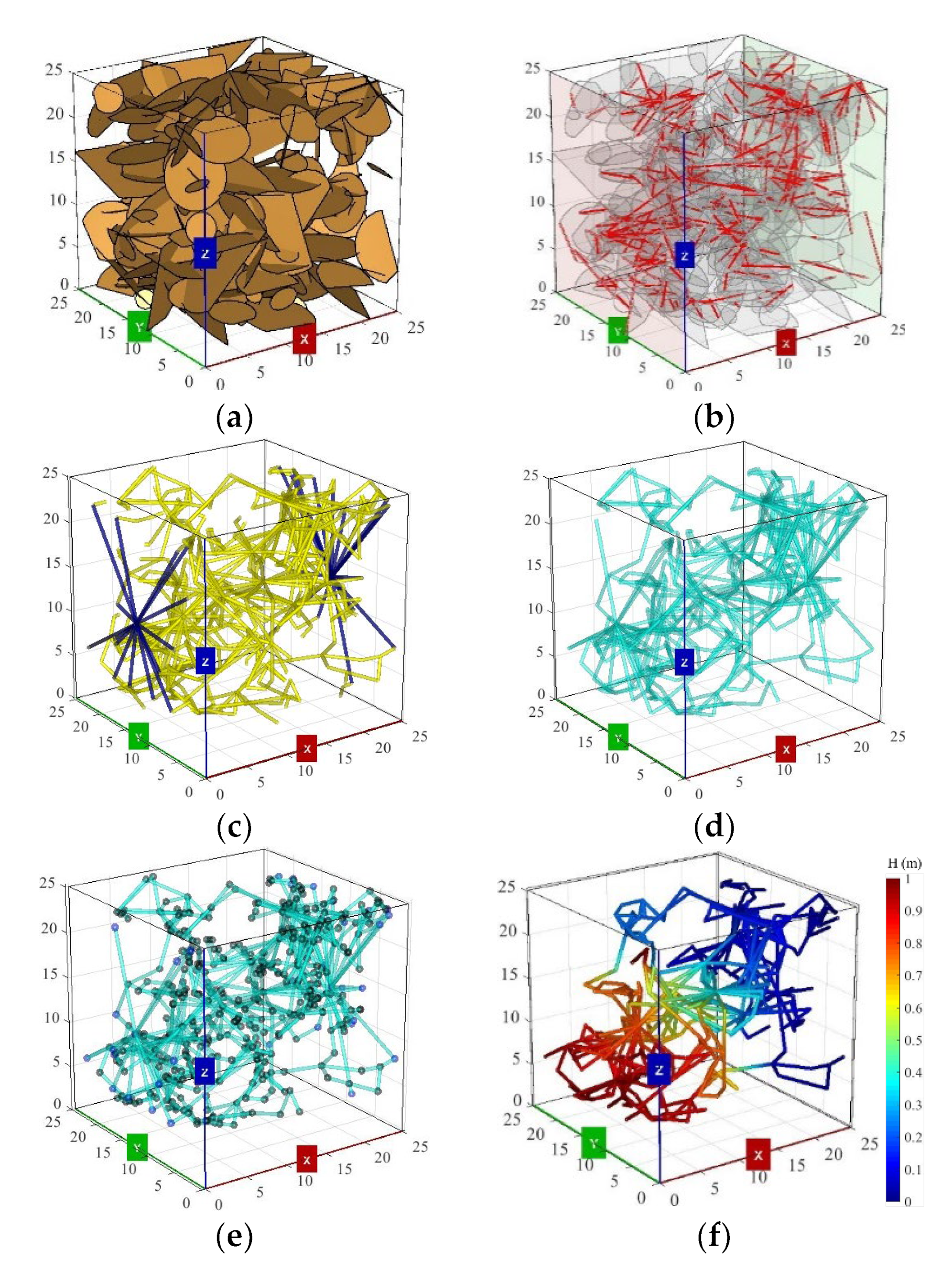
2.1. Generation of 3D DFN Models

A fracture can be characterized by a circle and/or ellipse based on field investigations and trace data evaluations. In the present study, the fractures are assumed to be circle discs embedded in an impermeable rock matrix. First, the exponential distribution of fracture lengths is assumed to generate fracture lengths. Here, fracture length denotes the diameter of the circles. Then, the fracture discs are located within the model as a connected network that has statistical distributions of dip angle and dip direction. The center point location of fracture discs may follow uniform, Poisson, or other random distributions. Finally, the orientation is assumed to follow Fisher or uniform random distributions.

An example of the DFN model containing 200 fractures is shown in Figure 1a, and the intersections between fractures are presented in Figure 1b with red lines. The side length is 25 m, and the fracture length follows an exponential distribution between 1.25 m and 15 m with a mean value of 7.5 m. The aperture of all fractures is fixed to be a constant of 1 mm. The dip directions of fractures are assumed to follow Fisher distribution in a range of [0, 2π), and the dip angles of fractures are assumed to follow Fisher distribution in the range of [0, π/2).

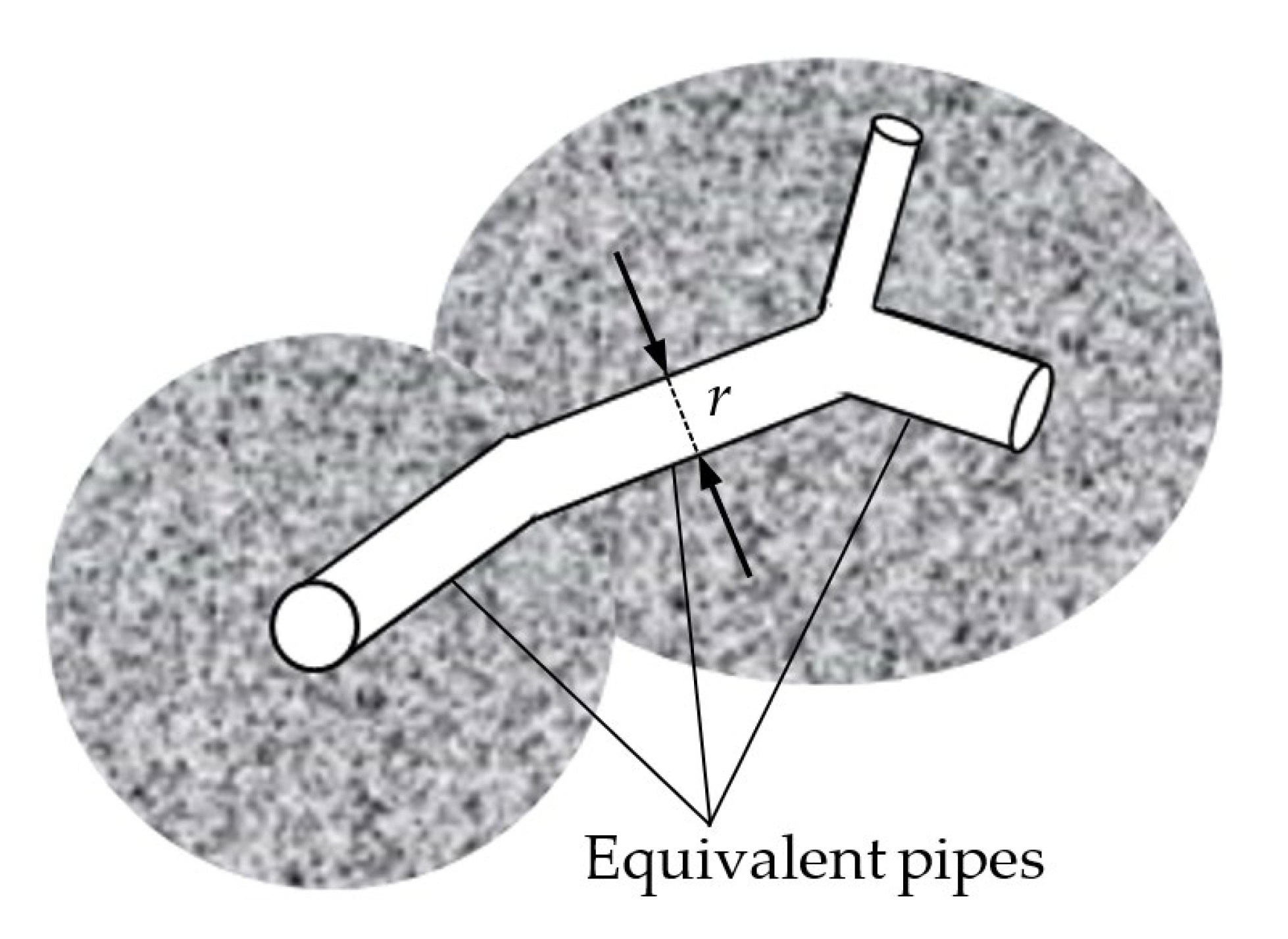
2.2. Generation of 3D EPN Models

A MATLAB (MathWorks, Natick, MA, USA) code is developed to generate the geometrical data of DFN models, which are then simplified to EPN models using an open-source software ADFNE [44]. Figure 1c–f show the pipe structure, backbone structure, nodes and edges, and water head distributions of a fracture network. Here, the fluid is assumed to flow from the yz plane at x = 0 m to the yz plane at x = 25 m with a water head difference of 1 m. The fractures are represented by pipes connecting the disc centroid and the centers of intersections with other fractures, as shown in Figure 2. The isolated and dead-end pipes are eliminated from the framework, as shown in Figure 1c, to promote further evaluations of the pathways. Figure 1e shows the pathways for the presented DFN model, in which boundary (outer) nodes and inner nodes are marked. However, the hydraulic water heads of inner nodes inside the targeted region are unknown and should be solved. A simple technique for modeling fluid flow is proposed by the application of the finite difference method [39]. The basics are well studied and documented. Figure 1g,h show that the fracture length distribution follows an exponential function with the correlation coefficient (R²) larger than 0.96, while the pipe length follows a lognormal distribution with R² > 0.92.

3. Verification of the EPN Model

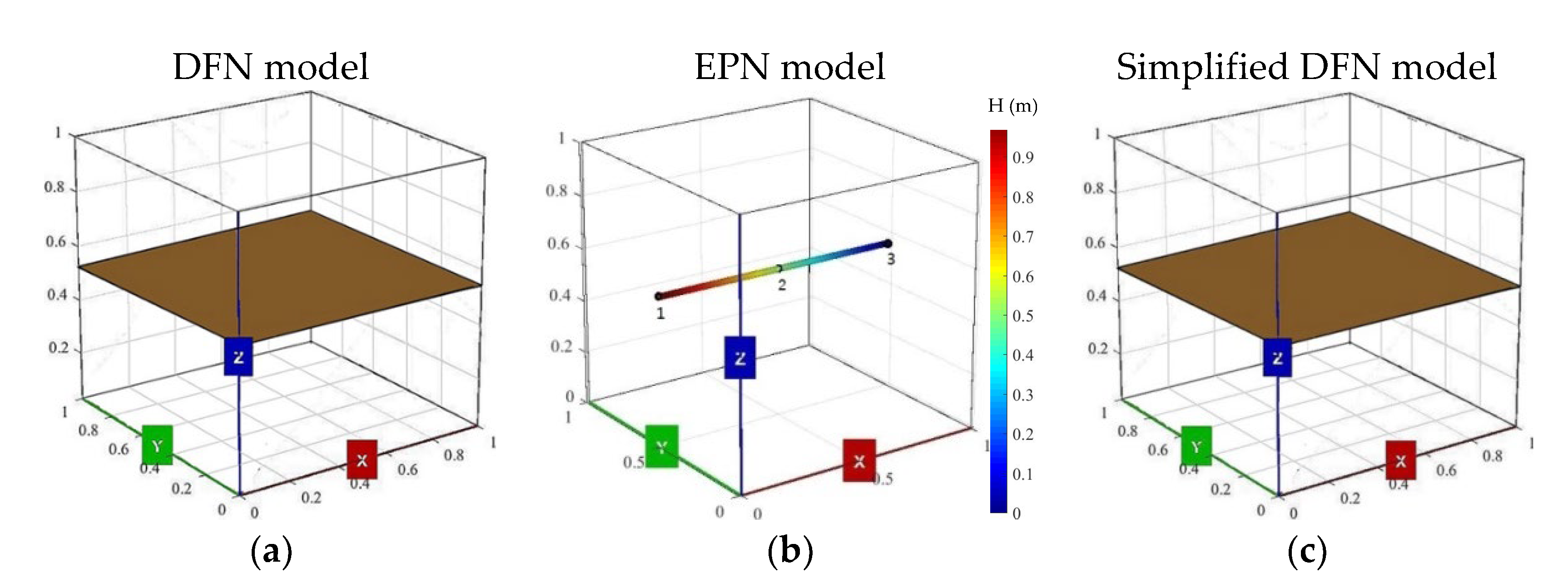
3.1. Validation of the Simple EPN Models

A total of four simple EPN models were established, and fluid flow through them was simulated to verify the validity of the EPN models, in which the fractures are represented by pipes connecting the disc centroid and the centers of intersections with other fractures, as shown in Figure 2. To evaluate the fluid flow in the models, isolated fractures and dead-ends of fractures are deleted in the modeling processes of EPN models and simplified DFN models. Assumptions are made that H_in = 1 m at the yz plane (x = 0 m) and H_out = 0 m at the yz plane (x = 1 m), while the other boundaries are impermeable. Here, H_in and H_out are the inlet and outlet water heads, respectively. A model that only contains a single fracture is shown in Figure 3a with a constant aperture of 1 mm (hereafter, the default value of fracture aperture is equal to 1 mm), and the corresponding EPN model and simplified DFN model are shown in Figure 3b,c respectively. In the simplified DFN model, all income and outcome flow rates to and from an intersection should fully satisfy the mass conservation law. The total flow rate through a single fracture can be calculated according to the cubic law:

$$Q=\frac{g}{v}\frac{a^{3}w}{12}J$$

(1)

where g is the gravity acceleration, v is the kinematic viscosity of the fluid, a is the fracture aperture, w is the section width, J is the hydraulic gradient that equals to the ratio of water head difference at the inlet and outlet boundaries to the length of the model. J can be expressed as:

$$J=\frac{H_{in}-H_{out}}{L_{dis}}$$

(2)

where L_dis is the distance between the opposite boundaries of fracture network models. In Figure 3a, the L_dis and w both equal to 1 m. The Q through the single fracture in Figure 3a can be calculated by:

$$Q=\frac{g}{v}\frac{w{a}^3}{12}J=\frac{g}{v}\frac{w{a}^3}{12}\frac{H_{in}-H_{out}}{L_{dis}}=8.1667\times {10}^{-4} \left({\mathrm{m}}^3·{\mathrm{s}}^{-1}\right)$$

(3)

The k of the DFN model (k_t) in Figure 3c is calculated by:

$$k_t=\frac{\mu Q}{A\rho gJ}=8.3333\times {10}^{-11} \left({\mathrm{m}}^2\right)$$

(4)

The equivalent conductance for each pipe in a steady and laminar flow state is expressed as [39]:

$$C_{ij}=\frac{g·a^3·w}{12·v·L_{ij}}$$

(5)

where C_ij is the equivalent conductance of the pipe between node i and node j, L_ij is the length of the pipe between node i and node j.

The flow rate through a pipe between node i and node j can be calculated as [39]:

$$Q_{ij}=C_{ij}\Delta H=C_{ij}\left(H_i-H_j\right)$$

(6)

where Q_ij is the flow rate between nodes i and j, H_j is the pressure head of node j, H_i is the pressure head of node i.

All income flow to a node and outgoing flow from a node must fully match to ensure mass conservation. The flow rate for node j, which is directly connected to n nodes around it, should follow Equation (7).

$${\displaystyle \sum }_{i=1}^n{Q}_{ij}=0$$

(7)

Substituting Equation (6) into the Equation (7) yields a new governing equation for computing the water head of node j (H_j) as follows:

$$H_j=\frac{{{\displaystyle \sum }}_{i=1}^n{C}_{ij}·H_i}{{{\displaystyle \sum }}_{i=1}^n{C}_{ij}}$$

(8)

The expressions for H_j and C_ij are based on the following assumptions: (1) the rock matrix is incompressible and impermeable, (2) the fluid is incompressible, (3) the two surfaces of fractures are parallel and smooth, and (4) the fluid flow obeys Darcy’s law showing a laminar flow behavior.

The nodes are classified into three types: inlet nodes, inner nodes, and outlet nodes. The fluid flow induced from the water head differences starts at the inlet nodes and reaches the outlet nodes through the inner nodes. The water heads of the nodes on the inlet boundary and outlet boundary are known. The water heads of all inner nodes must be solved by constructing the matrix of unknowns following the above equations. The matrix system (AX = B) is set up to solve X (X = A⁻¹B), in which X is formed by water heads of inner nodes. Assuming that there are a total of m inner nodes, A is m × m coefficient matrix of water heads, X is m × 1 matrix, in which X_j (j = 1 m) is the water head of node j, and B is m × 1 matrix which consists of the constant terms of equations for solving water heads, as follows:

$$\left[\begin{array}{ccc}{A}_{11}& \cdots & A_{1m}\\ ⋮& ⋮& ⋮\\ A_{m1}& \cdots & A_{mm}\end{array}\right]\left\{\begin{array}{l}{H}_1\\ ⋮\\ H_m\end{array}\right\}=\left\{\begin{array}{l}{B}_1\\ ⋮\\ B_m\end{array}\right\}$$

(9)

in which:

$$A_{jk}=\left\{\begin{array}{l}-{\displaystyle {\displaystyle \sum }_{j=1}^n}{C}_{ij} j=k\\ C_{ij} j \mathrm{is} \mathrm{connected} \mathrm{to} k \end{array}\right.$$

(10)

and

$$B_j=\left\{\begin{array}{l}0 j \mathrm{is} \mathrm{inner} \mathrm{node}\\ -C_{ij}{H}_{in} j \mathrm{is} \mathrm{inlet} \mathrm{boundary} \mathrm{node}\\ -C_{ij}{H}_{out} j \mathrm{is} \mathrm{outlet} \mathrm{boundary} \mathrm{node}\end{array}\right.$$

(11)

The flow rate of each pipe can be obtained by Equation (6), and the total flow rate through the EPN model can be obtained by summing the flow rate of each pipe that is connected to the outer nodes. The equivalent permeability of the EPN model (k_s) can be back-calculated according to Darcy’s law, as follows:

$$k_s=\frac{\mu Q}{A\rho gJ}$$

(12)

where μ is the viscosity of the fluid, A is the cross-sectional area, ρ is the density of fluid.

The numbers of inner nodes and outer nodes (corresponding to inflow nodes and outflow nodes, respectively) are 2 and 2 for the example given in Figure 3b. The hydraulic conductivity of each pipe is calculated according to Equation (5), as follows:

$$C_{12}=\frac{g·a^3·w}{12·v·L_{12}}=1.6335\times {10}^{-3} \left({\mathrm{m}}^2·{\mathrm{s}}^{-1}\right)$$

(13)

$$C_{23}=\frac{g·a^3·w}{12·v·L_{23}}=1.6335\times {10}^{-3} \left({\mathrm{m}}^2·{\mathrm{s}}^{-1}\right)$$

(14)

The two water heads at inlet and outlet boundaries are given as follows:

$$H_1=H_{in}=1 \mathrm{m}$$

(15)

$$H_3=H_{out}=0 \mathrm{m}$$

(16)

The H₂ can be calculated by substituting Equations (13)–(16) into Equation (8):

$$H_2=\frac{{{\displaystyle \sum }}_{i=1}^n{C}_{ij}·H_i}{{{\displaystyle \sum }}_{i=1}^n{C}_{ij}}=\frac{C_{12}·H_1+C_{23}·H_3}{C_{12}+C_{23}}=0.5 \mathrm{m}$$

(17)

The flow rate of pipes between node 1 and node 2 (Q₁₂) can be calculated by Equation (6):

$$Q_{12}=C_{12}\Delta H=C_{12}\left(H_1-H_2\right)=8.1675\times {10}^{-4} \left({\mathrm{m}}^3·{\mathrm{s}}^{-1}\right)$$

(18)

The flow through each pipe is equal, as shown in Figure 3b:

$$Q_{12}=Q_{23}=8.1675\times {10}^{-4} \left({\mathrm{m}}^3·{\mathrm{s}}^{-1}\right)$$

(19)

The equivalent permeability of the EPN model (k_s) is calculated as:

$$k_s=\frac{\mu Q}{A\rho gJ}=8.3342\times {10}^{-11} \left({\mathrm{m}}^2\right)$$

(20)

The k_t calculated in Equation (4) agrees well with the simulation result of k_s (see Equation (20)) for DFN model that contains a single fracture. The relative error (ε) between k_t and k_s equals 0.01020%, which is defined as:

ε = | k_t-k_s | / k_t

(21)

Another DFN model contains 2 intersecting fractures, in which the dip angles are 45° and 135°, respectively, as shown in Figure 3d. The corresponding EPN model and simplified DFN model are presented in Figure 3e,f. The total flow rate through a single fracture can be calculated according to Equations (1) and (2), in which the water head of the intersection is assumed to be H, the flow rates (Q₁ and Q₂) through the two simplified fractures in Figure 3f are expressed as:

$$Q_1=\frac{g}{v}\frac{w{a}^3}{12}\frac{H_1-H}{L_1}$$

(22)

$$Q_2=\frac{g}{v}\frac{w{a}^3}{12}\frac{H-H_2}{L_2}$$

(23)

The flow rate through the two simplified fractures is equal as:

$$Q_1=Q_2$$

(24)

Substituting Equations (22) and (23) into Equation (24) results in the solution of H, as follows:

$$H=0.3133 \left(\mathrm{m}\right)$$

(25)

The flow rate through the simplified DFN model is expressed as:

$$Q=Q_1=Q_2=5.7748\times {10}^{-4} \left({\mathrm{m}}^3·{\mathrm{s}}^{-1}\right)$$

(26)

The k of the simplified DFN model in Figure 3f is calculated:

$$k_t=\frac{\mu Q}{A\rho gJ}=5.8927\times {10}^{-11} ({\mathrm{m}}^2)$$

(27)

The numbers of inner nodes and outer nodes (inflow nodes and outflow nodes) are 3 and 2 for the model in Figure 3e, in which boundary conditions follow the above assumptions. The hydraulic conductivity of each pipe is calculated according to Equation (5), as follows:

$$C_{12}=\frac{g·a^3·w}{12·v·L_{12}}=1.1847\times {10}^{-3} \left({\mathrm{m}}^2·{\mathrm{s}}^{-1}\right)$$

(28)

$$C_{23}=\frac{g·a^3·w}{12·v·L_{23}}=2.9028\times {10}^{-3} \left({\mathrm{m}}^2·{\mathrm{s}}^{-1}\right)$$

(29)

$$C_{34}=\frac{g·a^3·w}{12·v·L_{34}}=4.7187\times {10}^{-2} \left({\mathrm{m}}^2·{\mathrm{s}}^{-1}\right)$$

(30)

$$C_{45}=\frac{g·a^3·w}{12·v·L_{45}}=1.9198\times {10}^{-3} \left({\mathrm{m}}^2·{\mathrm{s}}^{-1}\right)$$

(31)

The two water heads (H₁ and H₅) at inlet and outlet boundaries are given as follows:

$$H_1=H_{in}=1 \mathrm{m}$$

(32)

$$H_5=H_{out}=0 \mathrm{m}$$

(33)

Substituting the above Equations (28)–(33) into Equation (8) yields the expressions of the water heads of nodes 2, 3, 4 (H₂, H₃ and H₄) as follows:

$$H_2=\frac{{{\displaystyle \sum }}_{i=1}^n{C}_{ij}·H_i}{{{\displaystyle \sum }}_{i=1}^n{C}_{ij}}=\frac{C_{12}·H_1+C_{23}·H_3}{C_{12}+C_{23}}$$

(34)

$$H_3=\frac{{{\displaystyle \sum }}_{i=1}^n{C}_{ij}·H_i}{{{\displaystyle \sum }}_{i=1}^n{C}_{ij}}=\frac{C_{34}·H_4+C_{23}·H_2}{C_{34}+C_{23}}$$

(35)

$$H_4=\frac{{{\displaystyle \sum }}_{i=1}^n{C}_{ij}·H_i}{{{\displaystyle \sum }}_{i=1}^n{C}_{ij}}=\frac{C_{34}·H_3+C_{45}·H_5}{C_{34}+C_{45}}$$

(36)

Equations (34)–(36) can be rewritten as:

$$-(C_{12}+C_{23})·H_2+C_{23}·H_3=-C_{12}·H_1$$

(37)

$${\mathrm{C}}_{23}·{\mathrm{H}}_2-({\mathrm{C}}_{34}+{\mathrm{C}}_{23})·{\mathrm{H}}_3+{\mathrm{C}}_{34}·{\mathrm{H}}_4=0$$

(38)

$$C_{34}·H_3-\left(C_{34}+C_{45}\right)·H_4=-C_{45}·{\mathrm{H}}_5$$

(39)

Equations (37)–(39) can be written in a matrix form (AX = B):

$$\left[\begin{array}{ccc}-\left(C_{12}+C_{23}\right)& C_{23}& 0\\ C_{23}& -\left(C_{34}+C_{23}\right)& C_{34}\\ 0& C_{34}& -\left(C_{34}+C_{45}\right)\end{array}\right]\left\{\begin{array}{c}{H}_2\\ H_3\\ H_4\end{array}\right\}=\left\{\begin{array}{c}-C_{12}·H_1\\ 0\\ -C_{45}·{\mathrm{H}}_5\end{array}\right\}$$

(40)

The values of H₂, H_3, and H₄ are calculated as follows:

$$H_2=0.5125 \mathrm{m}$$

(41)

$$H_3=0.3133 \mathrm{m}$$

(42)

$$H_4=0.3008 \mathrm{m}$$

(43)

The flow rate of pipes between node 1 and node 2 can be calculated by Equation (6):

$$Q_{12}=C_{12}\Delta H=C_{12}\left(H_1-H_2\right)=5.7754\times {10}^{-4} \left({\mathrm{m}}^3·{\mathrm{s}}^{-1}\right)$$

(44)

The flow through each pipe is equal, as shown in Figure 3e:

$$Q_{12}=Q_{23}=Q_{34}=Q_{45}=5.7754\times {10}^{-4} \left({\mathrm{m}}^3·{\mathrm{s}}^{-1}\right)$$

(45)

The equivalent permeability of the EPN model is computed:

$$k_s=\frac{\mu Q}{A\rho gJ}=5.8926\times {10}^{-11} \left({\mathrm{m}}^2\right)$$

(46)

The ε for the DFN model, as shown in Figure 3d, equals 0.001732% according to Equation (21). Figure 3g,j present DFN models containing 4 and 6 fractures, and the corresponding EPN models and simplified DFN models are shown in Figure 3h,k, and Figure 3i,l, respectively. The variations in ε versus number of fractures are displayed in Figure 4. The values of ε are less than 1.6% for all the cases, indicating that the EPN model is reliable for simulating flow characteristics of fluids through the 3D simple DFN models.

3.2. Validation of the Complex EPN Models

Based on the statistical geometry characteristics of fracture networks in the literature [9], 6 3D complex DFN models were established, and fluid flow through them was simulated by EPN models to verify the effectiveness of complex EPN models. The DFN models consist of fractures with power-law exponents (a) of 2.0, 2.5, 3.0, 3.5, 4.0, and 4.5, respectively. The P₃₂ of each model is the same, and each DFN contains 4 sets of fractures differing only in dip angle (DA) and dip direction (DD), as shown in

Table 1. Parameters used for the generation of DFNs in Section 3.2.

Parameters	Distribution	Parameters
Domain size (m)	Constant	L = 30 (m)
Positions	Uniform random
Orientations (°)	Fisher	Set 1: DA = 90, DD = 10, κ = 200 Set 1: DA = 40, DD = 120, κ = 200 Set 1: DA = 60, DD = 70, κ = 200 Set 1: DA = 80, DD = 320, κ = 200
Length (m)	Power law	2 < a < 4.5, 5 < Lf < 30
Density (m2/m3)	Constant	P32 = 0.4

DA stands for dip angle, DD represents dip direction, κ means Fisher constant, Lf represents the fracture length.

. Figure 5 shows 3 examples of original 3D DFN models with a = 2.0, a = 3.0, and a = 4.5 and statistical histograms of the fracture length of them, correspondingly. Although the length distribution of the complex DFN models are different from that in Section 2, the DFNs are convenient for verifying the reliability of the EPN model because their permeabilities have been simulated in another study. A water head difference of 1m is applied at the yz plane for x = 0 m and the yz plane for x = 30 m, while the other boundaries are impermeable. The water head difference is equivalent to the hydraulic pressure difference of 0.01 MPa applied in the literature [9]. The equivalent permeability of the six DFN models is calculated using the developed procedure. The results show that the permeability decreases exponentially with the increase in a (see Figure 6). The changes in K agree well with those reported in the literature [9], indicating that the EPN model is effective for simulating fluid flow through the complex 3D DFN models.

4. The Evolution of Seepage Properties with Various Geometry Characteristics

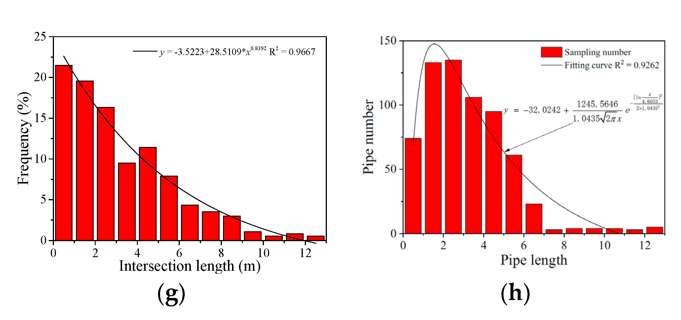
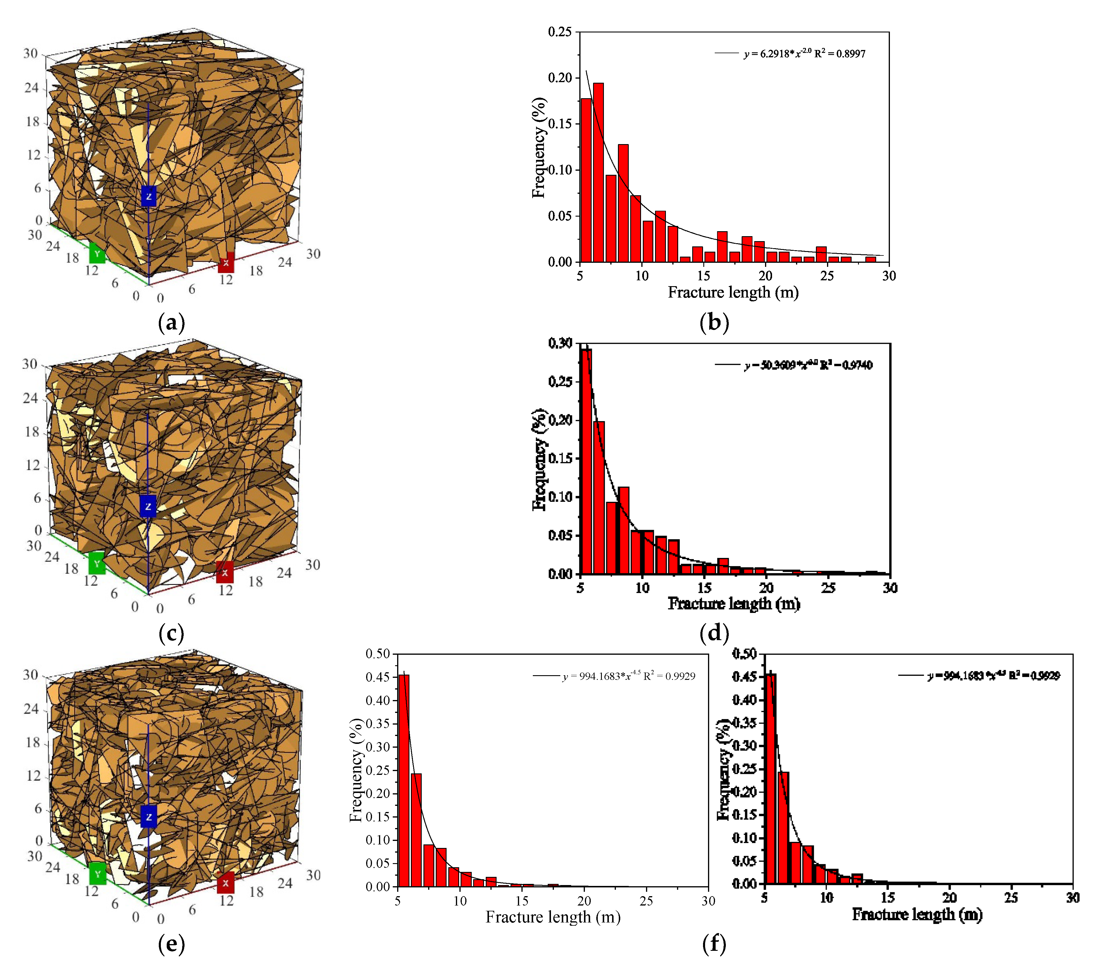
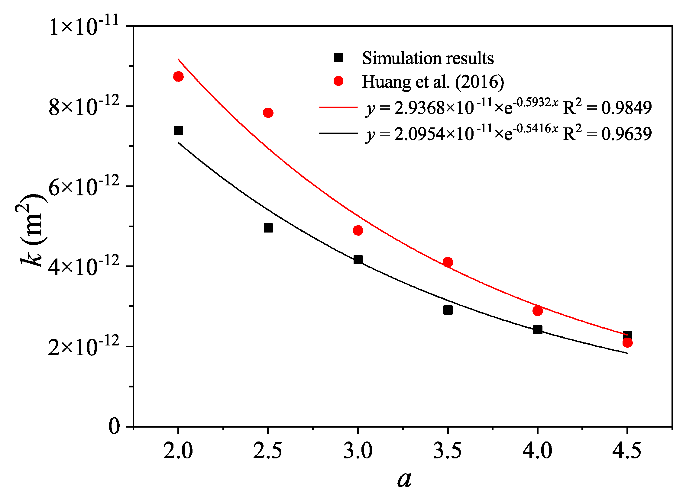
4.1. Effect of Fracture Length Distribution

The statistical geometrical parameters of fractures have a significant influence on the topology and connectivity of the fracture network and consequently affect the hydraulic properties. The exponential distribution function has been employed for describing the frequency distribution of geometrical properties of fractures [26,41]. To investigate the effect of fracture length on k, the mean value of fracture lengths (u) that follow the exponential distribution is changed from 3 m to 13 m, as shown in Figure 7, while other geometrical parameters are kept the same as those shown in Section 2.2. The k of the 3D DFN models was computed using EPN models. Figure 7 shows typical 3D DFN models and corresponding EPN models, in which u increases from 3 m to 13 m. With the increment of u, the mass density of fractures and number of pipes increase obviously. The intersection lines of DFN models can be approximately fitted by exponential functions, as shown in Figure 8a, and the R² is larger than 0.91, as tabulated in

Table 2. Parameters of fitting curves shown in Figure 8a.

u (m)	c	d	h	R2
3	−1.2557	−47.1492	0.7142	0.9860
4	−1.2333	−39.4450	0.7509	0.9797
5	−3.0247	−33.2154	0.8193	0.9533
6	−2.9572	−32.6267	0.8611	0.9764
7	−0.7913	−34.2912	0.7688	0.9701
8	−3.7502	−31.3042	0.8412	0.9641
9	−4.0304	−30.3075	0.8516	0.9767
10	−13.6517	−34.8342	0.9271	0.9197
11	−12.5329	−33.6306	0.9242	0.9567
12	−3.4822	−28.4039	0.8546	0.9540
13	−3.8291	−28.1998	0.8611	0.9472

. The intersection is a key factor of fracture connectivity because it is the connectivity of two fractures. The total intersection number and average intersection length (L_i) were calculated and plotted in Figure 8b,c, respectively. The results show that both intersection number and L_i increase as u increases, following exponential functions with R² > 0.92. To characterize the effect of fracture length on k, the dip directions and dip angles in the DFN models shown in Figure 7 were generated with the same random number seed. The stereonet map for characterizing dip directions and dip angles is shown in Figure 8d and clearly exhibits the directional characteristics of fractures located in the DFN models. The radial axis (dip direction) and lateral axis (dip angle) are equally divided into 24 and 6 intervals, respectively.

The fracture density is a significant index of fracture connectivity. Different methods have been used to determine the density of fractures according to available field data in previous studies. One of the classical parameters is P₃₂, which is defined as the total area of fracture surface per unit volume [47]. As shown in Figure 9a, the P₃₂ increases exponentially with the increment of u. This is because the increment of u leads to the increment of the number of relatively long fractures. As a result, the k increases with increasing P₃₂ when the fractures are assigned the same aperture. The relationship between k and P₃₂ can be fitted by a power-law function, as shown in Figure 9b, and the R² is larger than 0.99. The k of DFN models is not only related to P₃₂ but also associated with other geometrical parameters such as u. The relationship between u and k is depicted in Figure 9c. As u increases from 3 m to 13 m, the k increases by approximately 2 orders of magnitude from 7.5119 × 10⁻¹⁶ m² to 6.4244 × 10⁻¹⁴ m². The increment of P₃₂ induced by the increment of u can lead to the increment of k, yet P₃₂ is not the only factor affecting the magnitude of k.

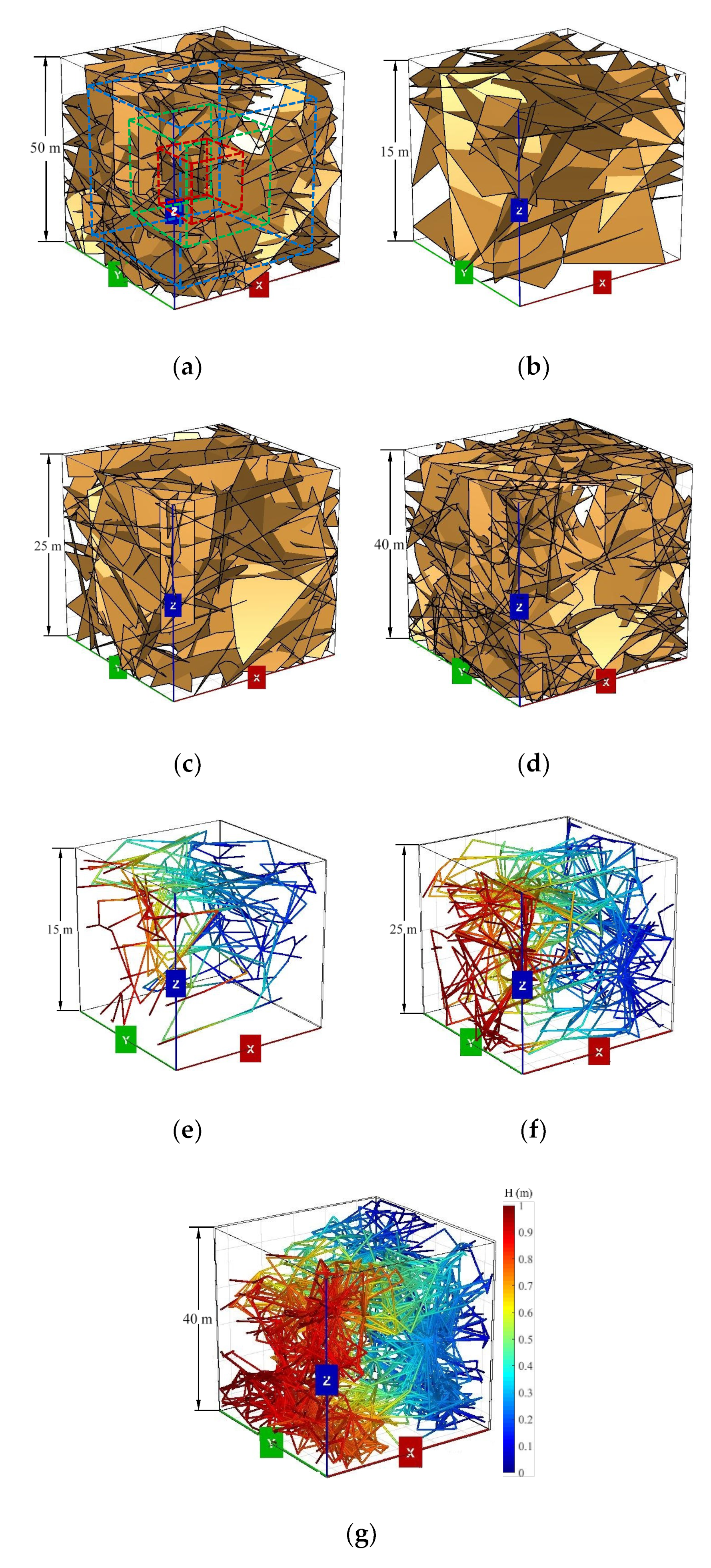
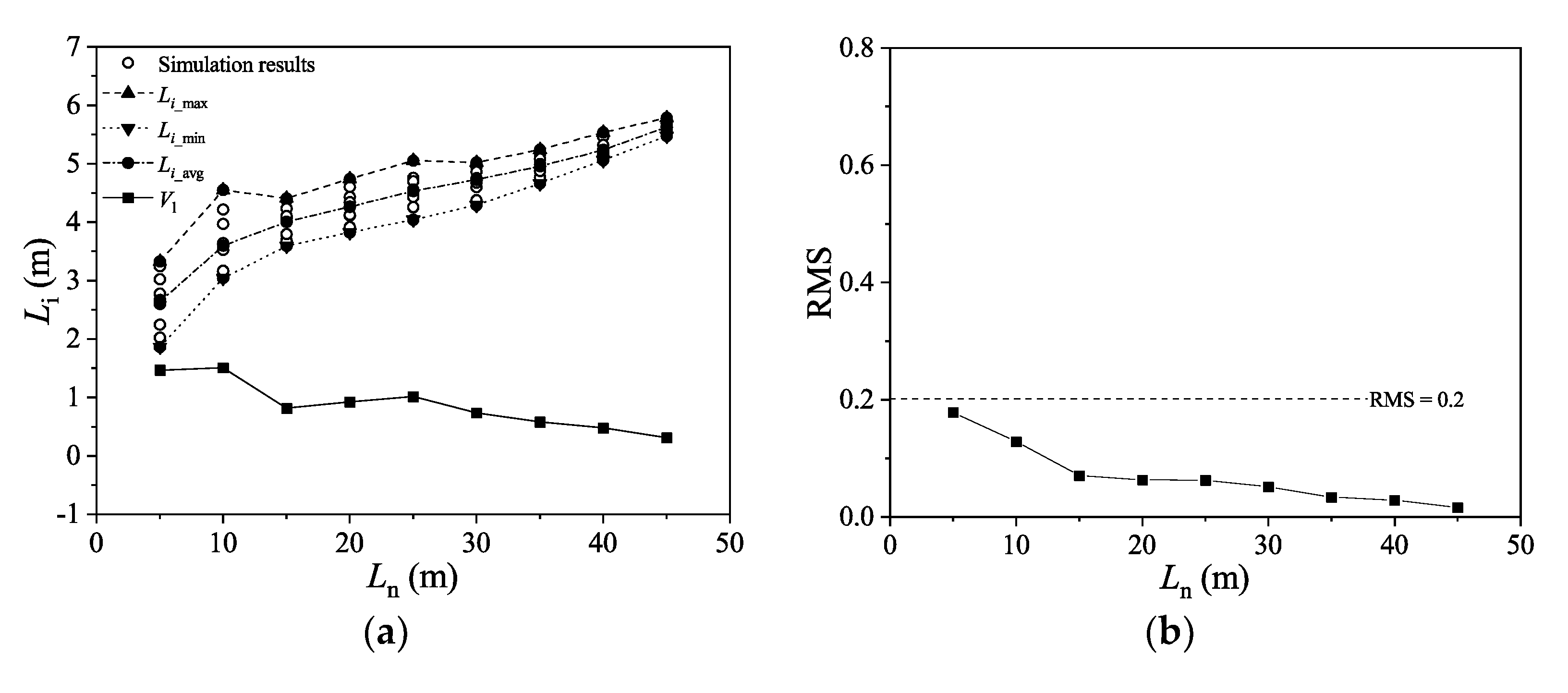
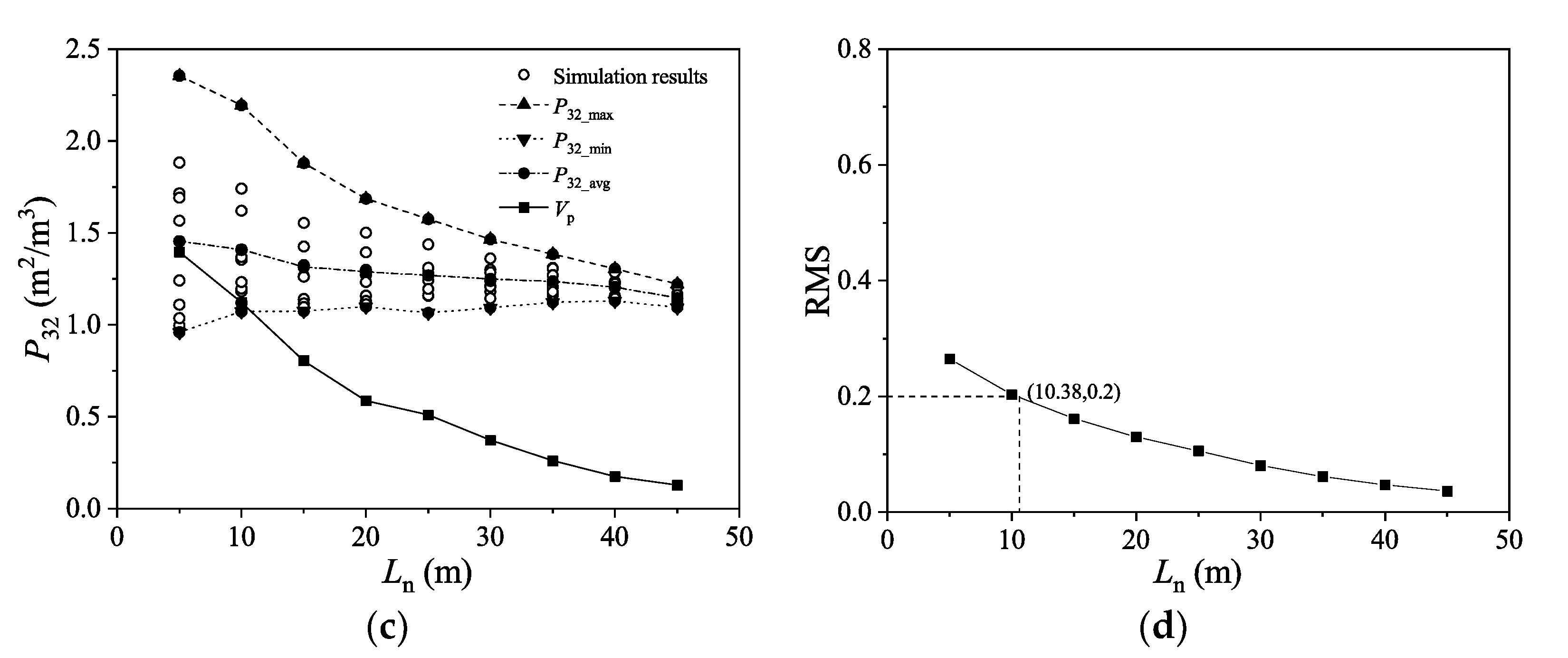
4.2. Estimation of REV Size

The REV size can be termed as a certain sample size (area in 2D and/or volume in 3D) of fractured rock masses with respect to fluid flow behavior, after which the variation in permeability changes slightly and can be negligible [48,49]. To characterize the REV of fracture networks, three original DFN models with different randomness and the same statistical geometry parameters were established, as shown in Figure 10a,c,e, in which the fracture length follows the exponential distribution. The side lengths of the 3 original DFN models are all 50 m. The fracture lengths are distributed between 5 m and 30 m with a mean value of 9 m. The aperture of fractures is set to be a constant of 1 mm. The fracture dip directions and dip angles are assumed to follow Fisher distributions in the ranges of [0, 2π) and [0, π/2), as shown in Figure 10b,d,f, respectively. The three stereonet maps clearly show the differences in the dip directions and dip angles of fractures in corresponding DFN models that were generated with different random number seeds and the same statistical geometry parameters.

The sub-models are extracted from original DFN models with side lengths (L_n) ranging from 5–45 m with an interval of 5 m. Figure 11 shows the process of extracting cube sub-models from an original DFN. The directional k is calculated by applying a constant hydraulic gradient to the opposing sides for the DFN sub-model (see Figure 12a). Figure 12b,d,f show the process of employing pressure heads in different directions, and the corresponding water head distributions are presented in Figure 12c,e,g.

The 3 hydraulic boundary conditions are taken into account: the left side is inlet with H = 1 m, and the right side is outside with a free boundary (H = 0 m); front side is inlet with H = 1 m, and the backside is outside with a free boundary (H = 0 m); top side is inlet with H = 1 m, and the bottom side is outside with a free boundary (H = 0 m). The other boundaries are assumed to be impermeable while the fluid flows through the opposite boundaries. The three hydraulic boundary conditions are presented in Figure 12b,d,f, respectively. Therefore, there are 30 directional k coefficients for each L_n, in which the k was calculated 10 times for each model corresponding to the 3 flow directions. Fluid flow in a total of 300 DFNs with different L_n and boundary conditions was simulated.

Figure 13 shows the variations in L_i and P₃₂ of cubic sub-models with different L_n and corresponding root mean square (RMS), which is defined as the square root of the average of squares of a set of values [50], was calculated and presented. As shown in Figure 13a, with increasing L_n from 5 m to 50 m, L_i changes significantly (i.e., L_n < 15 m) and then slightly (i.e., L_n ≥ 15 m). This is because in the sub-model with a small L_n, the fractures may be truncated by the boundaries, which generates smaller L_i, compared with the sub-model with a larger L_n in which the probability of the fractures being truncated is significantly decreased. Figure 13b exhibits the variations in L_i of different random number seeds; the results show that the RMS of L_i decreases with the increment of L_n. The P₃₂ is more sensitive to the randomness under a smaller L_n, as shown in Figure 13c, since the fractures are uniformly and randomly distributed in the original DFN models. The P₃₂ under a large L_n can achieve fewer differences compared to the P₃₂ under a small L_n since the volume of the former is more likely to achieve the REV size, as shown in Figure 13d. Figure 14 shows the variations in k of cube sub-models with different L_n. When L_n is small, k varies significantly due to the influence of random numbers utilized to generate fracture locations and orientations. When L_n exceeds certain values, k holds constants despite flow direction, in which the model scale can be regarded as the REV size (V_REV). RMS = 0.2 is utilized as the threshold value to determine V_REV [46]. The values of k decrease drastically up to model lengths of 28.9 m, 20.9 m, and 23.2 m and vary in a relatively small range afterward in flow direction 1, flow direction 2, and flow direction 3, respectively. The k approximately equals 5.5634 × 10⁻¹¹ m², 3.6074 × 10⁻¹¹ m^2, and 5.3759 × 10⁻¹¹ m² for the 3 flow directions when RMS = 0.2. The REV sizes are reached at the approximated V_REV sizes of 2.36 × 10⁴ m³, 9.16 × 10³ m^3, and 1.26 × 10⁴ m³ in flow direction 1, flow direction 2, and flow direction 3, respectively. The k is becoming less scattered with increasing L_n, with a clear tendency to reach a REV size. The changes in L_i and P₃₂ coincide well with those of k with the increment of L_n, as shown in Figure 13b,d, and they all change from being sharp to flat. However, the L_n equals 10.4 m for P₃₂ when RMS = 0.2 and the RMS of L_i is always less than 0.2. The dispersibility of k after the RMS of L_i and P_32, both less than 0.2, shows clearly that the significant anisotropic of the fracture network induces the differences of k in the 3 directions. Therefore, the changes of L_i or P₃₂ are unsuited to determine the REV size of the fracture network. It is necessary to focus on the modeling of fluid flow in different directions through 3D DFN models with various geometry characteristics.

5. Discussion

Our simulation results demonstrate the validity of the EPN for characterizing fluid flow through 3D DFN models. As shown in Figure 4 and Figure 6, the numerically calculated k using EPN agrees well with the analytical solutions and simulation results reported in the literature. In addition, extensive numerical simulations are performed to investigate the effect of fracture length on the properties of large-scale fracture networks. Our results show that the k increases exponentially with increasing u from 3 m to 13 m by approximately 2 orders of magnitude (Figure 9c). This trend is consistent with previous studies on solute transport and fluid flow in fracture networks under natural flow conditions [9].

At present, the degree of the effect of fracture length on the total intersection number, average intersection length, and fracture density is often ignored. Our results confirm that the P₃₂ increases following an exponent function by approximately 2.6 times as u increases (Figure 9b). And with the increment of u, the L_i and number of intersections both increase in a power-law way by approximately 1.5 and 3.4 times (Figure 8b,c, respectively. It is obvious that the influence of fracture length on the permeability of the fracture network is more significant than that on the geometric parameters, including L_i, number of intersections, and P₃₂.

The variation ranges of L_i and P₃₂ decrease gradually with the increment of the side length of DFN models, with a clear tendency to reach a REV size. A similar situation appears in the variation of k calculated by the EPN method with increasing side length. However, the dispensability of k after the RMS of L_i and P_32, both less than 0.2, implies the significant anisotropic of the fracture network. Therefore, the changes of L_i or P₃₂ are unsuited to determine the REV size of the fracture network. Moreover, the difference in REV sizes in different flow directions shows the necessity to focus on the modeling of fluid flow in different directions through 3D DFN models with various geometry characteristics.

6. Conclusions

The present study proposed an equivalent pipe network modeling approach for characterizing fluid flow through 3D fracture networks. The validity of the proposed approach is verified by comparisons with analytical results of four simple fracture network models and six complex fracture network models. Finally, extensive numerical simulations were performed to investigate the geometrical and hydraulic properties of large-scale fracture networks, and the representative elementary volume (REV) size was determined by calculating the variations in permeability (k) for fluid flow through different directions.

The results show that the permeability calculated by equivalent pipe network (EPN) models agrees well with the analytical solutions of simplified discrete fracture network (DFN) models and the simulation results of complex DFN models reported in the literature, verifying the validity of the proposed equivalent pipe network modeling approach. With the increasing average length of fracture length (u) from 3 m to 13 m, in which u denotes the mean value of fracture lengths that follow the exponential distribution, the k increases exponentially by approximately 2 orders of magnitude. The P₃₂, which is positively correlated to k, increases following an exponent function by approximately 2.6 times as u increases. The L_i and number of intersections both increase in a power-law way by approximately 1.5 and 3.4 times with the increment of u, respectively. It is obvious that the influence of fracture length on the permeability of the fracture network is more significant than that on the geometric parameters, including L_i, number of intersections, and P_32. The variation range of k decreases gradually with the increment of the side length of DFN models. The REV size of the 3D DFN model with u = 9 m determined by the values of k in different directions is calculated to be approximately 2.36 × 10⁴ m³, 9.16 × 10³ m^3, and 1.26 × 104 m³ when the root mean square equals 0.2. When the root mean squares of L_i and P₃₂ are less than 0.2, the anisotropy of fracture networks has a significant influence on the k in 3 directions, resulting in a larger representative elementary volume of the 3D DFN model than that when the root mean square of P₃₂ equals 0.2.

The equivalent pipe network is the best to simulate the fluid flow through fresh granite or shale with a complex fracture network, in which the rock matrix has very low permeability, and large-scale fluid flow is only possible through fractures. This is because large numbers of fractures expectedly result in so much complexity in interconnectivity between fractures and other characteristics that the traditional mesh unit division method will lead to low computational efficiency or even be unable to calculate. A future study will focus on establishing a model which can consider the permeability of fracture and matrix.

References

1. Gangi, A.F. Variation of whole and fractured porous rock permeability with confining pressure. Int. J. Rock Mech. Min. Sci. Geomech. Abstr. 1978, 15, 249–257. [Google Scholar] [CrossRef]
2. Brown, S.R.; Scholz, C.H. Closure of random elastic surfaces in contact. J. Geophys. Res. Solid Earth 1985, 90, 5531–5545. [Google Scholar] [CrossRef]
3. Brown, S.R. Fluid flow through rock joints: The effect of surface roughness. J. Geophys. Res. Solid Earth 1987, 92, 1337–1347. [Google Scholar] [CrossRef]
4. Berkowitz, B. Characterizing flow and transport in fractured geological media: A review. Adv. Water Resour. 2002, 25, 861–884. [Google Scholar] [CrossRef]
5. Min, K.; Jing, L.; Stephansson, O. Determining the equivalent permeability tensor for fractured rock masses using a stochastic REV approach: Method and application to the field data from Sellafield, UK. Hydrogeol. J. 2004, 12, 497–510. [Google Scholar] [CrossRef]
6. Baghbanan, A.; Jing, L. Hydraulic properties of fractured rock masses with correlated fracture length and aperture. Int. J. Rock Mech. Min. Sci. 2007, 44, 704–719. [Google Scholar] [CrossRef]
7. Baghbanan, A.; Jing, L. Stress effects on permeability in a fractured rock mass with correlated fracture length and aperture. Int. J. Rock Mech. Min. Sci. 2008, 45, 1320–1334. [Google Scholar] [CrossRef]
8. Gale, J.F.W.; Laubach, S.E.; Olson, J.E.; Eichhuble, P.; Fall, A. Natural fractures in shale: A review and new observations. AAPG Bull. 2014, 98, 2165–2216. [Google Scholar] [CrossRef]
9. Huang, N.; Jiang, Y.; Li, B.; Liu, R. A numerical method for simulating fluid flow through 3-D fracture networks. J. Nat. Gas Sci. Eng. 2016, 33, 1271–1281. [Google Scholar] [CrossRef] [Green Version]
10. Wang, G.; Qin, X.; Han, D.; Liu, Z. Study on seepage and deformation characteristics of coal microstructure by 3D reconstruction of CT images at high temperatures. Int. J. Min. Sci. Technol. 2021, 31, 175–185. [Google Scholar] [CrossRef]
11. Thanh, H.V.; Sugai, Y.; Nguele, R.; Sasaki, K. Integrated workflow in 3D geological model construction for evaluation of CO2 storage capacity of a fractured basement reservoir in Cuu Long Basin, Vietnam. Int. J. Greenh. Gas Control 2019, 90, 102826. [Google Scholar] [CrossRef]
12. Neuman, S.P. Trends, prospects and challenges in quantifying flow and transport through fractured rocks. Hydrogeol. J. 2005, 13, 124–147. [Google Scholar] [CrossRef]
13. Rothert, E.; Shapiro, S. Statistics of fracture strength and fluid-induced microseismicity. J. Geophys. Res. 2007, 112, 1–16. [Google Scholar] [CrossRef]
14. De Dreuzy, J.R.; Méheust, Y.; Pichot, G. Influence of fracture scale heterogeneity on the flow properties of three-dimensional discrete fracture networks (DFN). J. Geophys. Res. Solid Earth 2012, 117, 1–21. [Google Scholar] [CrossRef] [Green Version]
15. Fitch, P.J.R.; Lovell, M.A.; Davies, S.J.; Pritchard, T.; Harvey, P.K. An integrated and quantitative approach to petrophysical heterogeneity. Mar. Pet. Geol. 2015, 63, 82–96. [Google Scholar] [CrossRef] [Green Version]
16. Wang, T.; Zhan, S.; Huang, T. Determining transmissivity of fracture sets with statistical significance using single-borehole hydraulic tests: Methodology and implementation at Heshe well site in central Taiwan. Eng. Geol. 2015, 198, 1–15. [Google Scholar] [CrossRef]
17. Zhang, F.; Damjanac, B.; Maxwell, S. Investigating hydraulic fracturing complexity in naturally fractured rock masses using fully coupled multiscale numerical modeling. Rock Mech. Rock Eng. 2019, 52, 5137–5160. [Google Scholar] [CrossRef]
18. Liu, R.; He, M.; Huang, N.; Jiang, Y.; Yu, L. Three-dimensional double-rough-walled modeling of fluid flow through self-affine shear fractures. J. Rock Mech. Geotech. Eng. 2020, 12, 41–49. [Google Scholar] [CrossRef]
19. Hu, M.; Rutqvist, J. Multi-scale coupled processes modeling of fractures as porous, interfacial and granular systems from rock images with the numerical manifold method. Rock Mech. Rock Eng. 2021, 1–19. [Google Scholar] [CrossRef]
20. Dershowitz, W.S.; Fidelibus, C. Derivation of equivalent pipe network analogues for three-dimensional discrete fracture networks by the boundary element method. Water Resour. Res. 1999, 35, 2685–2691. [Google Scholar] [CrossRef]
21. Maillot, J.; Davy, P.; Le Goc, R.; Darcel, C.; De Dreuzy, J.R. Connectivity, permeability, and channeling in randomly distributed and kinematically defined discrete fracture network models. Water Resour. Res. 2016, 52, 8526–8545. [Google Scholar] [CrossRef] [Green Version]
22. Viswanathan, H.S.; Hyman, J.D.; Karra, S.; O’Malley, D.; Srinivasan, S.; Hagberg, A.; Srinivasan, G. Advancing graph-based algorithms for predicting flow and transport in fractured rock. Water Resour. Res. 2018, 54, 6085–6099. [Google Scholar] [CrossRef]
23. Ashraf, U.; Zhang, H.; Anees, A.; Mangi, H.N.; Zhang, X. Application of unconventional seismic attributes and unsupervised machine learning for the identification of fault and fracture network. Appl. Sci. 2020, 10, 3864. [Google Scholar] [CrossRef]
24. Jiang, R.; Zhao, L.; Xu, A.; Ashraf, U.; Yin, J.; Song, H.; Su, N.; Du, B.; Anees, A. Sweet spots prediction through fracture genesis using multi-scale geological and geophysical data in the karst reservoirs of Cambrian Longwangmiao Carbonate Formation, Moxi-Gaoshiti area in Sichuan Basin, South China. J. Pet. Explor. Prod. Technol. 2021, 12, 1313–1328. [Google Scholar] [CrossRef]
25. Doolaeghe, D.; Davy, P.; Hyman, J.D.; Darcel, C. Graph-based flow modeling approach adapted to multiscale discrete-fracture-network models. Phys. Rev. E 2020, 102, 53312. [Google Scholar] [CrossRef]
26. De Dreuzy, J.R.; Davy, P.; Bour, O. Percolation parameter and percolation-threshold estimates for three-dimensional random ellipses with widely scattered distributions of eccentricity and size. Phys. Rev. E 2000, 62, 5948–5952. [Google Scholar] [CrossRef] [Green Version]
27. Cruden, D.M. Describing the size of discontinuities. Int. J. Rock Mech. Min. Sci. 1977, 14, 133–137. [Google Scholar] [CrossRef]
28. Hudson, J.A.; Priest, S.D. Discontinuities and rock mass geometry. Int. J. Rock Mech. Min. Sci. Geomech. Abstr. 1979, 16, 339–362. [Google Scholar] [CrossRef]
29. Priest, S.D.; Hudson, J.A. Estimation of discontinuity spacing and trace length using scanline surveys. Int. J. Rock Mech. Min. Sci. Geomech. Abstr. 1981, 18, 183–197. [Google Scholar] [CrossRef]
30. Cowie, P.A.; Scholz, C.H.; Edwards, M.; Malinverno, A. Fault strain and seismic coupling on mid-ocean ridges. J. Geophys. Res. Solid Earth 1993, 98, 17911–17920. [Google Scholar] [CrossRef]
31. Carbotte, S.M.; Macdonald, K.C. Comparison of seafloor tectonic fabric at intermediate, fast, and super fast spreading ridges: Influence of spreading rate, plate motions, and ridge segmentation on fault patterns. J. Geophys. Res. Solid Earth 1994, 99, 13609–13631. [Google Scholar] [CrossRef]
32. Bonnet, E.; Bour, O.; Odling, N.E.; Davy, P.; Main, I.; Cowie, P.; Berkowitz, B. Scaling of fracture systems in geological media. Rev. Geophys. 2001, 39, 347–383. [Google Scholar] [CrossRef] [Green Version]
33. Zhang, L.; Einstein, H.H.; Dershowitz, W.S. Stereological relationship between trace length and size distribution of elliptical discontinuities. Géotechnique 2002, 52, 419–433. [Google Scholar] [CrossRef]
34. Agosta, F.; Alessandroni, M.; Antonellini, M.; Tondi, E.; Giorgioni, M. From fractures to flow: A field-based quantitative analysis of an outcropping carbonate reservoir. Tectonophysics 2010, 490, 197–213. [Google Scholar] [CrossRef]
35. Bustin, A.M.M.; Bustin, R.M. Importance of rock properties on the producibility of gas shales. Int. J. Coal Geol. 2012, 103, 132–147. [Google Scholar] [CrossRef]
36. Cowie, P.A.; Sornette, D.; Vanneste, C. Multifractal scaling properties of a growing fault population. Geophys. J. R. Astron. Soc. 2010, 122, 457–469. [Google Scholar] [CrossRef] [Green Version]
37. Long, J.C.S.; Remer, J.S.; Wilson, C.R.; Witherspoon, P.A. Porous media equivalents for networks of discontinuous fractures. Water Resour. Res. 1982, 18, 645–658. [Google Scholar] [CrossRef] [Green Version]
38. Zhou, F.; Tang, Z. Discrete fracture network modelling in a naturally fractured carbonate reservoir in the Jingbei oilfield, China. Energies 2017, 10, 183. [Google Scholar]
39. Priest, S.D. Discontinuity Analysis for Rock Engineering; Chapman & Hall: London, UK, 1993. [Google Scholar] [CrossRef]
40. Hyman, J.D.; Karra, S.; Makedonska, N.; Gable, C.W.; Painter, S.L.; Viswanathan, H.S. dfnWorks: A discrete fracture network framework for modeling subsurface flow and transport. Comput. Geosci. 2015, 84, 10–19. [Google Scholar] [CrossRef] [Green Version]
41. Cacas, M.C.; Ledoux, E.; De Marsily, G.; Tillie, B.; Durand, E.; Feuga, B.; Peaudecerf, P. Modeling fracture flow with a stochastic discrete fracture network: Calibration and validation: 1. The flow model. Water Resour. Res. 1990, 26, 479–489. [Google Scholar] [CrossRef]
42. Nordqvist, A.W.; Tsang, Y.W.; Tsang, C.F.; Dverstorp, B.; Andersson, J. A variable aperture fracture network model for flow and transport in fractured rocks. Water Resour. Res. 1992, 28, 1703–1713. [Google Scholar] [CrossRef]
43. Xu, C.; Fidelibus, C.; Dowd, P. Realistic Pipe Models for Flow Modelling in Discrete Fracture Networks. In Proceedings of the First International Discrete Fracture Network Engineering Conference, Vancouver, BC, Canada, 19–22 October 2014. [Google Scholar]
44. Alghalandis, Y.F. ADFNE: Open source software for discrete fracture network engineering, two and three dimensional applications. Comput. Geosci. 2017, 102, 1–11. [Google Scholar] [CrossRef]
45. Xu, W.; Zhang, Y.; Li, X.; Wang, X.; Zhang, P. Study on three-dimensional fracture network connectivity path of rock mass and seepage characteristics based on equivalent pipe network. Environ. Earth Sci. 2019, 78, 516. [Google Scholar] [CrossRef]
46. Dverstorp, B.; Andersson, J.; Nordqvist, W. Discrete fracture network interpretation of field tracer migration in sparsely fractured rock. Water Resour. Res. 1992, 28, 2327–2343. [Google Scholar] [CrossRef]
47. Davy, P.; Darcel, C.; Bour, O.; Munier, R.; De Dreuzy, J.R. A note on the angular correction applied to fracture intensity profiles along drill core. J. Geophys. Res. Solid Earth 2006, 111, B11408. [Google Scholar] [CrossRef] [Green Version]
48. Panda, B.B.; Kulatilake, P. Effect of joint geometry and transmissivity on jointed rock hydraulics. J. Eng. Mech. 1999, 125, 41–50. [Google Scholar] [CrossRef]
49. Kulatilake, P.; Panda, B.B. Effect of block size and joint geometry on jointed rock hydraulics and REV. J. Eng. Mech. 2000, 126, 850–858. [Google Scholar] [CrossRef]
50. Ohman, J.; Niemi, A. Upscaling of fracture hydraulics by means of an oriented correlated stochastic continuum model. Water Resour. Res. 2003, 39, 71. [Google Scholar] [CrossRef] [Green Version]
Figure 1. Fracture network model and corresponding geometric and hydraulic properties. (a) Three-dimension DFN model; (b) Intersections; (c) Pipe structure; (d) Backbone structure; (e) Graph structure (nodes and edges); (f) Water head distribution; (g) Frequency distribution of fracture lengths; (h) Frequency distribution of pipe lengths.
Water 14 01582 g001aWater 14 01582 g001b
Figure 2. Schematic view of equivalent pipes of rock fractures.
Water 14 01582 g002
Figure 3. DFN models, EPN models, and simplified DFN models. (a) The DFN model with one fracture; (b) The EPN model extracted from Figure 3a; (c) The simplified DFN model extracted from Figure 3a; (d) The DFN model with two fractures; (e) The EPN model extracted from Figure 3d; (f) The simplified DFN model extracted from Figure 3d; (g) The DFN model with four fractures; (h) The EPN model extracted from Figure 3g; (i) The simplified DFN model extracted from Figure 3g; (j) The DFN model with six fractures; (k) The EPN model extracted from Figure 3j; (l) The simplified DFN model extracted from Figure 3j.
Water 14 01582 g003aWater 14 01582 g003b
Figure 4. Comparisons of k calculated using the EPN models and the simplified DFN models, and the variations in ε versus number of fractures.
Water 14 01582 g004
Figure 5. Three-dimension DFN models and corresponding statistical histograms of the fracture length with different a when P32 = 0.4. (a) The DFN model when a = 2.0; (b) The distribution of fracture length when a = 2.0; (c) The DFN model when a = 3.0; (d) The distribution of fracture length when a = 3.0; (e) The DFN model when a = 4.5; (f) The distribution of fracture length when a = 4.5.
Water 14 01582 g005
Figure 6. Comparisons of k between the simulation results calculated using the EPN models and results reported by Huang et al. [9].
Water 14 01582 g006
Figure 7. Representative three-dimension DFN models and corresponding EPN models for different u. (a) The DFN model when u = 3 m; (b) The EPN model when u = 3 m; (c) The DFN model when u = 5 m; (d) The EPN model when u = 5 m; (e) The DFN model when u = 7 m; (f) The EPN model when u = 7 m; (g) The DFN model when u = 9 m; (h) The EPN model when u = 9 m; (i) The DFN model when u = 11 m; (j) The EPN model when u = 11 m; (k) The DFN model when u = 13 m; (l) The EPN model when u = 13 m.
Water 14 01582 g007
Figure 8. Geometrical properties of intersections for the DFN models shown in Figure 6. (a) Frequency distributions of intersection lengths; (b) Relationship between number of intersections and u; (c) Relationship between Li and u; (d) Stereonet map of dip directions and dip angles.
Water 14 01582 g008aWater 14 01582 g008b
Figure 9. Relationships among P32, u, and k. (a) Relationship between P32 and u; (b) Variation in k with P32; (c) Relationship between k and u.
Water 14 01582 g009
Figure 10. DFN models generated using three sets of random numbers and corresponding stereonet maps of dip directions and dip angles. (a) DFN model for set 1; (b) Dip directions and dip angles for set 1; (c) DFN model for set 2; (d) Dip directions and dip angles for set 2; (e) DFN model for set 3; (f) Dip directions and dip angles for set 3.
Water 14 01582 g010
Figure 11. Extracted sub-models from the original cube DFN model. (a) Original cube DFN model (Ln = 50 m); (b) Sub-model (Ln = 15 m); (c) Sub-model (Ln = 25 m); (d) Sub-model (Ln = 40 m); (e) EPN model (Ln = 15 m); (f) EPN model (Ln = 25 m); (g) EPN model (Ln = 40 m).
Water 14 01582 g011
Figure 12. Hydraulic boundary conditions of sub-models and corresponding distributions of water heads. (a) A simple DFN sub-model; (b) Flow direction 1; (c) Water head distribution for flow direction 1; (d) Flow direction 2; (e) Water head distribution for flow direction 2; (f) Flow direction 3; (g) Water head distribution for flow direction 3.
Water 14 01582 g012
Figure 13. Variations in P32 and Li with increasing Ln. (a) Relationship between Li and Ln; (b) Relationship between RMS of Li with Ln; (c) Relationship between P32 and Ln; (d) Relationship between RMS of P32 with Ln.
Water 14 01582 g013aWater 14 01582 g013b
Figure 14. Variations in k and RMS with increasing Ln in three flow directions. (a) Variations in k in flow direction 1; (b) Variations in RMS in flow direction 1; (c) Variations in k in flow direction 2; (d) Variations in RMS in flow direction 2; (e) Variations in k in flow direction 3; (f) Variations in RMS in flow direction 3.
Water 14 01582 g014