Abstract
Anaerobic digestion (AD) is an efficient wastewater bioprocess, suitable for treating agroindustrial residues with high organic loads and characterized by both a low environmental impact and energy generation. This process is conformed by several chemical and biological reactions in an oxygen free atmosphere, that degrades high molecular weight organic compounds into carbon dioxide and methane mainly but also into traces of hydrogen and ammonia. This process is potentially unstable to volatile fatty acids (VFA), and the alkalinity. variations and is satisfactorily described by the non-linear AM2 model. In this contribution, the AM2 model is modified to include a more general expression for the pH, a cheap and continuous measurement, and also to add more detail in the interactions of the VFA, bicarbonates, and the alkalinity, key factors in the process stability. The stability of the AM2 modified model is explored through a rigorous bifurcation analysis that identifies unstable operation zones and viability of operation trajectories as a function of the dilution rate. Finally, an experimental validation is carried out to show the feasibility and accuracy of the proposed modifications.
1. Introduction
Anaerobic digestion (AD) is an appealing bioprocess for agroindustrial wastewater treatment that shows many advantages when compared to other treatments [1,2,3,4,5]. For instance, AD may have profit returns from energy production and a direct way of recycling nutrients [2,6]. However, unexpected changes in temperature, hydraulic or organic overloads and the presence of inhibitory substances may negatively affect the digester stability [7,8,9]. Under these circumstances, the digester becomes unstable due to the accumulation of volatile fatty acids (VFA) drastically lowering the digester pH (acidification) [10]. If the perturbation that produces the digester instability is not mended in an early stage, the global failure of the digestion process is expected [11,12]. This is one of the reasons why most of the researches are focused on finding new ways to improve the AD performance by implement monitoring techniques and advanced control schemes that guarantee the stability of the digester [13,14,15,16,17,18,19,20,21]. On the other hand, many other researches [1,22,23,24] are focused on the regulation of a parameter known as alkalinity to reach the stability of the digestion process, in particular, Ripley et al. [10] proposed a methodology to measure the intermediate alkalinity (IA), which evaluates alkalinity between pH 5.7 and 4.3 and in conjunction with the partial alkalinity (PA) and the total alkalinity (TA), quantify the buffer capacity in the digestor of the the VFA, bicarbonates and the sum of both, respectively, allowing to prevent the acidification and washout of the biomass of the AD process. For instance, Palacios-Ruiz et al. [22] proposed the simultaneous control of VFA and the total alkalinity in anaerobic digesters. The control scheme is conformed by an output feedback control and an extended Luenberger observer that is used to estimate the uncertainties corresponding to the controlled states, while in the literature a common variable associated to alkalinities is the IA:PA ratio.
There are several models developed in the literature to describe the AD process [1,24,25,26,27,28,29,30]. Some models [31,32] have as the main objective to display a high precision representation of the biological processes that occur during the degradation of organic matter through AD. Nevertheless, these models are characterized by a large number of equations and parameters that makes them unsuitable for practical applications on real AD processes such as estimation or control tasks. The Anaerobic Digestion Model 2 (AM2) proposed by Bernard et al. [33] is conformed by a reduced number of equations, provide an adequate precision of the AD processes by considering two biological reactions and elemental physicochemical balances, while maintaining a mathematical simplicity. Regardless of the mentioned advantages that the AM2 model presents, it does not explicitly consider the alkalinities, i.e., the partial (PA), the intermediate (IA) and the total alkalinity (TA), and their ratios. In several studies [10,16,34] it has been shown that the IA:PA and IA:AT ratios are of paramount importance for process monitoring, surveillance, and control purposes. In this regard, several robust control schemes have been proposed to regulate state variables along with the alkalinities by introducing mild modifications to the model, such that the effect of strong ions can be considered more explicitly [1,35].
On the other hand, stability analysis of mathematical models provides important information on the qualitative behavior of the system that is being modeled. For instance, the stability analysis might show not only the equilibrium regions for the system but also the detection of stable regions of the system. In other words, the stability analysis provides limit values for the main system variables that assure its stable operation. Several stability analysis have been developed [36,37,38] for a number of anaerobic digestion models whose results have been considered in the development of monitoring and robust control schemes. Thus, the main focus of this contribution is to include several modifications to the AM2 model in order to directly evaluate the IA:PA ratio and to report a bifurcation and a stability analysis of the modified model, which allows to define the stable operation zones of the process. The proposed modifications emerge from the chemical balance of the ionic species involved in the AD process and by including the pH as an additional algebraic variable, then, the relations that allow the direct evaluation of the IA:PA and IA:TA ratios are derived. This paper is organized as follows: in Section 2, the proposed modifications to the AM2 model are shown and developed for the inclusion of the alkalinity factor as a variable, in Section 3, the stability analysis of the modified model is discussed with a special focus on the results obtained on the behavior of the IA:PA and IA:TA ratios for the stable and unstable zones. Finally, in Section 4, conclusions and future work are discussed.
2. Modifications to the AM2 System
The AM2 model [33] has some of the desirable characteristics for control design, since it is a relatively simple model but with a satisfactory prediction of the AD process dynamic behavior. This model describes the acidogenesis and methanogenesis stages, contains six state variables and has the following structure:
where is the acidogenic biomass, is the methanogenic biomass, is the soluble chemical oxygen demand (COD), is the VFA concentration, is the sum of strong ions, and is the total inorganic carbon (TIC). is the dilution rate, defined as , where is the reactor volume and is the volumetric flow, is the suspended biomass fraction in the liquid phase (), , for , are yield coefficients and is the molar flow of gaseous , defined as
with as a liquid-gas mass transfer coefficient, is the disolved and not dissociated concentration, that Bernard et al. [33] assumed to be mainly the specie, as the Henry constant, and is the partial pressure of the gaseous , defined by
where , , is the total pressure in the digester, and is the methane molar flow, given by
The expression represents a Monod-type specific growth rate for acidogenic microorganisms while represents a Haldane type specific growth rate for methanogenic microorganisms, where it is assumed that the VFA at high concentrations induces microbial growth inhibition. The Monod and Haldane microorganisms growth kinetics are given respectively by
with as the maximum growth rate for acidogenic bacteria, as the half saturation constant, as the maximum growth rate for methanogenic archaea, as the half saturation constant, and as the inhibition constant.
The acidogenic balance, with the reaction is represented by
and the methanogenic balance, with the reaction is given by
where is the yield coefficient for COD degradation, is the yield coefficient for VFA production, is the yield coefficient for VFA consumption, and are the yield coefficient for production and is the yield coefficient for production.
Physicochemical Relationships
The AM2 model has been validated for several substrates and operating conditions [22,39] however, modifications can be made in its structure in order to include the process alkalinity by considering the physicochemical equilibrium of the dissociated and undissociated species and by including the effect of pH.
Considering the balance of species developed by Bernard et al. [33], the total VFA consider both dissociated and un-dissociated species, i.e.:
where and are the ionized and un-ionized acid species respectively, while the TIC can be represented as:
, , and are the carbonic acid, bicarbonate, carbonate, and the aqueous carbon dioxide concentrations, respectively. Due to the normal stable operation conditions of AD processes, in the pH range of 6–8 in [33] it was considered that the bicarbonates are partially dissociated, while the VFA are completely dissociated, i.e., and , however if the pH is different from the proposed range, i.e., pH < 6 or pH > 8, the approximation has less accuracy, therefore to measure the alkalinity using the typical methodology [10] and to include all the pH ranges operating conditions of an anaerobic digester, the full balances (12) and (13) must be considered.
To compute ion concentrations, the following equilibrium relationships are considered:
where the anions are , , and , while the common cation is .
The respective equilibrium constants under ideal conditions for each dissociation in aqueous medium are
where is the hydrogen ion concentration, and is the hydroxil concentration, while is the concentration of water that can be considered constant, therefore, it is possible to replace with constant and such that and
Thus, the hydroxil concentration can be determined through measurements. Furthermore, by requiring electroneutrality ion balance in the solution, the following equation is obtained:
Considering the derivation above, it is possible to evaluate all the chemical species concentrations as functions of both pH and the AM2 state variables as follows:
According to Bernard et al. [33], in Equation (8) the concentration is computed as , that is based on the simplified expressions for and proposed by Bernard et al. [33] for pH around 7, however for a broader region of pH, these approximations are no longer useful, thus we propose to compute with Equation (23). In addition, by using Equation (20) and the ions concentrations, it is possible to establish a direct relationship between Z and knowing and in the following form
where , , and are functions of the hydrogen ion concentration:
and similarly, a relationship to determine the amount of acid required to perform the titration at a desired pH can be defined as
where is the concentration of the strong acid titration solution required for a established pH. The (with ) is the pH established to evaluated the partial () and total () alkalinity [10].
Thus, the following relationships depicting the different alkalinities in the digestor are obtained:
where is defined as the partial alkalinity, is the total alkalinity, and is intermediate alkalinity and Z is described in Equation (27). Here
while , since this value is linked to the alkalinity due to the bicarbonates, and , since at this value the buffer capacity of both the bicarbonates and the VFA is measured [10].
The proposed modification of the AM2 model allows us to compute the alkalinities using Equations (31)–(33), however they require the pH, which can be obtained by solving the nonlinear Equation (27). To avoid this inconvenient, it is possible to replace the dynamics of the sum of strong ions (Z), i.e., the Equation (5), with the dynamics of the hydrogen ion concentration, , that has the following form:
where is the inflow hydrogen ion concentration that must satisfy the electroneutrality
Hence, it is possible to perform a process bifurcation and stability analysis that includes the partial, intermediate, total alkalinities, and IA:PA ratio as depicted in the following Section.
3. Bifurcation Analysis
The bifurcation and stability analysis are performed in equilibrium points of a nonlinear dynamical system described by ordinary or partial differential equations. The state of the system is defined by the relationships between the state variables and the parameters, which do not depend on the state variables, but these can assume different numerical values. It is important to know how variation of a parameter affects the solution of a given system, since small changes may have a drastic effect on the qualitative behavior. This is known as bifurcation [40].
The equilibrium points of the modified AM2 model that now considers the pH and the IA:PA ratio is obtained by setting the time derivatives in balances of Equations (1)–(6) equal to zero, i.e.,
where * represents the equilibrium point values. To find the equilibrium points it is also necessary to take into account Equations (7)–(9), (23) and (27). Hence, for each dilution rate, , up to six possible equilibrium points (EPi) are obtained representing:
- EP1
- The washout of both biomasses, for .
- EP2
- The washout only of the methanogenic biomass, for , with .
- EP3
- The washout of the acidogenic biomass only (with two possible equilibrium points):
- EP3a
- for , withand ,
- EP3b
- for .
- EP4
- The survival of both biomasses (with two possible equilibrium points):
- EP4a
- for withand ,
- EP4b
- for .
Notice that for a high enough COD inflow concentration, such that , it holds that , i.e., that the acidogenic biomass can survive after the washout of the methanogenic biomass, while for a small enough COD inflow concentration, such that , it holds that and even for smaller COD inflow concentrations with it holds that and EP4a completely disappears, representing that the methanogenic biomass can survive after the washout of the acidogenic biomass. Therefore, the number and position of the bifurcation points depend on the kinetic parameters and inflow concentrations.
Table 1 summarizes the process variables at each possible equilibrium. The acidogenic and methanogenic biomasses ( and ) as well as the COD (), the VFA () and the sum of strong ions () have analytical solutions for the six cases, while and must be evaluated numerically by solving the set of nonlinear equations
that depend on the other variables.

Table 1.
Equilibrium points.
Finally, the stability properties for each possible equilibrium point can be evaluated using the indirect Lyapunov method by computing the eigenvalues of the Jacobian matrix, which depends on the particular value of the parameters, the dilution rate, and the inflow concentrations.
4. Discussion
4.1. Bifurcation of an Analytical Case Study
Regarding Table 1 there could be up to 5 bifurcation points for the dilution rate: , , , , and . For these particular parameters, the dilution rates and coalesce, therefore in the bifurcation diagrams they appear as the same line. These bifurcation points can produce both changes in the number of possible equilibrium points and changes in the stability properties of these equilibrium points. Regarding the number of equilibrium points, there can be simultaneously up to 6 different equilibrium points. In particular, the behavior of both the COD and the acidogenic biomass for the total washout (EP1) and acidogenic washout (EP3a and EP3b) are identical, with and , while the behavior of the COD for the methanogenic washout (EP2) is identical to the behavior without washout (EP4a and EP4b) and equal to and , respectively. On the other hand, the behavior of both the VFA and the methanogenic biomass for the total washout (EP1) and methanogenic washout (EP2) are identical, with and , in contrast with the behavior of the VFA and the methanogenic biomass for the acidogenic washout and without washout; for these cases, the VFA in EP3a and EP4a are identical () and this VFA concentration is higher than the VFA concentration for EP3b and EP4b (), which are also identical between them, while the methanogenic biomass reaches different concentrations for all these cases (EP3a, EP3b, EP4a, and EP4b, respectively) and, given that the methane production depends on the VFA and methanogenic biomass concentrations, the methane flow rate also reaches different values for each of these cases.
Finally, since the behavior of the TIC concentration and the hydrogen ion concentration (or pH) are given by the TIC and electroneutrality balances, in Equations (35) and (36), and they depend on the behavior of the VFA and the acidogenic and methanogenic biomass concentrations, then the TIC and the hydrogen ion concentrations are different for each class of equilibrium points (EP1, EP2, EP3a, EP3b, EP4a, and EP4b, respectively) and, as a consequence, the flow rate is also different for each class of equilibrium points.
With respect to the stability properties of the model, in general for a fixed value of the dilution rate with which is the more common case, equilibrium points for total washout (EP1, ●) are unstable nodes for and they are globally asymptotically stable nodes for . Equilibrium points for washout only of the methanogenic biomass (EP2, ▪) are unstable nodes for and asymptotically stable nodes for . Equilibrium points for the first roots of both the washout only for the acidogenic biomass (EP3a, ⧫) and without washout (EP4a, ▾) are saddle points (unstable) for all their interval of existence, and , respectively, while the second roots of the washout only for the acidogenic biomass (EP3b, ★) are unstable nodes for all their interval of existence , in contrast with the second roots of the equilibrium points without washout (EP4b, ▴) that are stable nodes for all their intervals of existence .
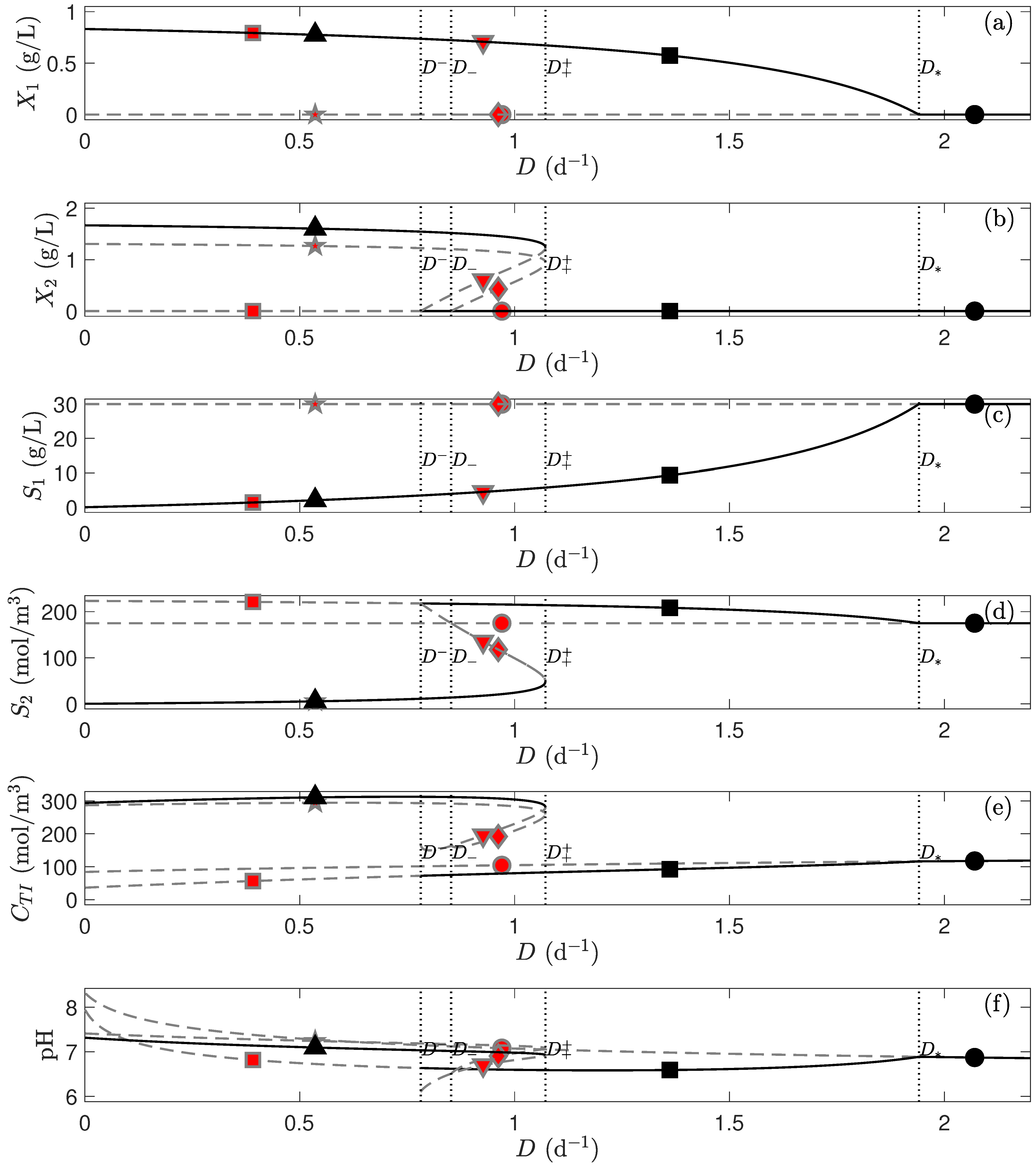
In order to illustrate a particular case of the previous discussion, Figure 1, Figure 2, Figure 3 and Figure 4 show the bifurcation analysis of the modified AM2 model using the parameters described in Table 2 [33,41], with respect to the dilution rate. In all these figures the lines represent stable equilibrium points, the dashed lines represent unstable equilibrium points and the dotted lines indicate the bifurcation points for the dilution rate; the markers represent the regions for each class of equilibrium, thus ● represents the region for EP1, ▪ for EP2, ★ for EP3a, ⧫ for EP3b, ▾ for EP4a, and ▴ for EP4b. In particular, Figure 1 shows bifurcation and stability for the state variables, thus Figure 1a,b describes the acidogenic and methanogenic biomass behavior, respectively, while Figure 1c–e shows the behavior of COD, VFA, and TIC. Finally, Figure 1f shows the predicted pH. On the other hand, Figure 2a,b shows the behavior of the methane and gas flow rates, respectively, while Figure 3a–c depicts the partial, intermediate, and the total alkalinities’ behavior, respectively. Finally, Figure 4 shows the behavior of the IA:PA ratio.
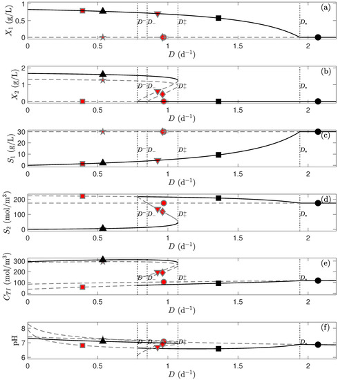
Figure 1.
Bifurcation and stability analysis of the modified AM2 model with the parameters in Table 2. (a) acidogenic biomass, (b) methanogenic biomass, (c) COD, (d) VFA, (e) CTA, and (f) pH with bifurcations at , and . The continuous lines with black markers represent stable EP, the dashed lines with red markers represent unstable EP, and the dotted lines are the bifurcation points, while the shape of markers indicates the regions for each EP: ● = EP1, ▪ = EP2, ★ = EP3a, ⧫ = EP3b, ▾ = EP4a, and ▴ = EP4b.
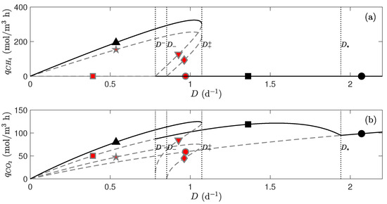
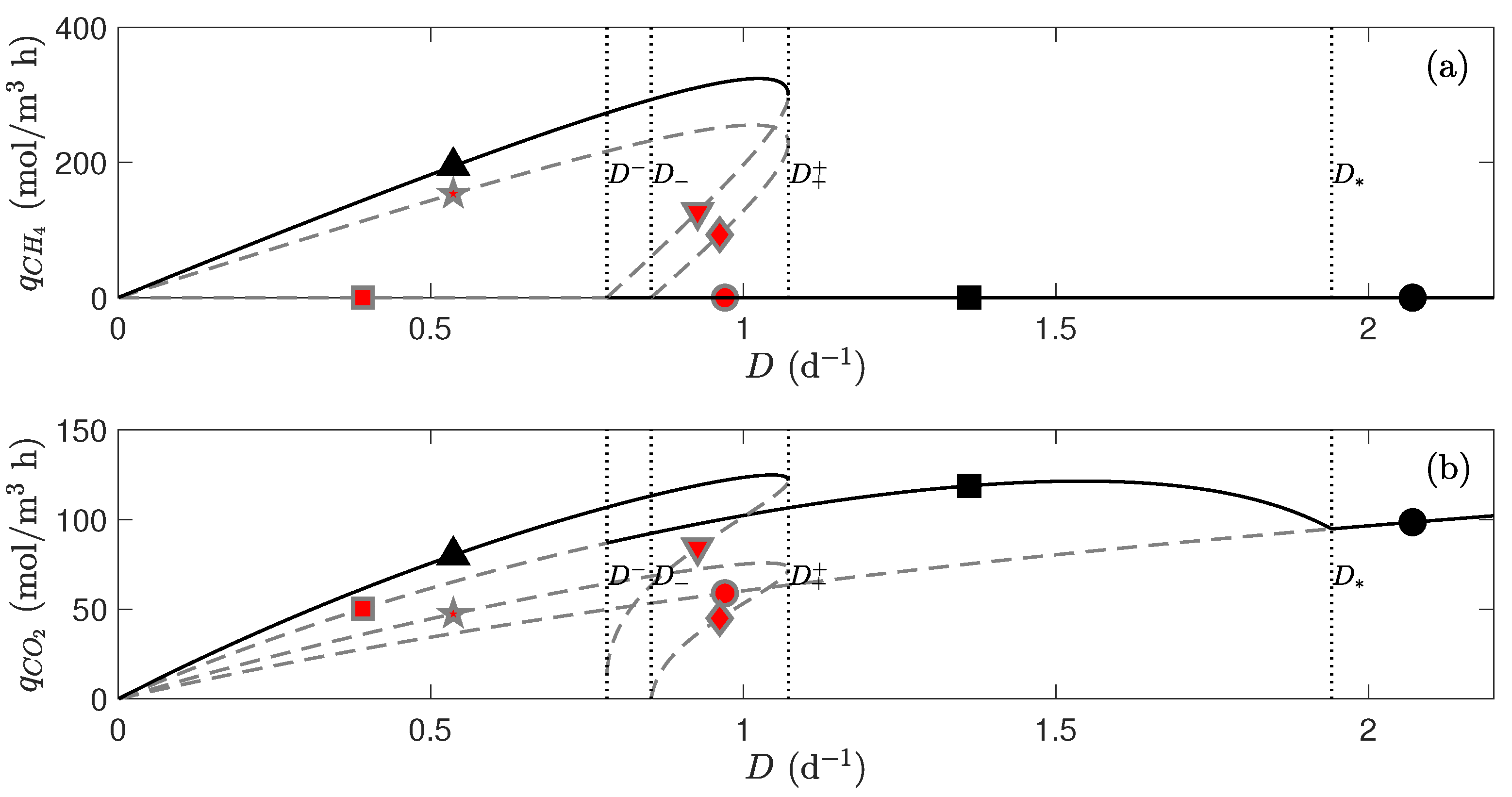
Figure 2.
Bifurcation and stability analysis for gas flows of the modified AM2 model with Table 2 parameters. (a) Methane flow and (b) flow. The continuous lines with black markers represent stable EP, the dashed lines with red markers represent unstable EP, and the dotted lines are the bifurcation points, while the shape of markers indicates the regions for each EP: ● = EP1, ▪ = EP2, ⧫ = EP3a, ★ = EP3b, ▾ = EP4a, and ▴ = EP4b.

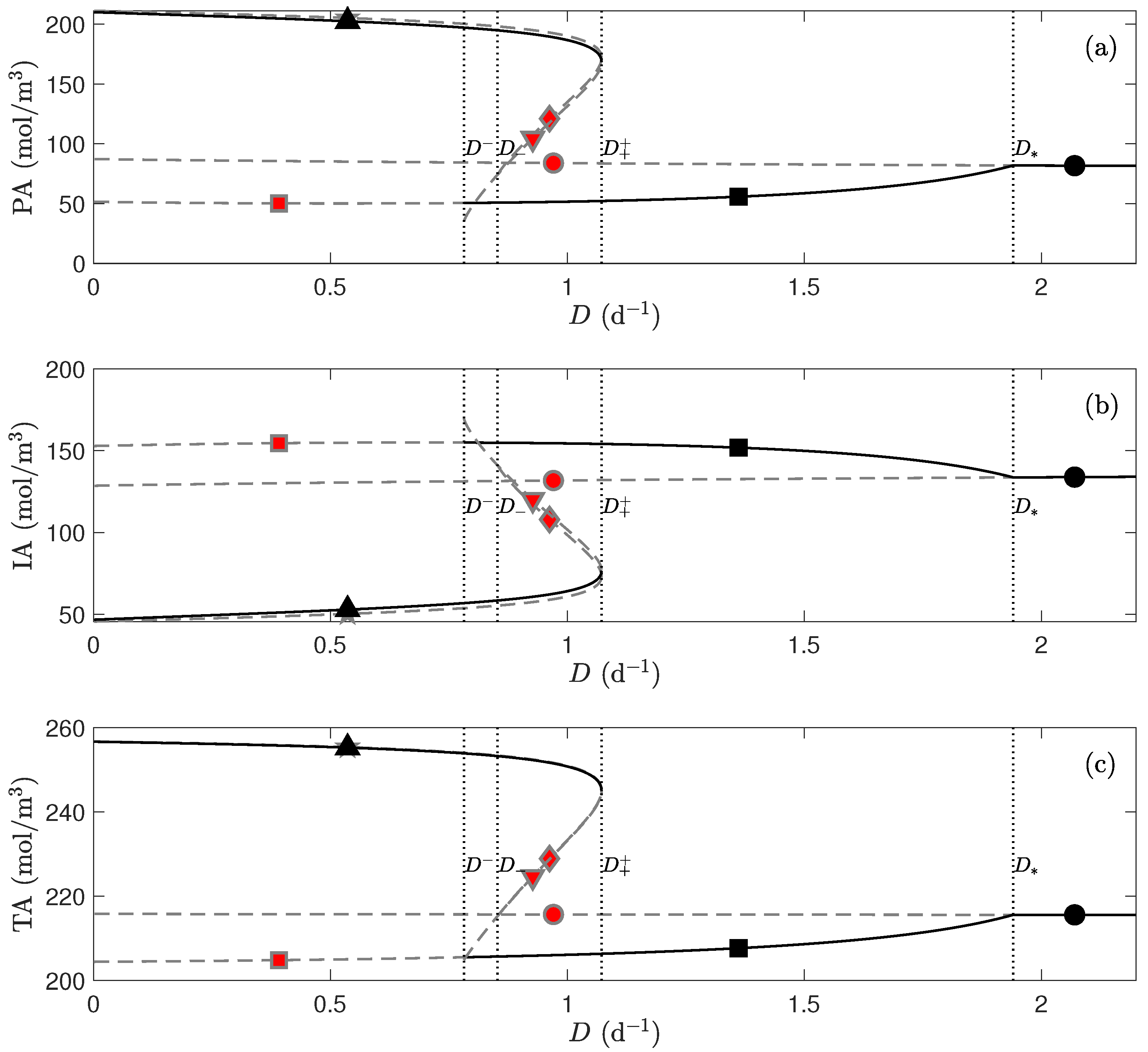
Figure 3.
Bifurcation and stability analysis for alkalinities of the modified AM2 model with the parameters in Table 2. (a) Intermediate alkalinity, (b) partial alkalinity, and (c) total alkalinity. The continuous lines with black markers represent stable EP, the dashed lines with red markers represent unstable EP, and the dotted lines are the bifurcation points, while the shape of markers indicates the regions for each EP: ● = EP1, ▪ = EP2, ⧫ = EP3a, ★ = EP3b, ▾ = EP4a, and ▴ = EP4b.
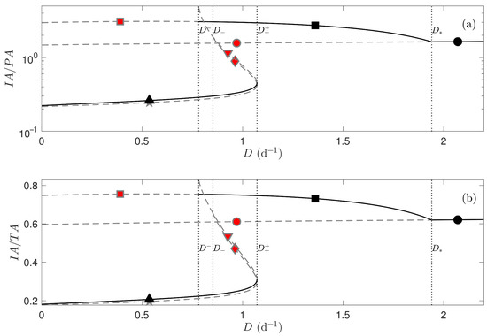
Figure 4.
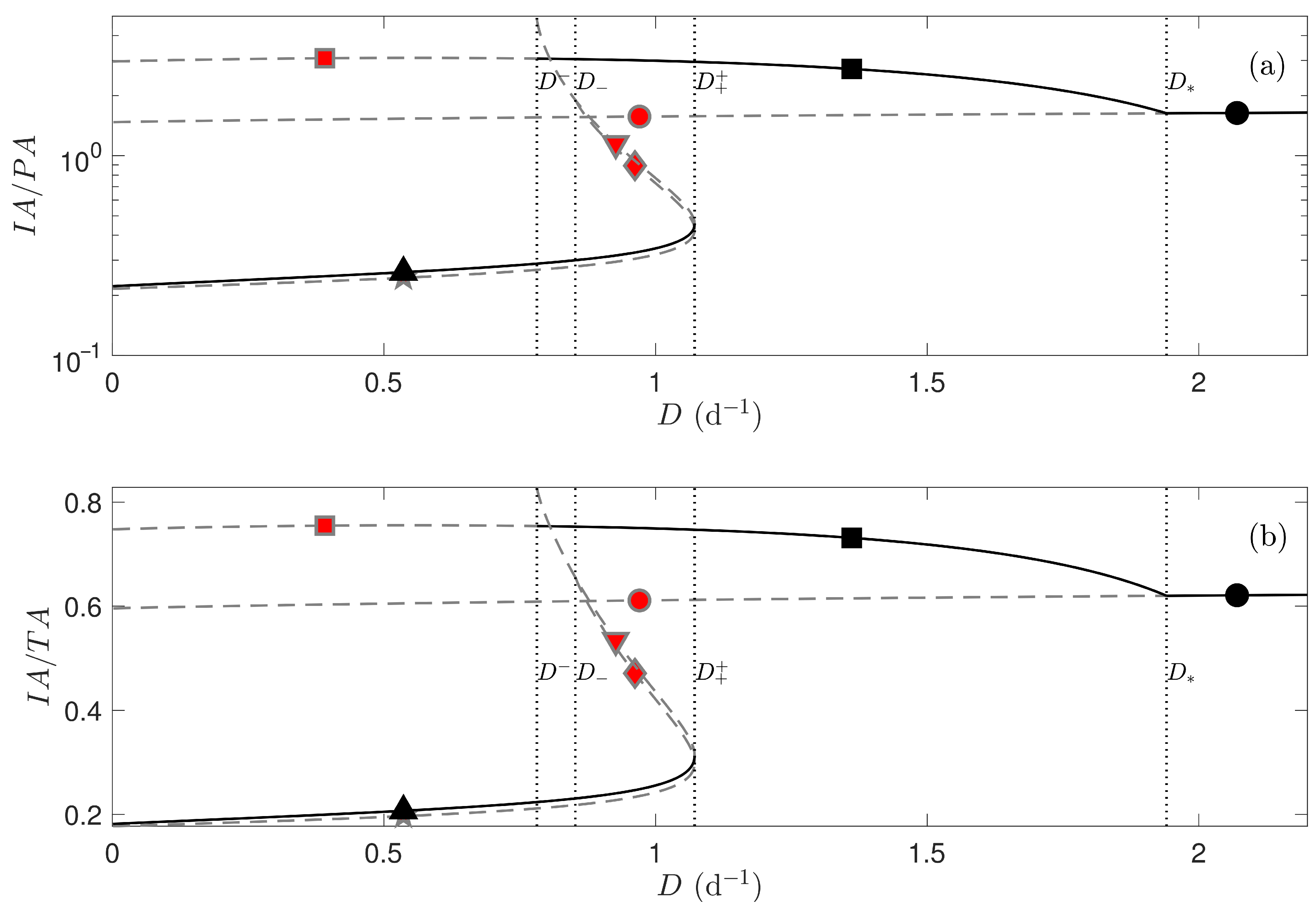
Bifurcation and stability analysis for (a) IA:AP ratio and (b) IA:AT ratio of the modified AM2 model with the parameters presented in Table 2. The continuous lines with black markers represent stable EP, the dashed lines with red markers represent unstable EP and the dotted lines are the bifurcation points, while the shape of the markers indicates the regions for each EP: ● = EP1, ▪ = EP2, ⧫ = EP3a, ★ = EP3b, ▾ = EP4a, and ▴ = EP4b.
Table 2.
Parameters for the simulation of the modified AM2 model [33]. The values of the physicochemical equilibrium constants are at standard conditions.
For the particular parameters and operating conditions (see Table 2) used to produce Figure 1, Figure 2, Figure 3 and Figure 4, there are four bifurcation points at , , , and . Notice that for this particular case , therefore, the washout of the methanogenic biomass occurs before the washout of the acidogenic biomass, as can be seen in Figure 1a,b. For the only stable equilibrium point is EP4b, i.e., with both biomasses remaining alive, while for there are two stable equilibrium points, one is EP4b and the other is EP2, i.e., both biomasses alive or only the acidogenic biomass alive, respectively. Then, for EP2 is the only stable equilibrium point and only acidogenic biomass survives and finally, for both biomasses are washed out (EP1).
Thus the anaerobic digestion process can operate correctly in , where EP4b exists and is asymptotically stable. As seen in Figure 1c,d, the stable COD and VFA concentrations approach zero for low dilution rates and increases monotonically as the dilution rate increases. In particular, as D increases, approaching , the COD concentration approaches due to the decrease of the acidogenic biomass, and for there is only one possible equilibrium point: . On the other hand, the VFA concentration has two possible stable equilibrium points for (EP4b and EP2), while for the only stable equilibrium is (EP2), because the acidogenic biomass produces more VFA and finally, for the only possible equilibrium point is (EP1). As seen in Figure 1e, the behavior of the TIC concentration is qualitatively similar to that of the VFA with respect to the number and stability of equilibrium points.
Finally, the stable equilibrium points for the pH in the system is alkaline for EP4b () and becomes acid for EP2 (), while in the washout of both biomasses () it becomes equal to the pH of the inflow (see Figure 1f). Notice that the behavior of the pH is similar to the TIC concentration.
As seen in Figure 2, the maximum methane production rate appears with a dilution rate between and , while for the methane production disappears due to the washout of the methanogenic biomass, and the flow keeps increasing due to its production associated to the acidogenic biomass and the physicochemical equilibrium that produces a desorption. Because of this, the keeps increasing even when both biomasses have been washed out.
In Figure 3, it can be observed that the behavior of the alkalinities is similar to the behavior of the VFA and the TIC. In particular, the total and partial alkalinities are qualitatively similar to the VFA concentration (compare Figure 3a,c with Figure 1d), while the intermediate alkalinity is qualitatively similar to the total inorganic carbon concentration (compare Figure 3b with Figure 1e). However, due to the behavior of the stable equilibrium points for the pH in the system (see Figure 1f), for EP4b has positive partial alkalinities (see Figure 3a). Notice that the partial alkalinity can become negative if the pH of the process is below , however, due to the parameters used here, this is not the case.
Finally, Figure 4a,b shows the behavior of the IA:PA and IA:TA ratios, respectively. An indirect regulation of the concentration of VFA will keep the system in the stable zone, since in previous studies it has been demonstrated that regulating the VFA will ensure the stability of the process [1,42] and the knowledge of the stable and unstable zones allow to propose operation paths in order to avoid process acidification, possibly leading to failure.
Ripley et al. [10] proposed that the IA/PA ratio should be IA/PA < 0.3 to have operational stability [39]. Although this criterion may seem arbitrary, it is interesting to note that this value coincides exactly with the stable operating zone , both for the IA/PA radio (Figure 4b) and for the IA/TA ratio (Figure 4b), so this criterion is fully justified for preventing acidification and the consequent system failure. Furthermore, in [1], where a pH operating range was considered and some simplifications were made accordingly, a minimum physicochemically possible ratio IA/TA was established as . In the present work, where a wide range of pH was considered, and no major simplifications were made, it was found that for (i.e., in the stable zone), minimal ratios IA/PA, and IA/TA were obtained as (Figure 4b) and (Figure 4a) respectively, which is also congruent with [1].
4.2. Predictions of an Experimental Case Study
According to Equations (31) and (32) and the electroneutrality condition given in Equation (27) it holds that
then, if , and are known, it is possible to estimate and by simultaneously solving the previous equations that are linear with respect to and to obtain:
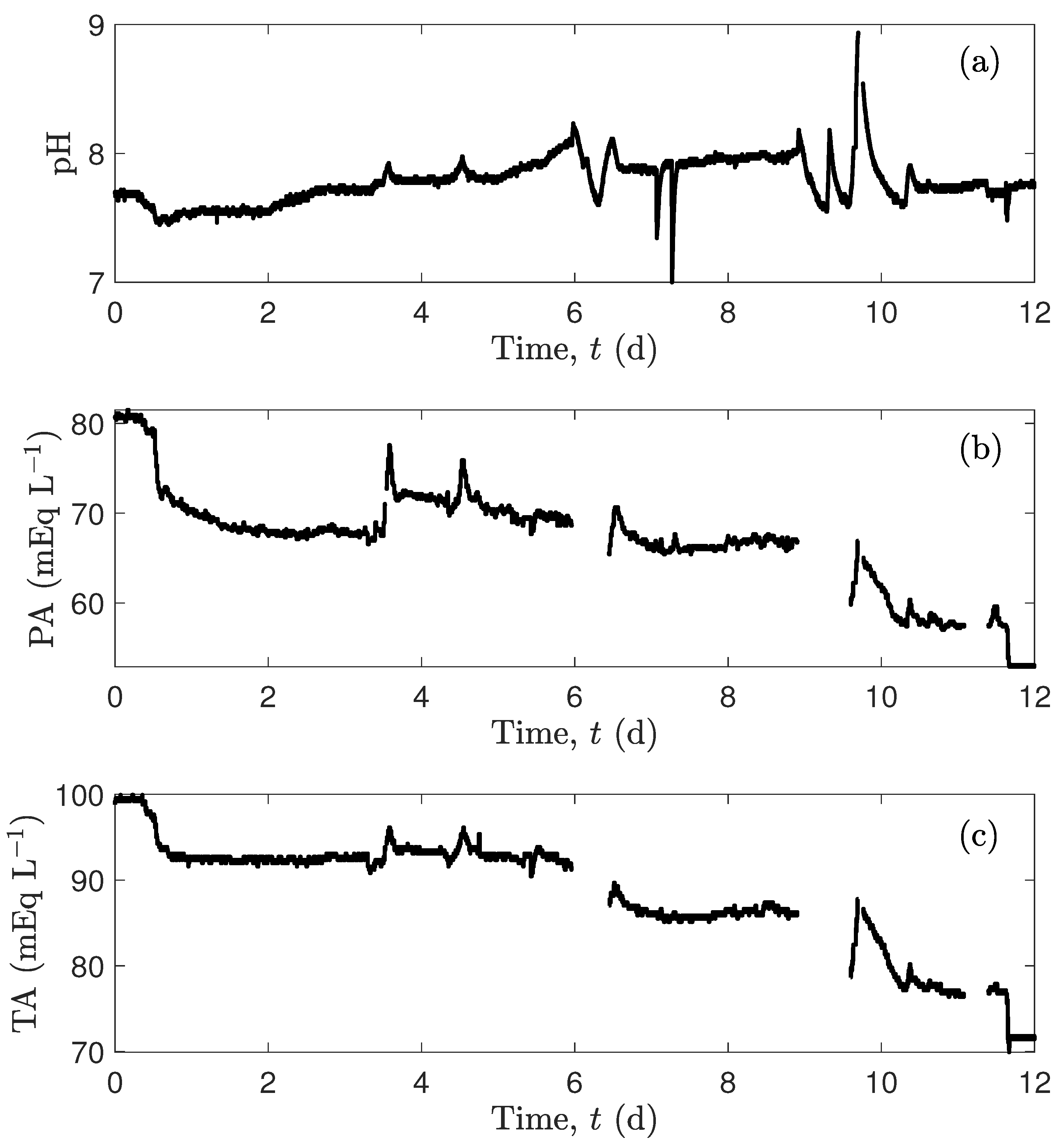
Alcaraz-González et al. [1] reported the experimental data of pH, TA, PA, VFA, and TIC in an AD process operation, carried out in an up-flow fixed-bed bioreactor for the treatment of red wine vinasses, with a useful volume of 0.982 m. For further details, see [1]. In particular, the pH, TA, and PA experimental data are presented here in Figure 5, while Figure 6 shows the VFA and CTI experimental data. Then, considering the experimental data of Figure 5, it is possible to predict the VFA and CTI concentrations with Equations (37) and (38) to validate the correlations proposed here for alkalinities using the values of , , , and reported in Table 2. However, it is important to mention that the gaps in the experimental data in Figure 5b,c and Figure 6a,b are missing data due to sensors malfunction or maintenance, mainly in the time periods 5.95 d < t < 6.5 d and 8.9 d < t < 9.6 d, nevertheless, this does not affect the validation.
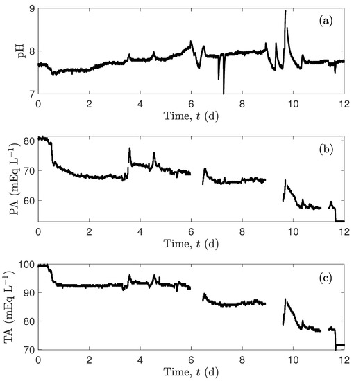
Figure 5.
Experimental data: (a) pH, (b) partial alkalinity, and (c) total alkalinity.
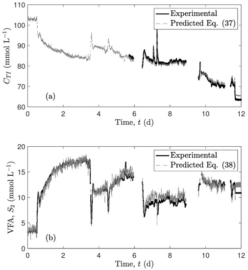
Figure 6.
Predictions of the experimental data: (a) TIC and (b) VFA.
In Figure 6a,b, the comparison of the measured variables of CTI and VFA carried out by Alcaraz-González et al. [1] and the estimation made by the proposed model are shown. Particularly, in Figure 6a it can be seen that the model performs an accurate prediction of CTI, even for abrupt changes. For instance, at approximately d the alkali input flow rate decreased, causing a decrease in the pH that also affected the CTI concentration. Something similar is also seen in Figure 6b, where an accurate prediction is also observed for the VFA concentration, with respect to the experimental data.
5. Conclusions
The proposed AM2 model reveals the interactions between the state variables and the alkalinity, bicarbonates, and acid equilibrium thanks to the inclusion of the pH behavior. The analytical and numerical roots of the proposed AM2 model shed light to all the possible scenarios of the AD process, where the process failure is identified with the death/washout of the biomass. In addition, bifurcation diagrams that were built as a function of the dilution rate provides the expected steady states while the stability analysis helps in the definition of safe operation intervals, avoiding unstable zones. Bifurcation diagrams also showed the possibility for VFA regulation, which may induce the inhibition of the methanogenic biomass through the alkalinity. Finally, a set of experimental data of the pH, the TA, and the PA of a fixed bed reactor was used to predict the values of the TIC and the VFA, both state variables of ionized species, allowing to validate the accuracy and robustness of the modified model by including the physicochemical relations of the strong ions.
Author Contributions
Conceptualization, A.C.-R. and J.P.G.-S.; methodology, A.C.-R., J.P.G.-S. and M.A.Z.-N.; software, A.C.-R., J.P.G.-S. and M.A.Z.-N.; validation, A.C.-R. and J.P.G.-S.; formal analysis, A.C.-R. and J.P.G.-S.; investigation, A.C.-R., J.P.G.-S., E.A.-G. and V.A.-G.; resources, A.C.-R. and J.P.G.-S.; data curation, A.C.-R. and J.P.G.-S.; writing—original draft preparation, A.C.-R., J.P.G.-S., E.A.-G., M.A.Z.-N. and V.A.-G.; writing—review and editing, A.C.-R., J.P.G.-S., E.A.-G., M.A.Z.-N. and V.A.-G.; visualization, J.P.G.-S.; supervision, J.P.G.-S.; project administration, J.P.G.-S. All authors have read and agreed to the published version of the manuscript.
Funding
This research received no external funding.
Acknowledgments
The authors acknowledge the grants provided by the Mexican National Council of Science and Technology (CONACyT) for its support: A.C.-R. (SNI-417882), M.A.Z.-N. (SNI-389185), V.A.-G. (SNI-25286), E.A.-G. (SNI-42019) and J.P.G.-S. (SNI-43658) through the program Sistema Nacional de Investigadores (SNI).
Conflicts of Interest
The authors declare no conflict of interest.
Abbreviations
The following abbreviations are used in this manuscript:
| AD | Anaerobic digestion |
| AM2 | Anaerobic digestion model 2 |
| AMOCO | Automatic monitoring and control project |
| COD | Chemical oxygen demand |
| VFA | Volatile fatty acids |
| PA | Partial alkalinity |
| IA | Intermediate alkalinity |
| TA | Total alkalinity |
| TIC | Total inorganic carbon |
| EP | Equilibrium point |
References
- Alcaraz-González, V.; Fregoso-Sánchez, F.A.; González-Alvarez, V.; Steyer, J.P. Multivariable robust regulation of alkalinities in continuous anaerobic digestion processes: Experimental validation. Processes 2021, 9, 1153. [Google Scholar] [CrossRef]
- Santana Junior, A.E.; Duda, R.M.; de Oliveira, R.A. Improving the energy balance of ethanol industry with methane production from vinasse and molasses in two-stage anaerobic reactors. J. Clean. Prod. 2019, 238, 117577. [Google Scholar] [CrossRef]
- Meegoda, J.N.; Li, B.; Patel, K.; Wang, L.B. A review of the processes, parameters, and optimization of anaerobic digestion. Int. J. Environ. Res. Public Health 2018, 15, 2224. [Google Scholar] [CrossRef] [PubMed] [Green Version]
- Yuan, H.; Zhu, N. Progress in inhibition mechanisms and process control of intermediates and by-products in sewage sludge anaerobic digestion. Renew. Sustain. Energy Rev. 2016, 58, 429–438. [Google Scholar] [CrossRef]
- Molino, A.; Nanna, F.; Ding, Y.; Bikson, B.; Braccio, G. Biomethane production by anaerobic digestion of organic waste. Fuel 2013, 103, 1003–1009. [Google Scholar] [CrossRef]
- Suhartini, S.; Heaven, S.; Banks, C.J. Comparison of mesophilic and thermophilic anaerobic digestion of sugar beet pulp: Performance, dewaterability and foam control. Bioresour. Technol. 2014, 152, 202–211. [Google Scholar] [CrossRef] [Green Version]
- Abbasi, T.; Tauseef, S.M.; Abbasi, S.A. A brief history of anaerobic digestion and “biogas”. In Biogas Energy; Springer Briefs in Environmental Science; Springer: New York, NY, USA, 2012; Volume 2, pp. 11–23. [Google Scholar] [CrossRef]
- Chen, Y.; Cheng, J.J.; Creamer, K.S. Inhibition of anaerobic digestion process: A review. Bioresour. Technol. 2008, 99, 4044–4064. [Google Scholar] [CrossRef]
- Chen, S.; Zhang, J.; Wang, X. Effects of alkalinity sources on the stability of anaerobic digestion from food waste. Waste Manag. Res. 2015, 33, 1033–1040. [Google Scholar] [CrossRef]
- Ripley, L.E.; Boyle, W.C.; Converse, J.C. Improved alkalimetric monitoring for anaerobic digestion of high-strength waste. J. Water Pollut. Control Fed. 1986, 58, 406–411. [Google Scholar]
- Tian, Z.; Zhang, Y.; Li, Y.; Chi, Y.; Yang, M. Rapid establishment of thermophilic anaerobic microbial community during the one-step startup of thermophilic anaerobic digestion from a mesophilic digester. Water Res. 2015, 69, 9–19. [Google Scholar] [CrossRef]
- Björnsson, L.; Mattiasson, B.; Henrysson, T. Effects of support material on the pattern of volatile fatty acid accumulation at overload in anaerobic digestion of semi-solid waste. Appl. Microbiol. Biotechnol. 1997, 47, 640–644. [Google Scholar] [CrossRef]
- Piceno-Díaz, E.R.; Ricardez-Sandoval, L.A.; Gutierrez-Limon, M.A.; Méndez-Acosta, H.O.; Puebla, H. Robust nonlinear model predictive control for two-stage anaerobic digesters. Ind. Eng. Chem. Res. 2020, 59, 22559–22572. [Google Scholar] [CrossRef]
- Sun, C.; Guo, L.; Zheng, Y.; Yu, D.; Jin, C.; Zhao, Y.; Yao, Z.; Gao, M.; She, Z. Effect of mixed primary and secondary sludge for two-stage anaerobic digestion (AD). Bioresour. Technol. 2022, 343, 126160. [Google Scholar] [CrossRef] [PubMed]
- Jiménez-Ocampo, U.E.; Santiago, S.G.; Vargas, A.; Moreno-Andrade, I. Feedback control strategy for optimizing biohydrogen production from organic solid waste in a discontinuous process. Int. J. Hydrogen Energy 2021, 46, 35831–35839. [Google Scholar] [CrossRef]
- Méndez-Acosta, H.; Campos-Rodríguez, A.; González-Álvarez, V.; García-Sandoval, J.; Snell-Castro, R.; Latrille, E. A hybrid cascade control scheme for the VFA and COD regulation in two-stage anaerobic digestion processes. Bioresour. Technol. 2016, 218, 1195–1202. [Google Scholar] [CrossRef]
- Aguilar-Garnica, E.; Dochain, D.; Alcaraz-González, V.; González-Álvarez, V. A multivariable control scheme in a two-stage anaerobic digestion system described by partial differential equations. J. Process Control 2009, 19, 1324–1332. [Google Scholar] [CrossRef]
- Hernández, M.; Rodríguez, M. Hydrogen production by anaerobic digestion of pig manure: Effect of operating conditions. Renew. Energy 2013, 53, 187–192. [Google Scholar] [CrossRef]
- Schievano, A.; D’Imporzano, G.; Adani, F. Substituting energy crops with organic wastes and agro-industrial residues for biogas production. J. Environ. Manag. 2009, 90, 2537–2541. [Google Scholar] [CrossRef]
- Parawira, W.; Read, J.; Mattiasson, B.; Björnsson, L. Energy production from agricultural residues: High methane yields in pilot-scale two-stage anaerobic digestion. Biomass Bioenergy 2008, 32, 44–50. [Google Scholar] [CrossRef]
- Moosbrugger, R.E.; Wentzel, M.C.; Ekama, G.A.; Marais, G.V. Weak acid/bases and pH control in anaerobic systems—A review. Water SA 1993, 19, 1–10. [Google Scholar]
- Palacios-Ruiz, B.; Méndez-Acosta, H.; Alcaraz-González, V.; González-Álvarez, V.; Pelayo-Ortiz, C. Modelo dinámico para un proceso de digestión anaerobia en dos etapas. In Proceedings of the XXIX Encuentro Nacional de la AMIDIQ, Puerto Vallarta, Jalisco, Mexico, 13–16 May 2008. [Google Scholar]
- Lahav, O.; Morgan, B. Titration methodologies for monitoring of anaerobic digestion in developing countries—A review. J. Chem. Technol. Biotechnol 2004, 79, 1331–1341. [Google Scholar] [CrossRef] [Green Version]
- Barampouti, E.M.P.; Mai, S.T.; Vlyssides, A.G. Dynamic Modeling of the Ratio Volatile Fatty Acids/Bicarbonate Alkalinity in a UASB Reactor for Potato Processing Wastewater Treatment. Environ. Monit. Assess. 2005, 110, 121–128. [Google Scholar] [CrossRef] [PubMed]
- Keshtkar, A.; Meyssami, B.; Abolhamd, G.; Ghaforian, H.; Khalagi Asadi, M. Mathematical modeling of non-ideal mixing continuous flow reactors for anaerobic digestion of cattle manure. Bioresour. Technol. 2003, 87, 113–124. [Google Scholar] [CrossRef]
- Saravanan, V.; Sreekrishnan, T. Modelling anaerobic biofilm reactors—A review. J. Environ. Manag. 2006, 81, 1–18. [Google Scholar] [CrossRef] [PubMed]
- Haag, J.; Vande Wouwer, A.; Queinnec, I. Macroscopic modelling and identification of an anaerobic waste treatment process. Chem. Eng. Sci. 2003, 58, 4307–4316. [Google Scholar] [CrossRef]
- Tomei, M.; Bragugloa, C.; Cento, G.; Mininni, G. Modeling of Anaerobic Digestion of Sludge. Crit. Rev. Environ. Sci. Technol. 2009, 39, 1003–1051. [Google Scholar] [CrossRef]
- Florencio, L.; Field, J.; Van Langerak, A.; Lettinga, G. pH-stability in anaerobic bioreactors treating methanolic wastewaters. Water Sci. Technol. 1996, 33, 177–184. [Google Scholar] [CrossRef]
- Liu, B.Y.; Pfeffer, J.T.; Suidan, M.T. Equilibrium Model of Anaerobic Reactors. Environ. Eng. 1995, 121, 56–65. [Google Scholar] [CrossRef]
- Bastone, D.; Keller, J.; Angelidaki, I.; Kalyuzhnyl, S.; Pavlostathis, S.; Rozzi, A.; Sanders, W.T.M.; Siegrist, H.A. The IWA anaerobic digestion model no. 1 (ADM1). Wat. Sci. Tech. 2002, 45, 65–73. [Google Scholar] [CrossRef]
- Blumensaat, F.; Keller, J. Modelling of two-stage anaerobic digestion using the IWA Anaerobic Digestion Model No. 1 (ADM1). Water Res. 2005, 39, 171–183. [Google Scholar] [CrossRef]
- Bernard, O.; Hadj-Sadok, Z.; Dochain, D.; Genovesi, A.; Steyer, J. Dynamical model development and parameter identification of an anaerobic wastewater treatment process. Biotech. Bioeng. 2001, 75, 424–438. [Google Scholar] [CrossRef] [PubMed]
- Wang, X.; Bai, X.; Li, Z.; Zhou, X.; Cheng, S.; Sun, J.; Liu, T. Evaluation of artificial neural network models for online monitoring of alkalinity in anaerobic co-digestion system. Biochem. Eng. J. 2018, 140, 85–92. [Google Scholar] [CrossRef]
- Alcaraz-González, V.; Fregoso-Sanchez, F.A.; Mendez-Acosta, H.O.; Gonzalez-Alvarez, V. Robust regulation of alkalinity in highly uncertain continuous anaerobic digestion processes. CLEAN–Soil Air Water 2013, 41, 1157–1164. [Google Scholar] [CrossRef]
- Benyahia, B.; Sari, T.; Cherki, B.; Harmand, J. Bifurcation and stability analysis of a two step model for monitoring anaerobic digestion processes. J. Process Control 2012, 22, 1008–1019. [Google Scholar] [CrossRef] [Green Version]
- Hess, J.; Bernard, O. Design and study of a risk management criterion for an unstable anaerobic wastewater treatment process. J. Process Control 2008, 18, 71–79. [Google Scholar] [CrossRef]
- Shen, S.; Premier, G.C.; Guwy, A.; Dinsdale, R. Bifurcation and stability analysis of an anaerobic digestion model. Nonlinear Dyn. 2007, 48, 391–408. [Google Scholar] [CrossRef]
- Méndez-Acosta, H.; Palacios-Ruiz, B.; Alcaraz-González, V.; González-Álvarez, V.; García-Sandoval, J. A robust control scheme to improve the stability of anaerobic digestion processes. J. Process Control 2010, 20, 375–383. [Google Scholar] [CrossRef]
- Seydel, R. Practical Bifurcation and Stability Analysis. In Interdisciplinary Applied Mathematics; Springer: New York, NY, USA, 2009; Volume 5. [Google Scholar] [CrossRef]
- Harris, D.C. Quantitative Chemical Analysis; Macmillan: New York, NY, USA, 1995. [Google Scholar]
- Schaum, A.; Alvarez, J.; Garcia-Sandoval, J.P.; Gonzalez-Alvarez, V.M. On the dynamics and control of a class of continuous digesters. J. Process Control 2015, 34, 82–96. [Google Scholar] [CrossRef]

Publisher’s Note: MDPI stays neutral with regard to jurisdictional claims in published maps and institutional affiliations. |
© 2022 by the authors. Licensee MDPI, Basel, Switzerland. This article is an open access article distributed under the terms and conditions of the Creative Commons Attribution (CC BY) license (https://creativecommons.org/licenses/by/4.0/).