1. Introduction
Historically, floods in Canada occur in the spring, due to snowmelt, and in the summer, due to intense thunderstorms [
1,
2,
3]. Urbanization has amplified the flood risks due to rapid runoff from impervious surfaces. Floods jeopardize lives, and inundation-prone areas suffer devastating economic losses. In this context, governments rely on early flood warning and forecasting systems to help protect lives and prevent property damage by deploying countermeasures [
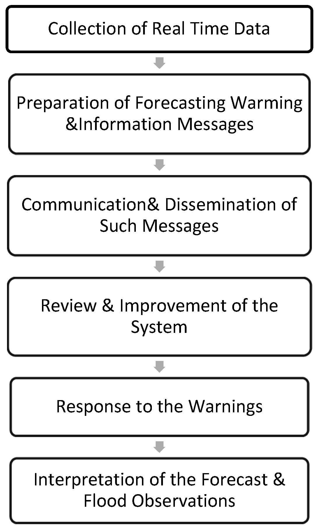
4]. The flow chart in
Figure 1 illustrates a typical flood warning system.
Compared to traditional solutions, which assess flood risks, early flood forecasting and warning systems play a more significant role in alerting people of imminent floods [
5,
6]. Early flood warning systems usually come with different lead times, which play a critical factor in the control and mitigation of risks during a flood hazard and related disasters. Such multi-functional forecasting systems enhance community preparedness in the context of floods and minimize losses that usually follow a flood. The system will typically predict the scale, timing, location, and likely damages of the flood [
7]. It draws data all year round from sensors placed in strategic points of the water basins, such as in lakes and rivers, or on flood defenses such as dams, dikes, embankments, or specially constructed structures for flood forecasting and monitoring. Promising preventive measures require extensive collaboration across multiple disciplines, such as deep learning algorithms, remote sensing, hydrology, and meteorology [
8,
9]. Forecasting model integrity is enhanced due to the collaboration of such disciplines. These forecast models are developed and managed by assessing flood risks, local hazard monitoring, flood risk dissemination services, and community response [
10].
It is common for countries to deploy large-scale sensor networks, given the flood dis-asters previously faced [
11]. Large-scale sensor networks collect critical data on water bodies, such as water velocity, temperature flooding, etc. The growing availability of such data, combined with the need to prepare for flood situations, has pushed researchers to analyze how existing computational resources can improve forecast accuracy. The popularity of deep learning and machine learning technologies enables the transformation of practical knowledge into actionable ones. “Emerging advances in computing technologies, coupled with big-data mining, have boosted data-driven applications, among which Machine Learning (ML) technologies bearing flexibility and scalability in pattern extraction has modernized scientific thinking and predictive applications” [
12]. Technologies with deep learning, big-data mining, aggregation, and model ensemble drive methodologically oriented countermeasures that aid in forecasting certain hydrological parameters. The parameters included are reservoir inflow, reservoir inflow, river flow parameters, tropical cyclone tracking, and anticipating different lead times in flooding.
Deep learning is a subset of machine learning, which employs multiple layers of neural networks that can gain knowledge and acquire skills akin to the working of the human brain [
13,
14]. The proliferation of deep learning algorithms has given rise to an improvement in deep learning capabilities. The popularity of deep learning, for forecasting, stems from the fact that data, in the real world, evolve with time and are represented as time-series problems [
15]. These are highly diverse, unstructured, inter-connected, and contain spatio-temporal patterns. Deep neural networks can handle complex time series better, offering robust computational facilities in the form of advanced data processing, reduced complexity in data processing, and improved accuracy in model prediction [
16].
Physical hydrological models, such as the Environmental Protection Agency Storm Water Management Model (EPA-SWMM) were developed to simulate flooding events in cities. Still, these models are not available for older and larger megacities due to the SWMM relay to the high precision mapping and a simulation of the underground drainage system [
17]. Then, the semi-physical hydrological models, such as the Cellular Automata (CA), need correlation calculation and an abundance of analysis for the datasets [
18]. This way, researchers combine the rainfall-runoff model and a flood-level map database to improve the alert system. They can momentarily estimate the spatial distribution of flood depth by engaging GIS tools in the flood area [
19,
20,
21]. There are no solutions for the spatial depth measurement of rainstorm events. Therefore, our research focus is on improving the performance of hybrid Long Short-Term Memory (LSTM) hydrological models.
Missing values or corrupt values typically cause a lack of uniformity in a normal situation. Still, in the case of flood forecasting, the lack of uniformity is caused by sporadically available data and at either increasing or decreasing time-space intervals [
22]. This makes prediction accuracy a problem in flood forecasting. Such sporadic data with time-series problems are also present in many forecasting and prediction areas. The deep neural network contains the required structure to control the complexity, especially CNN. Many scientific domains benefit from a wealth of satellite and model output data because huge amount of data are needed to fit [
23]. Spatio-temporal data and time-series problems are huge challenges for space technology developments [
16,
24,
25]. Spatio-temporal data, characterized by complex information and heterogeneous aspects, can create uncertainties where a network topology might not scale [
26,
27].
The spatio-temporal nature of data is perhaps the biggest challenge when it comes to flood forecasting with CNN and LSTM. Spatio-temporal data has three dimensions: the two-dimensional spatial and the temporal dimension [
28]. In the quantitative analysis end, collected time-series data may be used to capture geographical processes, such as in flood forecasting systems, at some defined regular interval [
29,
30]. It might also happen at irregular intervals, such as in the case of continuous daily occurrences or discrete occurrences, as to when an event might occur randomly in the temporal scale [
31].
Spatio-temporal data is not that easy to access, nor is it smooth. It has both local correlations, as well as gradients. In addition, there are spatio-temporal mutations. “As the accumulation of spatio-temporal data, the low-quality problems of multivariate spatio-temporal data become clear and mainly present numerous missing data, high noise of time series and great different spatial scale of spatiotemporal data” [
29,
30]. Therefore, spatio-temporal data preprocessing can help improve prediction accuracy.
Artificial Neural Network (ANN) refers to a complex network structure formed by many interconnected processing units (neurons) [
32,
33]. A form of ANN called the Recurrent Neural Network (RNN) is used frequently in forecasting. RNN has arbitrary connections between the neurons, and the recurrent connections allow memory to be persisted in the internal state. Unlike an ANN, the independent layers in RNN are converted to the dependent layer [
34]. The same bias and weight are used. All hidden layers are joined up as a single recurrent layer. This enables the RNN to process inputs of any given length. As more layers are added using specific activation functions, the gradients of the loss function approach zero, which makes the network hard to train [
35]. This is inevitable, as some activation functions, such as the sigmoid, for instance, will manage large input spaces in smaller input spaces, and this will change the output. In turn, the derivative becomes smaller and, over time, will exponentially decay. The learning of long-term data sequences is, therefore, hampered. As the gradient that carries information in RNN becomes smaller and the parameter updates to new inputs become negligible, there is no real learning. Therefore, the forecasting benefits of RNN are hindered. A solution to this vanishing gradient problem in RNN is the LSTM networks [
36].
LSTM is an improvement over simple RNN, which captures sequential data long-term dependence [
37,
38,
39]. The LSTM architecture includes specially designed gates, units, and memory cells [
40,
41,
42] that learn and retain the state of information, while deciding when to forget irrelevant data [
43]. Simple RNNs, in comparison, only update a single past state. The cell state, serving as the system’s memory, restores the system’s capability through backpropagation and time algorithms [
44,
45].
LSTM models employ these neuron gates to learn, forget, and surround cell memory for better control of information flow. With training, the input gate becomes proficient as a control for the input that must be remembered for a certain period [
45].
Advanced deep learning methods, such as Convolutional Neural Network (CNN) and LSTM, offer a better spatio-temporal series prediction than a simple time series prediction, for the extraction of abstract and high-level information, from images and complex data [
46]. ConvLSTM is a variant of LSTM in that it has the convolution operation inside the LSTM cell. On the other hand, both models are special types of RNN and have deep learning capabilities [
47,
48]. ConvLSTM replaces the matrix multiplication operation at the gates, to better capture underlying spatial features with convolution, and varies from LSTM based on the input dimensions. It is specifically designed for 3D data. CNNLSTM is an integration of CNN with LSTM. As such, the CNN model is specifically integrated with LSTM, allowing the CNN model to process data and then use LSTM for processing the one-dimensional result feed, since LSTM cannot process multiple dimensions.
Contributions
The spatio-temporal attention LSTM model combines the LSTM structure and spa-tio-temporal attention module to selectively use the critical and useful hydrological features [
43]. For the spatio-temporal attention LSTM model (STA-LSTM), the main LSTM network is used for feature extraction, temporal correlation, and final classification. The temporal attention is used to assign appropriate importance to different frames, and the spatial attention is used to assign appropriate priority to other nodes [
49].
Almost all researchers’ hydrological predictions employ a single monitoring station, producing a time-series prediction. However, rivers contain many monitoring stations, where adjacent monitoring stations’ discharge values correlate. Flood forecasting is a spatio-temporal prediction problem. One should build the relationship between the upstream monitoring stations and the downstream monitoring stations that is important to improve the accuracy of flood prediction when an earlier warning is needed. Urban flood prediction is the beginning of flood forecasting. We find the most important factors to be the discharge of upstream monitoring stations and precipitation for the hybrid models [
50]. Due to complex spatio-temporal datasets and high accuracy, the system needs more efficient models.
Therefore, our research aims to expand the time series prediction to include spatial information to improve forecasting. To achieve this objective, this research adopted modified hybrid LSTM variations [
51], such as Convolutional Neural Networks LSTM model (CNN-LSTM), Convolutional LSTM model (ConvLSTM), and Spatio-temporal Attention LSTM model (STA-LSTM) [
43].
2. Materials and Methods
2.1. Study Area and Materials
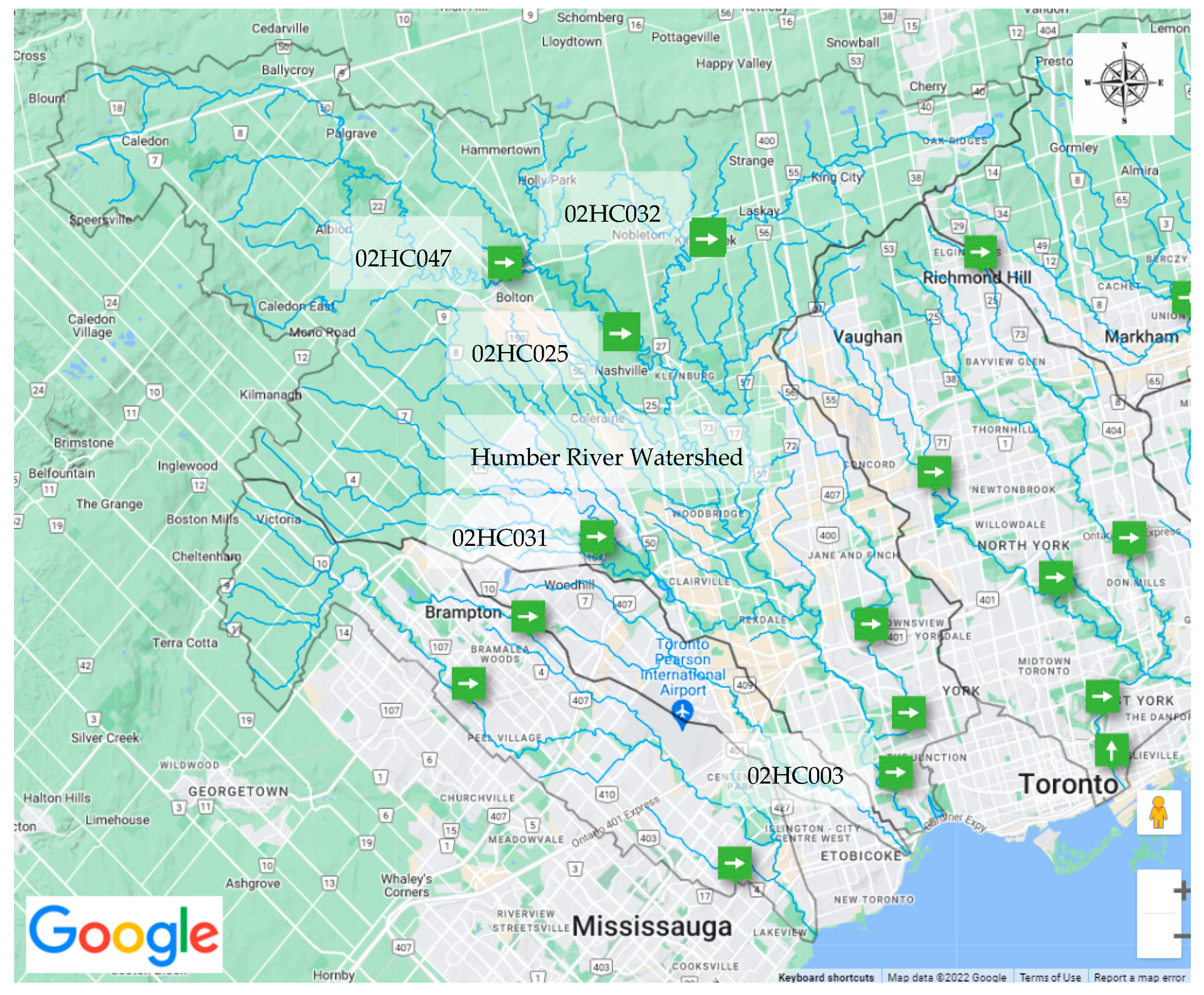
The Humber River is one of the most important rivers in Southern Ontario, Canada. It is a tributary of Lake Ontario, and it is one of two major rivers on either side of the city of Toronto. The flood forecasting of the Humber River greatly influences the western parts of metropolitan Toronto. Humber River’s Station 02HC003 is the nearest to Toronto, making it a key piece in the flood forecasting for this metropolitan area.
The Humber River flows right through downtown Toronto, so the discharge prediction of the south of Humber River will be crucial to protecting human life and property. The network of real-time tipping-bucket rainfall monitoring in the Humber River watershed is sparse and does not accurately capture the spatial variability of the intense, localized summer thunderstorms. Therefore, the raw rainfall data must, first, be pre-processed and accumulated for the watershed, over time and space, before it can provide meaningful input to the machine learning model. Therefore, to keep the flood forecasting system simple and practical, yet fairly accurate, we decided not to include rainfall monitoring data as part of the scope of this manuscript.
Moreover, the perfect early flood forecasting system could better coordinate the interests of the government, the affected people, and the insurance industry in the sharing of flood losses. Due to the trend of insured catastrophic losses increasing year by year, the high accuracy early flood forecasting system should be accessible to everyone immediately.
From
Figure 2, we can identify that Stations 02HC025, 02HC031, 02HC032, and 02HC047 are in the headwaters of the Humber River Watershed and upstream of the critical station 02HC003 which is located in the flood-prone areas of downtown Toronto near the mouth of the Humber River watershed.
The hydrological prediction models perform well on the time series data, so they were evaluated for the spatio-temporal data. Since the STA-LSTM has a good performance on the flood prediction with time-series data, we will compare the performance of the CNN-LSTM model, ConvLSTM model, and STA-LSTM with the spatio-temporal data for flood forecasting. We applied LSTM based models because they are highly capable of dealing with spatio-temporal series-based data sequences as compared to traditional models (e.g., M5MT, extreme learning machine (ELM), SVM) [
52]. These models are based on automatic feature learning and consider the previous information during training.
Due to the level of urbanization and size of the Humber River watershed, the catchment response time typically ranges from 5 to 10 h, depending on the rainfall storm event type and duration (e.g., short-burst but intense summer thunder storms versus longer duration rainfall combined with snowmelt events in the spring). The Flood warnings for the Humber River watershed must be issued to a range of users and for various purposes. These purposes may include: readying operational teams and emergency personnel, warning the public of the timing and location of the event, and in extreme cases, to enable preparation for undertaking evacuation and emergency procedures. Therefore, we train/test the model for 12-h-ahead and 24-h-ahead forecast scenarios and evaluate model accuracy.
2.2. Datasets and Data Preprocessing
Six years of hourly dataset from five stations will be used, provided by stations 02HC047, 02HC032, 02HC031, 02HC025, and 02HC003. The five stations are located in the west of Toronto. We would predict the discharge (unit: m3/s) of station 02HC003, which is in the flood-prone areas of Toronto, and we will observe the mean square error (MSE) and mean absolute error (MAE) to evaluate the forecasting performance.
We selected 70 percent of the dataset for training, covering the period from 2012 to 2014. The following 20 percent of the data is used for testing, covering the period from 2016 to 2017. The remaining 10 percent of the data is reserved for validation, covering the 2015 year. We used five stations to test the four kinds of hybrid LSTM models and compare their mean square error. We evaluated forecasts from 1-h ahead to 12-h ahead, employing the past 24-h monitoring as input.
2.3. Models
The LSTM, ConvLSTM, and CNN-LSTM models were implemented in TensorFlow, using Keras library in Python, and the STA-LSTM was implemented in torch.nn by using the nn.Module in Python. A batch size of 50 and 200 epochs has been used in the research because the optimal epochs could prevent the model from overfitting or underfitting.
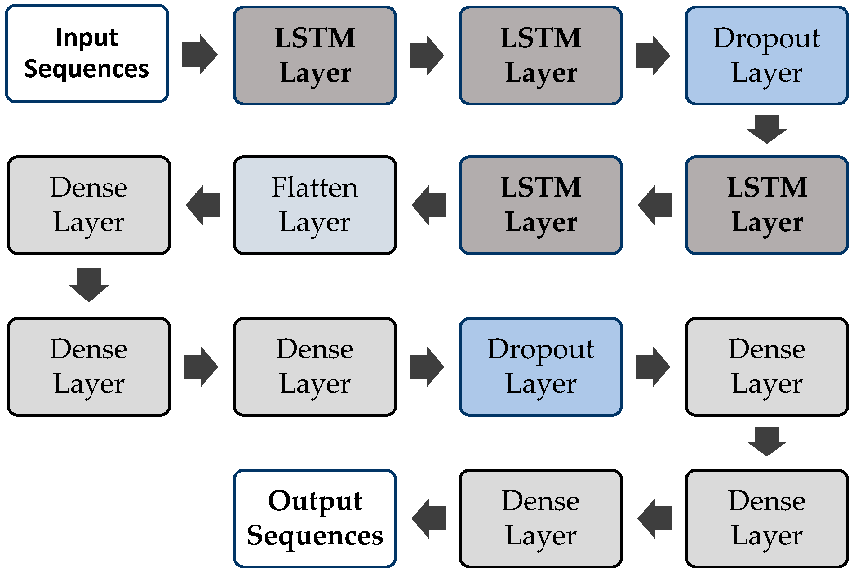
A LSTM is a neural network that accounts for dependencies in a spatio-temporal series, which is commonly used for forecasting purposes. The altering of flood forecasting is from a time series prediction to a spatio-temporal series prediction. The LSTM model is a good choice for the beginning. The structure of the LSTM model is presented in
Figure 3, which is comprised of LSTM layers. In the structure, input sequences are provided to the input layer followed by two LSTM layers. The dropout layer is added to prevent the model from overfitting, and then, two LSTM layers are added, followed by a Flatten layer. Three dense layers are added, followed by one dropout and three dense layers, which are used to change the dimensions of the vectors. Finally, the last output layer returns the output sequences. The equations of each layer of the LSTM model are given as:
where
represents the input gate,
represents the output gate,
represents the forget gate,
represents the memory cell,
represents a hidden state,
and
represent the inputs of previous timestamps,
denotes the current timestamp,
symbolizes the sigmoid function,
represents the bias of respective gates, and
represents the weights of respective gates.
ConvLSTM is a repetitive neural network for spatial-temporal prediction with state-of-the-art, state-to-state, and phase-to-phase convolutional characteristics.
Figure 4 shows the structure of a ConvLSTM model. ConvLSTM predicts the future state of a grid cell based on the income and historical status of its neighbors [
53,
54]. The ConvLSTM can keep the input features as three-dimensional (3D), and it still reserves the advantages of Fully Connected-LSTM [
55]. In this study, we used a ConvLSTM model with two convolutional layers and LSTM layers. After providing the sequences of the input layer, two convolutional layers are added, followed by one dropout layer, to avoid the overfitting. Preceding this, two LSTM layers are added to make the ConvLSTM model followed by a flatten layer. Six dense layers are added to the model, and a dropout layer is added in the middle. The output layer provided the output sequences [
55].
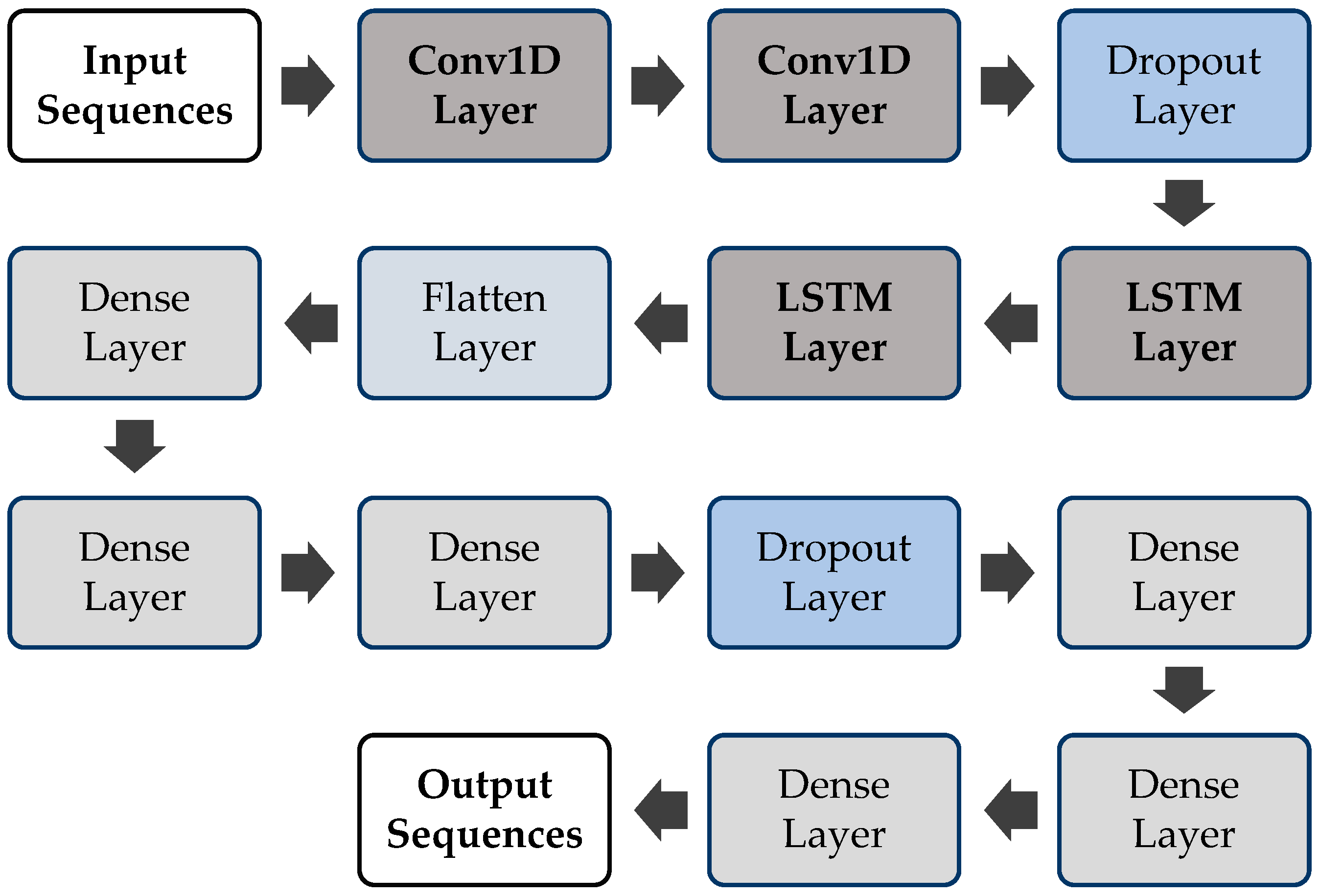
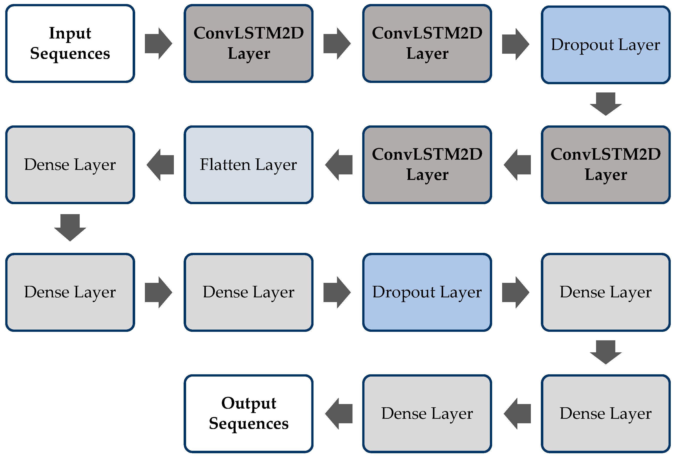
CNN-LSTM was initially known as a Long-term Recurrent Convolutional Network (LRCN) model, but in this article, we will use the most common term, “CNN-LSTM”, to refer to LSTMs that employs a CNN as a front end [
56]. The LSTM model can process the dataset of CNN and the LSTM sequences that come from the one-dimensional result of CNN. The structure of a CNN-LSTM model used in this study is shown in
Figure 5. We used four CNN-LSTM layers with a combination of other layers, including dropout, flatten, and dense layers. Two ConvLSTM2D layers are added followed by a dropout layer, and then, two more ConvLSTM2D layers are included. The remaining setup of layers is similar to the previously discussed models.
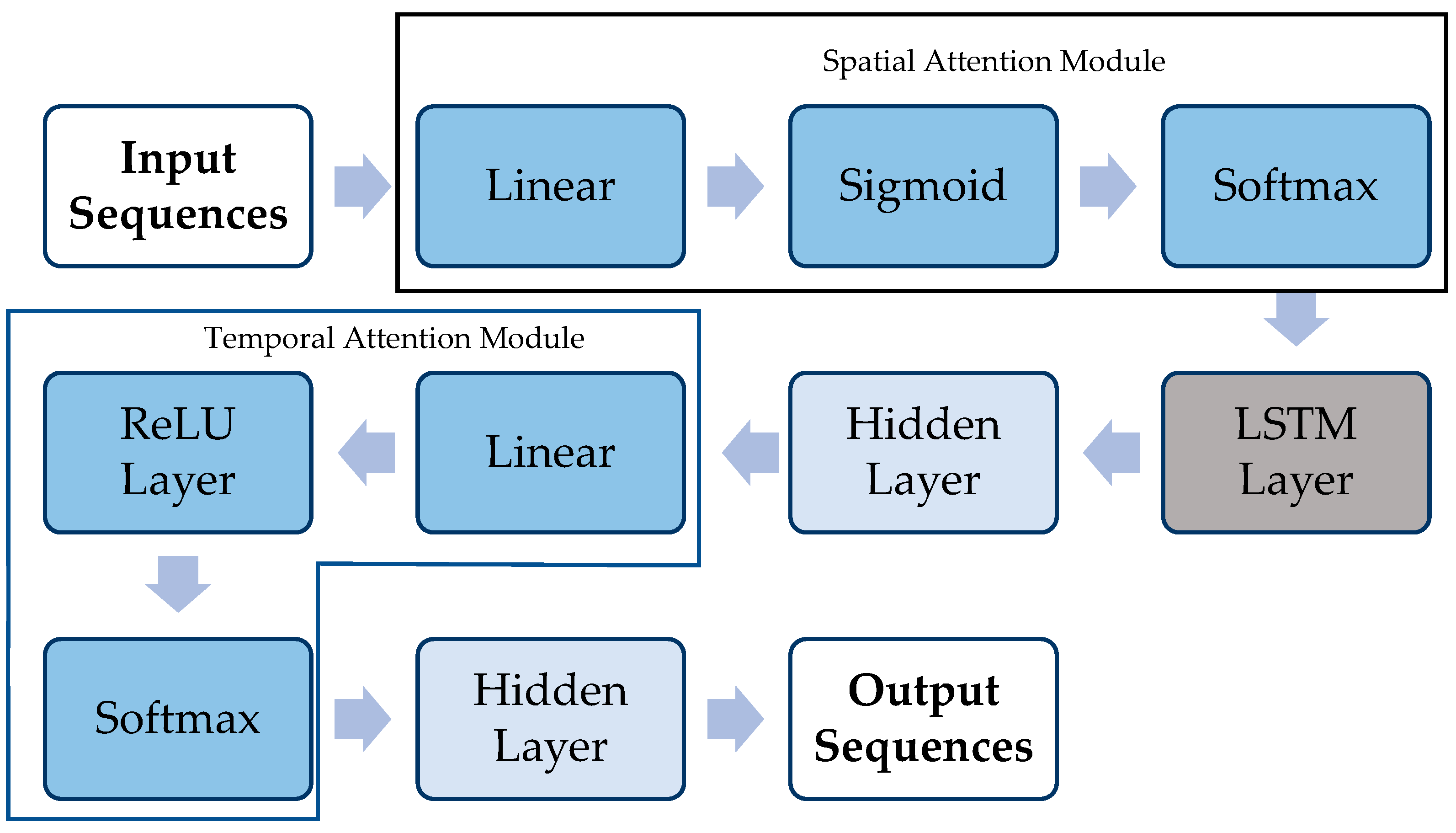
The STA-LSTM is the spatial attention operation and the temporal attention operation introduced into the LSTM cell to make full use of the spatio-temporal information of the input. The spatial attention operation works for the input features and the temporal attention operation works with the hidden layer of the LSTM. Therefore, the spatial attention weights and the temporal attention weights affect the inputs and the output, respectively [
43]. Debugging the Spatial attention weights and the temporal attention weights is the main method to improve the performance of the STA-LSTM model.
Figure 6 shows the structure of an STA-LSTM model developed in this study. The input sequences are provided to the spatial attention module, which is comprised of three layers, including linear, sigmoid, and softmax layers. After that, the LSTM layer is added, followed by the hidden layer, and passed the information to the temporal attention module, which consists of linear, ReLu, and softmax activation functions.
2.4. Evaluation Measures
Three evaluation measures are used to evaluate the performance of proposed models. Each evaluation functions are described below:
The Mean Square Error function is defined as:
where
is the total number of data points,
is the observed value, and
is the predicate value.
We also use Mean Absolute Error (
), defined in (8), to evaluate the purposed model’s performance because there are some outliers for each station that measures flood season. The meaning of the same symbols is the same as that in the
MSE. It is well known that the median is more robust than the mean for outliers, so
is more stable for outliers than
.
The
is used as the third evaluation measure concept. We could intuitively find the proximity of predictions and the observations by the error rate. When the error rate is smaller, the forecasting accuracy is higher.
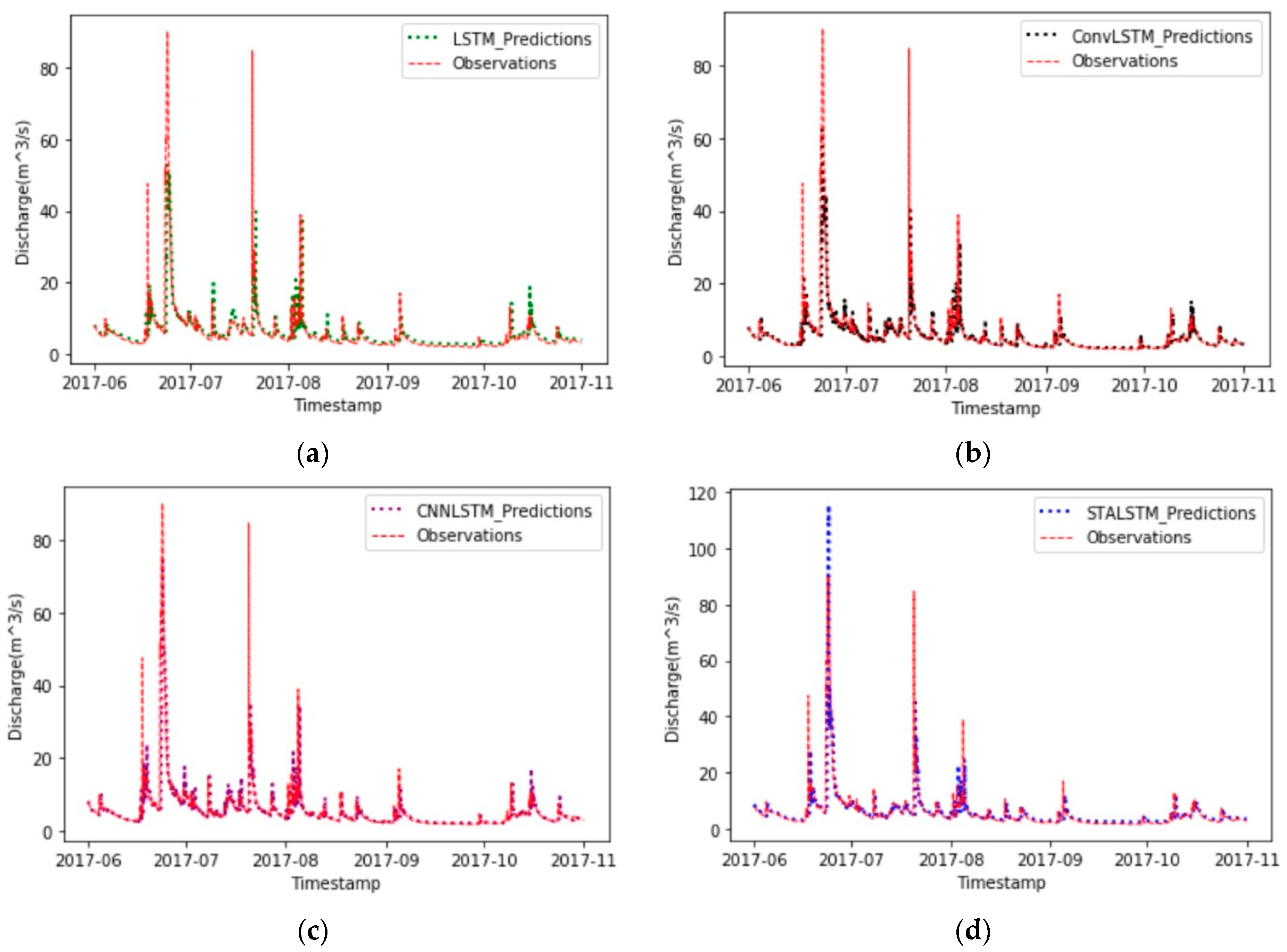
3. Results
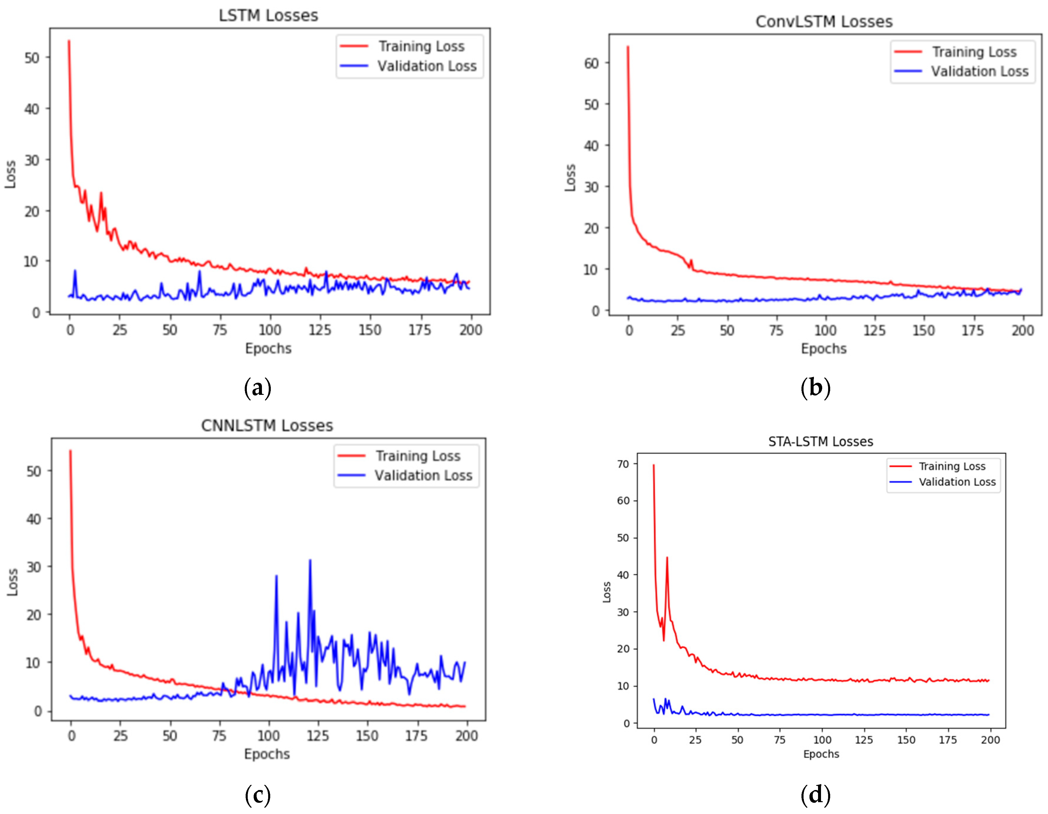
Due to the transformation of the dataset from the time series to a spatial-temporal series, as well as the deficiency of precipitation around the Humber River, we use the dataset from five different stations near each other. According to the
MSE, the training error and validation error by 12 h-ahead for the LSTM model, ConvLSTM model, CNN-LSTM model, and STA-LSTM model are plotted in
Figure 7.
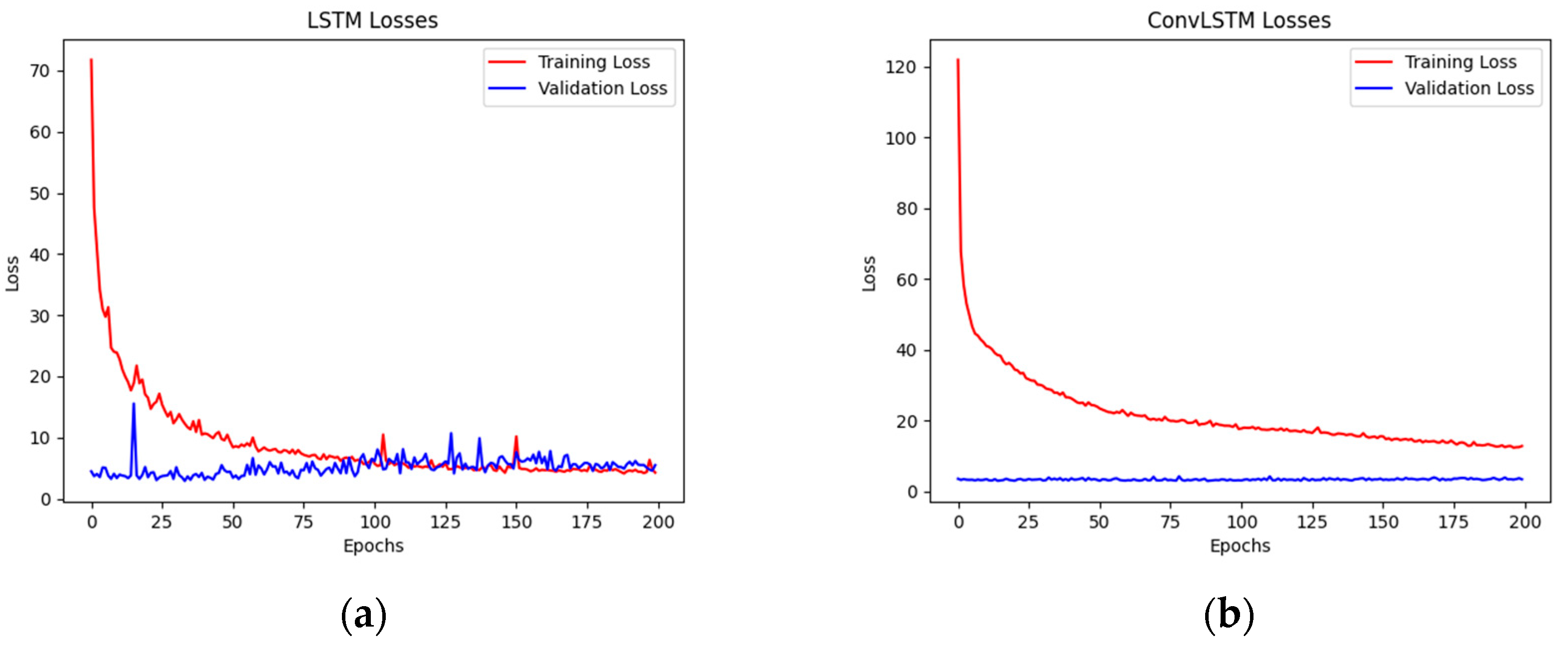
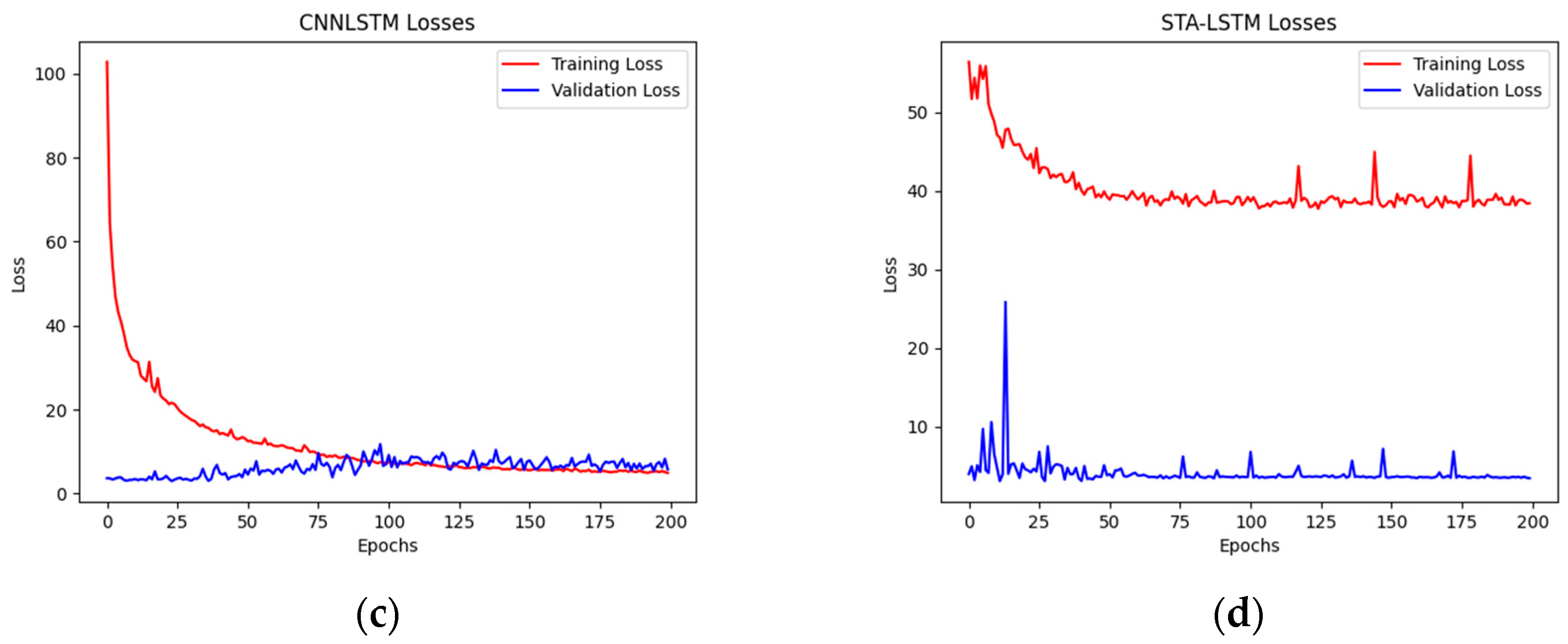
By building a longer forecasting time, residents in flood risk areas will have adequate time to evacuate, ensuring the highest degree of safety. Preceding this, the 24 h-ahead forecasting model is run to determine the training and validation error. The training and validation error for the 24 h-ahead LSTM model, ConvLSTM model, CNN-LSTM model, and STA-LSTM model are given in
Figure 8.
Comparing the variation trend training loss and validation loss, we can judge the learning state of the model and the problems of a dataset. Then, we change the quantity and size of layers to improve the performance of the models. Additionally, we list the MSE and MAE for each hour ahead.
Table 1,
Table 2 and
Table 3 show the results of
MSE,
MAE, and the error rate, respectively. When the forecasting time increases, the
MSE,
MAE, and error rate also increases. However, the STA-LSTM model has the better performance because the
MSE,
MAE, and error rate of 24 h-ahead forecasting are the lowest, as shown with the red value.
We find that the
MSE,
MAE, and ER are not sufficient to prove model performance, so we use the Fisher test (F-test) to confirm that the performance of the STA-LSTM model is better than the other three. For the aim, the F-test applies the
F-
ratio (
criterion. An F-test is a statistical analysis test, built within a certain confidence interval, to help distinguish the accuracy of the model prediction. The test takes into account the experimental and model uncertainties to evaluate the performance of the models. To perform the F-test analysis, a significance level and
value must be computed. The status of the hypotheses can either be accepted or denied based on the
value that is defined as
A higher
value indicates a more suitable model [
57]. The
is given in
Table 1, and the mean square regression (
) is defined as
where
is the
i-th prediction value,
is the
i-th observation,
is the mean of
,
is the number of data samples, and
is the number of input variables.
Then we get the
as given in
Table 4.
Although all the proposed models are accepted by the , the of the STA-LSTM model is better than the other three.
Furthermore, we use the uncertainty and reliability to control the accuracy level of the under-study models in a certain domain [
58]. An uncertainty analysis is performed to restrict the true value of an experimental outcome. The uncertainty interval is given as:
where
is the sample average,
is 1.960, and
is the sample standard deviation. This can be completed using an uncertainty interval of U95, meaning 95 out of 100 experiments completed will lie within the given interval [
58]. The equation is:
In the four flood forecasting proposed models, the STA-LSTM model had the lowest uncertainty value (
) when the forecasting time is 24 h-ahead, while the LSTM model (
) is the highest value of uncertainty in
Table 5. Therefore, in terms of U95, the STA-LSTM model outperformed the other three hybrid LSTM models. Then, a reliability analysis was conducted to statistically determine the overall model consistency. The two equations used in the analysis are as follows:
If the relative average error (RAE) is less than the threshold value of an adequate water quality parameter, the
, meaning the ki is the amount that the RAE is less than or equal to the water quality parameter [
59]. The optimum value is 0.2, according to the Chinese Standards.
From
Table 6, it is conspicuous that the STA-LSTM model, with
, was the most reliable model of the four proposed models when the forecasting times are 12 h-ahead and 24 h-ahead.
5. Conclusions
Forecast accuracy concerning the magnitude and the timing of the flood water levels diminishes significantly with forecast time, which is a critical aspect of an early warning system. Only models that can accurately predict flood water levels with sufficient warning time to allow safe evacuation can be useful tools. Our work has advanced flood forecasting accuracy, using spatio-temporal tools and deep learning algorithms to utilize the newly established real-time river monitoring network.
The new models presented here will be helpful for governments, insurance companies, local authorities, and first respondents to manage major flood events effectively. This study focused on summer thunderstorm events that are the dominant process for urban areas such as the city of Toronto. The STA-LSTM model has better performance for the summer thunderstorm events, as shown by the forecasting lowest error rate at about 3.98% for a 12-h-ahead prediction.
Almost all floods from extreme climate, such as torrential rain and global warming (snowmelt, ice jam, etc.), would require building the spatio-temporal relationship between the flow, the air temperature, the precipitation, and the snow depth. Therefore, for future work, we will face complex dataset pre-processing, such as normalization, due to the different units. We plan to test and compare the STA-LSTM model and the Spatio-temporal Attention Gated Recurrent Unit (STA-GRU) model, as well as the Generative Adversarial Networks Long Short-term Memory (GAN-LSTM) model. Including GAN models might help accuracy as the spatio-temporal dataset sizes increase. We will add more features, such as snow depth surveys, air temperature, and precipitation, as model inputs to improve the spring snowmelt floods’ accuracy, which are the dominant process in rural watersheds in Canada.


 and
and 


