Abstract
Suspended sediment yield (SSY) prediction plays a crucial role in the planning of water resource management and design. Accurate sediment prediction using conventional models is very difficult due to many complex processes. We developed a fully automatic highly generalized accurate and robust artificial intelligence models for SSY prediction in Godavari River Basin, India. The genetic algorithm (GA), hybridized with an artificial neural network (ANN) (GA-ANN), is a suitable artificial intelligence model for SSY prediction. The GA is used to concurrently optimize all ANN’s parameters. The GA-ANN was developed using daily water discharge, with water level as the input data to estimate the daily SSY at Polavaram, which is the farthest gauging station in the downstream of the Godavari River Basin. The performances of the GA-ANN model were evaluated by comparing with ANN, sediment rating curve (SRC) and multiple linear regression (MLR) models. It is observed that the GA-ANN contains the highest correlation coefficient (0.927) and lowest root mean square error (0.053) along with lowest biased (0.020) values among all the comparative models. The GA-ANN model is the most suitable substitute over traditional models for SSY prediction. The hybrid GA-ANN can be recommended for estimating the SSY due to comparatively superior performance and simplicity of applications.
1. Introduction
Sediment load is one of the most significant of nature’s landscape transformation processes on Earth and is a result of weathering. Rivers contain the sediment and transport the weathered materials of continents into the ocean. Rivers are the most important dynamic geological transportation media on the earth and serve as a vital link between the land and the ocean. Sediment movement in a river is a complicated nonlinear phenomena that involves the interaction of components of hydrology and geology with geographical and temporal variations. The accurate estimation of a river’s carried sediment load is critical for the management, planning and project management of water resources [1]. It is also necessary for information on a variety of river improvement and utilization issues [2]. The sediment load in river basin system can influence dam filling, safety of fish and wildlife habitats, water pollution, understanding of flood volume and life of hydroelectric equipment etc. [3,4,5,6,7,8,9]. The harmful effects of suspended sediment yield (SSY) in a river system and the need to understand SSY behavior has drawn substantial attention over recent decades. Dam failure is possible as a result of loss of storage capacity caused by sedimentation [10,11], where the dam’s effectiveness, built for flood control, irrigation and power generation, decreases due to sedimentation. Sediment load can also impair navigation channels, the capacity of roadside streams, rivers and ditches to move sediment, and the storage capacity of lakes and reservoirs resulting in an increased frequency of flooding [12]. Many people are affected and can lose their properties as a result of such flooding. Various studies regarding flooding due to high sedimentation and its harmful impacts have also been undertaken by many researchers [13,14].
Over the past few decades, the necessity to ensure the correct modelling of SSY has increased rapidly. However, sediment estimation is not an easy task because of its non-linear nature and complex processes in sedimentations. Quantitative estimation of SSY is quite tough either manually, or by means of instrument for automated sampling, which both involve more labor demanding, time consuming and costly procedures [15,16]. Due to the incidence of multiple complex procedures, determination of sediment data is not very accurate with traditional methods. A conventional multiple linear regression (MLR) regression approach has been utilized for the prediction of SSY [17,18,19]. However, this model can capture only linear relationships in hydro-climatic data and is unable to do so in the presence of any non-linearity phenomenon. The sediment rating curve (SRC) was the first non-linear model extensively used for the estimation of sediment discharge [20,21]. It uses only a function of power law to capture the non-linearity [22,23]. The major limitation of using the SRC model is the use of a single independent variable (water discharge (WD)) using power law function only; however, sediment also depends on other features such as water level (WL), temperature(T), rainfall(R) and other nonlinear functions [19,24,25].
An alternative method, recommended in relation to the existing procedures and physical frameworks, is to an employ artificial intelligence technique for more accurate estimation of SSY. Artificial intelligence promises techniques that improve on classical methods. These techniques include deterministic, linear and non-linear regression and conceptual models that can solve complex hydrological problems [26]. These artificial intelligence techniques have been used widely by various researchers in many interdisciplinary domains [27,28,29,30,31,32,33,34,35,36,37]. One appropriate artificial intelligence model is the ANN which has the capability to handle multiple variables of both linear and non-linear dependencies. The ANN aims to develop various learning methods by recognizing patterns by identifying data-learning patterns and predicting output as SSY [38]. The ANN is a non-parametric technique with an adaptable mathematical structure which can model any non-linear complex process [39]. The ANN operates iteratively to minimize the errors in the model [40]. It was also noted that ANN models have delivered better performance as compared to classical MLR and SRC for prediction of sediment load [17,18,19,41,42]. Over the past two decades, numerous ANN-based techniques have been successfully applied for the estimation of sediment by various researchers in Indian river basins and other river basin systems [18,43,44,45,46].
Kisi [43] developed ANN approaches for estimation of daily SSY using water flow and antecedent (lagging) SSY data at Rio Valenciano and Quebrada Blanca stations, Puerto Rico. The ANN results were compared with SRC and MLR methods. It was found that the ANN model provided better result performances as compared with the regression-based models (SRC and MLR). Jothiprakash et al. [44] established an ANN model for the estimation of sedimentation in Gobindsagar Reservoir in the Satluj River, India. Prediction of SSY was done using the ANN approach on a yearly basis. After evaluating the performances of various models, it was observed that the ANN techniques are well suitable for the estimation of sediment in reservoirs and that it provided better results as compared with other traditional models. Patil and Shetkar [45] developed a multi-layer perceptron-based ANN model for estimating sediment load in Maharashtra’s Shivaji Sagar Reservoir in the Koyna River, India. It was concluded that the ANN model demonstrated satisfactory outcomes for the estimation of SSY and delivered better performance as compared with traditional regression models. Yadav et al. [18] used gradient descending adapting learning rate and Levenberg Marquardt-based ANN models and compared them to traditional regression-based models using T, R data and WD, as input parameters for the prediction of SSY at Tikarapara gauge station in Mahanadi River. According to a results analysis, it was found that the Levenberg–Marquardt-based ANN approach has better prediction capability as compared with a gradient descending adapting learning rate-based ANN model. This was also demonstrated by Kisi [47] for the prediction of sediment load in Quabrada Blanca and Rio Valenciano stations, USA. It has also been demonstrated that the ANN model outperforms the traditional regression-based approaches. Toriman et al. [46] employed an ANN model to accurately estimate suspended sediment discharge in the Jenderan catchment region in Selangor, Malaysia, taking water depth, rainfall, and discharge data as inputs. Based on performance, the ANN model was effective for modelling the complex nonlinear behavior of SSY.
The performance of ANN is mostly dependent on the network’s topology (structure, size, connections etc.). The improper selection of these ANN network parameters leads to the over-fitting and under-fitting problems which are the most serious disadvantages of the ANN model [19,48,49,50,51,52]. Under-fitting with training dataset results in poor performance of the network whereas over-fitting results in poor model generalization [53]. Usually, the process of trial and error have been adopted for selecting those parameters. However, these techniques may not provide the optimal solution for selection and may be computationally expensive. To eliminate the drawbacks of the ANN technique, one evolutionary algorithm called the genetic algorithm (GA) has been widely used by various researchers over the last decade [19,54,55,56]. The GA can select the optimum parameters and produce a range of possible solutions during the evolution of adaptive and dynamic system structure [57]. Topchy et al. [58] used a GA technique to choose an optimum set of weights for an ANN network which showed that convergence time for a GA-based model can be reduced drastically and that an optimum solution can be obtained satisfactorily. The GA can be applied in several ways to design the ANN. Recently, studies on hybrid GA-ANN based models’ have been conducted in hydrology for rainfall, water quality and water flow prediction [59,60,61]. However, very few GA-based ANN models have been applied for the prediction of suspended sediment in River basin [51,56,62].
One of the greatest river basins in India’s peninsular rivers is the Godavari River basin which holds the second longest river in the country next to the Ganges in terms of catchment area, water, food and mineral resources. Various traditional, ANN and fuzzy-based models have been successfully applied to estimate the suspended sediment concentrations (SSC) on a daily basis [63]. Mallik et al. [63] proposed a model that incorporated an SRC, multi-layer perceptron neural network, MLR, co-active neuro fuzzy inference system, SRC techniques and multiple non-linear regressions to predict SSC on the basis of daily data from the Tekra gauging location at the Pranhita River. The outcomes indicate the performances of the co-active neuro fuzzy inference system model as compared with the MLR, SRC, multiple non-linear regressions and multi-layer perceptron neural network models in predicting daily SSC on the study site. The multi-layer perceptron neural network model also provided better performance as compared with the SRC and MLR methods. However, they used only three and a half years’ worth of data for analysis which may not be enough for generalized and more accurate prediction.
The proposed work was performed using the recorded data from the Polavaram gauging site, which is the last downstream data collection point in the Godavari River basin, India before the sediment is deposited in the Bay of Bengal. Polvaram was chosen as the study site for this research because of its convenient area and the existence of daily hydrological data (WD, WL and SSY) at this gauging station. In this research, a generalized hybrid GA-based ANN i.e., GA-ANN model was developed to estimate the SSY at Polavaram, where everything that is associated with the ANN model (inputs, combinational coefficient (μ), activation functions, initial bias and connection weight and hidden nodes) were optimized concurrently. In this study, WD and WL data were used as input data for all models for the prediction of SSY at Polavaram station of the Godavari River Basin. This study is the first to attempt a prediction of SSY at the Godavari River Basin. Furthermore, to determine the capability of the prediction models, the GA-ANN model’s results were compared to traditional SRC, ANN and MLR models. It is noticed that the proposed GA-ANN model exhibited satisfactory performance and better results as compared with other studied models. If the measurement of sediment yield is not available, then this modelling approach can be recommended for SSY estimation due to improved performance and simplicity of implementation.
2. Proposed Methodology
2.1. GA-ANN
GA is the most efficient global optimization method which has been applied in many fields [64,65,66,67]. It is a robust and probabilistic search algorithm that initiates a genetic evolution and choice by a biological process based on Darwin’s theory. This algorithm was first introduced by Holland in the 1960s, and was extensively used to handle various complex, highly nonlinear, constrained and unconstrained optimization problems over different network models [68,69]. GA is capable of solving many hydrological resource issues such as calibration of runoff and rainfall [70] watershed peak flow forecasting [71], ground water monitoring [72], optimal design of irrigation channels [73], rainfall forecasting [59,60,61,62,63,68,69,70,71,72,73,74], estimating sediment discharge [75] etc. Recently, several studies have used the hybrid GA-ANN-based models to predict the suspended yield in Marun and Karun Rivers in Iran [62], the Kurau River in Malaysia [76], and the Mahanadi River in India [19]. It is noticed that the hybrid GA-ANN technique outperforms other conventional techniques.
In this study, a GA combined with a multilayered feed forward ANN (simply known as GA-ANN) with one hidden layer was utilized to identify the optimum ANN parameters to predict SSY. The GA was used to optimize the ANN parameters in enhancing the ANN model’s performance. A single hidden layer was employed in this multi-layer perceptron-based ANN. The Levenberg–Marquardt method was applied to train the ANN, while the GA algorithm was used to pick the ANN model’s optimum parameters. To get a more efficient global optimum solution and avoid the local optimal point solution, the ANN training and parameter selections were done simultaneously. In terms of genetic terminology, each parameter in the GA-ANN model was stated as a gene, whereas the entire set of ANN’s factors was set to act as a chromosome. It is a population-based global optimization algorithm that uses different operators in genetics such as mutation, selection and crossover to create a variety in the group of chromosomes for a problem.
In this research, GA was mainly used to choose five main factors for the ANN model, specifically inputs, number of hidden layers neurons, transfer function, combination coefficient (µ), and bias and connections weights. These five factors were changed into a binary. The chromosome is a binary sequence of characters. Such a large number of chromosomes were set at random and iteratively upgraded with the use of genetic operators to provide a better solution. Each chromosome involves five factors, and each factor signifies one parameter of the ANN. The first factor is the input parameter represented with a 2-bit binary number. For instance, binary code 11 indicates that inputs 1 and 2 are considered by the neural network model. The second factor is a 3-bit binary value that specifies the activation function between the output layers and hidden layers. Nine distinct combinations of activation functions were utilized for the output and hidden layers. Three transfer functions such as linear, log-sigmoid and tan-sigmoid were evaluated in this study. The biggest disadvantage of using a linear transfer function is that it converts the network model into a complete linear model. Linear regression is already used for comparing results, therefore, we left the linear model out of the GA-ANN hybrid modelling.
The third attribute is the counting of hidden layer neurons, expressed by a 5-bit binary number. The 5-bit binary code was translated into decimals to create the number of hidden neurons. Taking into account the computation time and complexity of the ANN, the range of hidden nodes was limited to 32 and the lower limit was also set at 1. The 5-bit chromosome denotes the entire decimal numbers in the range of 1 and 32. The 4th factor represents the combinational coefficient ‘µ’ with an 8-bit binary code. This 8-bit binary coded number was changed within the ‘µ’ range (0.001 to 9 × 10⁹) with the help of normalization. The normalization process can be carried out using the following equation:
where, Cnorm represents the normalized value of Ci, which is the ith chromosomal 8-bit binary coded number; the constants ‘b’ and ‘a’ represents the highest and lowest values, respectively within that range ‘µ’ is normalized and therefore the values of ‘b’ and ‘a’ are 9 × 10⁹ and 0.001, respectively; Cmin and Cmax represents the lowest and highest values in decimal of an eight-bit binary form of ‘µ’.
Furthermore, 5th factor signifies the bias and weights conditions of the ANN model. Owing to the change in the input’s variable and hidden nodes, this factor has a variable length. For example, if the total number of variables in the input is x and the hidden neurons is h, then in a single output ANN model, the number of bias weight (N) and connected weights can be calculated as:
Suppose when x = 2 and h = 30, the number of linked weights and bias parameters will be 121. Each weight was expressed with an 8-binary number; thus, the number of linked weights and bias is 968.
For the purpose of the selection procedure, a parent chromosome pair is preferred from the original population, to create an offspring based on better fitted individuals in successive generations. In this work, the size of the population is selected as 50 to decrease the processing time, network complexity and to preserve diversity [19,77]. The fitness function evaluates each chromosome and estimates the likelihood of accepting a chromosome for successive generations in the specified population. According to roulette-wheel selection criteria [78], only few of the chromosomes were chosen by elitism depending on fitness criteria. Then mutation and crossover operations are carried out on the chosen chromosomes. The crossover process is carried out by interchanging the chromosomal genetic material and produce newer individuals which enable them to benefit from the parent’s fitness. In each generation, the same process is performed to produce a better solution from the alternatives available. The mutation works by randomly flipping chromosome bits from 1 to 0 or 0 to 1 depending on the mutation rate set by the user.
The GA’s performance is determined by the greater probability rate of crossover and the lower probability rate of mutation function [79]. A uniform crossover function with a likelihood of 0.6 was utilized in this study [54]. The mutation operations enable the GA to get away from the local minimum solution points. A smaller constant mutation of 0.05 probability was taken in order to avoid the random search of an algorithm. Validation data was used for calculating the RMSE i.e., fitness function value of all the chromosomes. To preserve the maximum size of population as 50, the poor chromosomes with lower fitness function value were eliminated. After one generation, the acquired population of chromosomes serves as the starting point for the next. This genetic procedure was carried out till the maximal generation has been reached. In this study, the greatest value of generations is 50. The lowest value of RMSE of the fitness function for various successive generations was calculated. After final generation, the best option was obtained based on minimum fitness value of RMSE. The resultant chromosome equivalent to the best option gives the optimal ANN selected parameters (inputs, combinational coefficient, neurons, activation functions, and bias and connection weights).
2.2. ANN
Among the most extensively used artificial intelligence models is the ANN technique with a versatile mathematical framework, which can solve non-linear and complex linear relationships among different inputs and outputs during appropriate learning schemes [80,81]. An ANN was conceptualized which works on the principle of the biological brain’s nervous system. Similar to the number of neurons in the brain, the ANN consists of many artificial neurons which are attached together with a particular network architecture of bias weight and connection weight. Each neuron in ANN receives a few inputs and transforms them into meaningful outputs. In order to develop a learning model accurately, an appropriate algorithm was applied to train the ANN by adjusting its weights. In recent years, ANN models have gained popularity for hydrological data simulation [40] such as rainfall-runoff [82], suspended sediments [83], stream flow forecasting [84], water quality [85], estimating lower-flow [86] etc.
The topology of the ANN is categorized into feedback and feed forward. In feed forward ANN, the flow of information is unidirectional and does not have any feedback loops whereas feedback loops are allowed in a feedback ANN. Feed forward back propagation, which is trained by a Levenberg–Marquardt algorithm, is utilized to build a robust multi-layer perceptron-based ANN for the prediction of SSY. It is the most popular architecture, modeled for capturing the non-linear perceptions in a network [47,87]. The multi-layer perceptron consists of an output layer, hidden layers and input layers. Depending on the type of the dataset, topology and statistical errors in the ANN, the count of the hidden layers may be one or more [88]. Each layer in the network involves a precise number of neurons associated with connection weights and activation functions. The purpose of activation function is to map the weighted inputs into a meaningful output. The intermediate layer (hidden layer) neurons are discovered by the error measures of the network. Also, the number of nodes present in the intermediate layer have an important contribution in the ANN model’s performance [21]. Several studies have been conducted that show that a single intermediate layer is suitable for approximating non-linearity as well as for reducing network structural complexity [89,90]. The fundamental structure of multi-layer perceptron-based ANN is shown in Figure 1. The various network inputs with their associated weights were processed in the hidden layers and produced a generalized output. In the proposed work, WD and WL were the input features which were considered for SSY prediction.
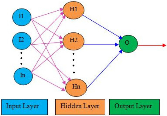
Figure 1.
Multilayer perceptron-based artificial neural network architecture with single layer.
For the purpose of training the multi-layer perceptron neural network, Levenberg–Marquardt, a fast convergence supervised back propagation learning algorithm, was used. Quicker response, robustness, flexibility, ease of programming and simplicity are the main benefits of this algorithm [91]. This algorithm updates the network’s connections and bias weights. It was considered the best choice to supervise the network [92]. The ANN approach which, is trained using the Levenberg–Marquardt algorithm, took the weight update rule, derived from the Newton’s method with steepest descent [93], can be expressed as below:
where “e” represents the error vector, “W” represents the weight vector, “J” represents the Jacobian matrix, identity matrix is represented by “I”, “k” represents iteration number, and “µ” represents the combinational of the Levenberg–Marquardt coefficient. When “µ” is low and approximated to zero value, the Levenberg–Marquardt algorithm behaves like a Newton technique, but when “µ” is high, it behaves like a gradient descent solution with a small size of step [94]. As a result, parameter selection becomes a difficult problem in the Levenberg–Marquardt technique, which was performed iteratively employing optimization inside the algorithm. The error vector values ‘e’ were derived by subtracting the predicted output from the real output. The error was returned to each neuron, which adjusts the bias weights and connection weights across the ANN. By considering the e partial derivatives against all variables that are unknown, such as bias weights and connection weights, the Jacobian matrix was created.
Although ANN has several advantages, such as adaptive training, parallel computing, fault tolerance capability etc. It has a limitation in the processing of vague data. The poor ANN model’s parameters selection causes overfitting and underfitting problems. These limitations of ANN inspired the research to use various approaches of ANN in combination with optimization techniques to address these shortcomings. Nowadays, optimization approaches have become an integral part of modeling in which GA is the one capable global solution approaches. The GA can work as a problem-solving technique in terms of searching, adapting and learning in a variety of applications, particularly for those issues where nonlinear data and complexity of models produce results. In this study, the GA was used for selecting all optimum parameters of the ANN model at a time automatically using hybrid GA-ANN techniques.
2.3. MLR Model
The conventional MLR is a statistical strategy attempt to keep the linear relation among the various inputs (independent) variables by adjusting the linear equation to data and predicting the output i.e., SSY. Mathematically, MLR can be represented by an equation:
where, a represents the regression intercept, b represents the coefficient of input variable water discharge (WD) and c represents the coefficient of water level (WL). The values ‘a’, ‘b’ and ‘c’ were determined by using least square regression method among the input variables and obtained output variables [18,95]. In order to develop the higher order MLR models, there was no need to consider interaction effects of different input variables.
2.4. SRC Model
The SRC, also known as the power relation model, is commonly employed to maintain the nonlinear relationship among the output and input variable. It quantifies the amount of SSY corresponding to the WD measured [43]. The SRC method used in this study established a connection of power between the WD and SSY based on the record of streamflow [96,97]. The power equation of SRC is given below [17,21]:
where, S and Q specify the amount of SSY and WD, respectively. The values of b and a are the rating coefficients attained by using least square regression between log Q and log S.
3. Data Analysis of Study Region
3.1. Study Region
The Godavari River Basin stands as the second longest river in India after Ganga and accounts for 9.5% of the country’s total geographic area. It originates from Central India’s Western Ghat near the hills of Triambakeswar at 1067 m elevation in the Nasik region of Maharashtra, nearly eighty kilometers from the Arabian Sea (Godavari Basin Govt. of India [98]). This basin’s overall drainage area extends up to 312,812 Square kilometer with its greatest length (995 km) and width (583 km). It is one of India’s biggest river basins. It flows east for 1465 km draining Maharashtra, Andhra Pradesh, Telangana, Chhattisgarh Odisha, Madhya Pradesh, Karnataka and Puducherry with 48.6 percent, 23.7 percent, 8.8 percent, 12.4 percent, 5.7 percent, 10 percent, 1.4 percent, 0.01 percent, respectively. The Godavari River Basin lies within a geographical coordinate of 73°24′ to 83°4′ east longitudes and 16°19′ to 22°34′ north latitudes.
Godavari River Basin consists of 16 tributaries which are classified into left bank and right bank that forms an inter-state river system. The major tributaries of the left bank include Pranhita, Sabari, Purna and Indravati which occupies 59.7 percent of the overall drainage area of the Godavari River Basin, and the right bank includes Majira, Pravara and Manair together covering 16.1 percent of the Godavari River Basin. The majority part of the basin is enclosed by agricultural land which occupied 59.57% of the total basin area, followed by forest at 26.16%, water bodies at 2.06% in the form of tanks, reservoirs, ponds, lakes etc. and wasteland at 3.83% as per the evaluation of land Cover and Land use during the period 2005–2006. It falls in the Deccan Plateau with a tropical climate. The climate of the basin in northeastern and western area is colder than the rest from mid-October to mid-February. During south–west monsoons the basin has a maximum rainfall.
Generally, the basin’s predominant types of soils include alkaline, black soil, red soil, mixed, saline, lateritic, and alluvium soils etc. It also contains various wealth minerals such as iron, bauxite, manganese and coal. Other minerals such as lead, zinc, kaolin are available in low quantities in different regions of the basin. In order to enhance the irrigation potential, industrial water supply, hydropower generation and to reduce the regional imbalance, the National Water Development Agency has proposed four inter-basin transfer links that transfer the water from surplus regions to deficit areas. In this study, the data were collected at Polavaram, the last measuring point of the Godavari River Basin, before the sediment loads were discharged into the Bay of Bengal. A map of the location of the Polavaram site is given in Figure 2. Owing to its strategic location and the presence of hydrological factors such as gauge, WD and SSY, it was chosen as a study site for this research.
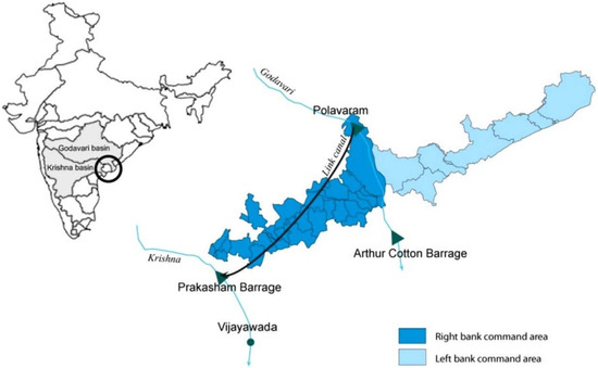
Figure 2.
Location of Polavaram site in Godavari River Basin, Andhra Pradesh, India [98].
3.2. Statistical Data Analysis
The daily mean of WD, WL and SSY data at the Polavaram location of Godavari were taken in this research work. The observation period taken for the daily mean WD, WL and SSY were 45 years during January 1969 to November 1988. Table 1 shows the statistical constraints of the hydrological and climatical data such as minimum (Xmin), standard deviation (SD), mean (Xmean), overall maximum (Xmax) values, skewness, variation coefficient (Cv) and the ratio of maximum to mean. It can be observed that SSY, WL and WD are positively skewed which means relatively asymmetric. Negative skewness explains a distribution which achieves more negative (lesser than average) values, whereas positively skewed explains a distribution which attains more positive (greater than average) values. During this study, the skew value ranges from 1.476 to 4.538, this is supposed to be high because it is greater than 1. SSY has the highest skewness values. A higher skewed value has a more negative impact on the ANN’s performance [99]. It is detected that SSY has the highest coefficient of variation (Cv), standard deviation (SD) and max/mean values among all parameters which show that SSY has a more scattered nature and erratic behavior as compared with WD and WL. These statistical analyses reveal that SSY has maximum variability and complex nonlinear behaviors. From Figure 3, it is noticed that the SSY varies nonlinearity in proportion to WD and WL.

Table 1.
Statistics constraints of hydrological and climatical data at Polavaram, Godavari River Basin.
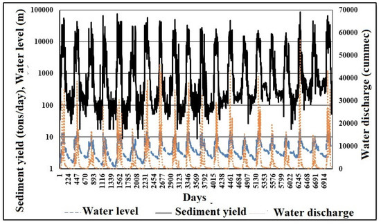
Figure 3.
Variations in daily mean of hydro climatic data: SSY (tons/day), WL (m) and WD (cummec) at the Polavaram in Godavari River Basin.
Pearson correlation coefficient (PCC or denoted by ‘r’) and spearman rank-order correlation (SRC or denoted by Greek letter ‘rho’) are other important statistical measures which were used to understand the relationship between two variables. The PCC determines the linear correlation among two variables, whereas the SRC determines the statistical dependency among the rankings of two variables. The value of PCC varies in the range of minus one and plus one and, where minus one indicates a perfect inverse linear relationship, the 0 value shows that there is no linear relationship. Further, the value plus one denotes a linear correlation that is positive. Table 2 and Table 3 represent the correlation of Pearson (r), and spearman ranks relation between WD and sediment data. It was observed that the values of PCC and SRC are found to be high between two variables, which mean that suspended deposit is highly significantly connected to the WD and WL.
Table 2.
Pearson Correlation coefficient of data at Polavaram, Godavari River Basin.
Table 3.
Spearman’s rank correlation coefficient of data at Polavaram, Godavari River Basin.
The analysis of variance testing is used to check that the SSY, WL and WD data set are significantly different or not. This can be done by comparing the means of different data samples from the datasets. The analysis of variance null hypothesis is rejected, indicating that there is no similarity relationship among these SSY, WD and WL variables. The box graph of SSY, WL and WD datasets is displayed in Figure 4, indicating that they are all distinct due to variances in the box center lines. It was therefore decided that WD and WL are important inputs features to predict SSY.
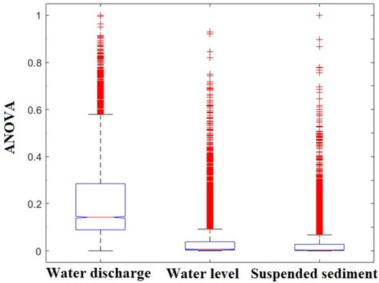
Figure 4.
Analysis of variance test result of WD, WL and SSY.
3.3. Data Preparation and Data Processing
Before training the ANNs, data normalization was a very important step. The main aim of data normalization is to eliminate data redundancies, difference in dimensionality and maintain equity between variables [100,101,102]. During training, it improves the speed of processing and convergence which in turn helps in reducing the errors in prediction. Therefore, normalization was done prior to training with the model after collecting the hydro climatic data. The normalization of data between 0 and 1 can be carried out using Equation (6). Instead of original data, normalized data can be used in all the models such as MLR, SRC, GA-ANN and ANN.
where, Dnorm represents the normalized value, Di indicates ith original value, Dmax and Dmin represents the max and min values of the data.
After normalization, the dataset was divided into different sets such as validation, testing and training for the development of robust and accurate models. Training requires 70% of data used for training purpose in the neural network-based models, while the remaining 30% data were shared equally through the processes of validation and testing to eliminate the over- and under fitting issues in the network [56,103]. Nineteen and a half years of daily hydro-metrological data (1969–1988) of WD, WL and SSY were utilized for proposed modeling. In this study, data used for training were taken between 1 June 1969 and 24 January 1983, for validation between 25 January 1983 and 27 December 1985 and for testing between 28 December 1985 and 30 November 1988. Data were not continuously selected for validation and training to prevent the model from overfitting problems [103].
4. Results and Discussion
4.1. GA-ANN
Matlab software with customized code was applied to develop the hybrid GA-ANN model. The features in the ANN model were selected on the basis of the normalized data. In this study, the number of generations (n) was taken as the criterion for stopping and contains the highest value 50. The proposed hybrid GA-ANN model was provided final optimum solutions set at stopping criterion. Figure 5 depicts the fluctuations in the mean fitness value and RMSE values of each generation in the GA-ANN model throughout the training stage. The minimum value of RMSE was equal to 0.0322602 which is the best fitness amongst all generations and its corresponding mean fitness value was equal to 0.0322602. It is also seen that the value of the mean fitness function of each generation of the GA remained unaltered after generation count 8 (Figure 5). The hidden layer neurons that worked best was 31. It should be noted that the highest fitness value of each generation remains unchanged after 10 generations. The continuous and monotonically increasing activation function, namely tan-sigmoidal, was optimally chosen for the output layer and hidden layer. The GA-ANN chose the optimum µ as 43 in the Levenberg–Marquardt algorithm. After maximum generation, the chromosome corresponding to best fitness is taken as an optimum parameter in the GA-ANN model.
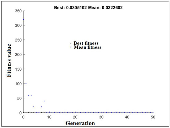
Figure 5.
Generation-wise RMSE profile of GA-ANN model.
To assess the effectiveness of the models, statistical metrics such as correlation coefficient (r), mean square error (MSE), coefficient of determination (R2), mean absolute error (MAE), error variance (VAR) and root mean square error (RMSE) were utilized.
where, , , and are measured, measured mean, predicted, and predicted mean values respectively. The N value represents the number of samples. The E and represent the error and mean error values.
Table 4 summarizes the statistics of error of the generated GA-ANN model’s testing, validation and training datasets. According to this table, the MAE and RMSE values of the data sets are quite low, but the R2 value is very high. According to the statistical findings, it is demonstrated that the constructed GA-ANN model achieved a higher accuracy in predicting the SSY. Because of the low error parameters and strong R2 values, the model was protected from over and underfitting. The best hybrid GA-ANN model was constructed to predict SSY utilizing with just WD and WL as input parameters. The error statistics data also reveal that MAE and RMSE had comparable types of patterns. The results reveal a direct proportional association between RMSE, variance, and MAE statistics data. These results also reveal that MAE, variance and RMSE had comparable types of patterns.
Table 4.
Error statistics of GA-ANN model at Polavaram, Godavari River Basin.
In addition to quantitative assessment making use of statistical indicators, the effectiveness of the GA-ANN method in estimating the SSY was evaluated by diagrammatic illustrations. The hydrograph and scatter diagrams of estimated and observed SSY are shown in the Figure 6. It was also noticed from the scatter and hydrograph plots that high, low and medium magnitudes of SSY prediction values by the GA-ANN model are close to actual values of SSY. It was also noticed that the positive SSY values are calculated by the proposed GA-ANN model corresponding to approximated to zero or low values of actual SSY (Figure 6a,b). This result shows that ANN in conjunction with GA has the maximum accurate method for finding the SSY in Godavari River Basin system. It can be seen in past research that in many river basin systems, some artificial intelligence-based techniques have predicted negative SSY values [3,19,87,104]. It is revealed that SSY has complex non-linear and erratic behavior at the low-level values of sediment yield. It is very difficult to handle these complex sedimentation phenomena. However, this is entirely impracticable. SSY always shows positive values in nature. In contrast, the proposed GA-ANN models predicted all positive SSY values corresponding to high, medium as well as low observed sediment values. Thus, it demonstrates the fact that the GA-based ANN technique has more generalization capability and provided satisfactory performance.
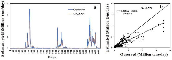
Figure 6.
(a) Hydrograph and (b) scatter plot based on test data between the predicted GA-ANN SSY and observed SSY.
The calculated SSY values using the GA-ANN approaches are very near to the actual sediment yield values shown in Figure 6a. It is seen from the scatter diagram and hydrograph that the degree of high, moderate, and low SSY prediction values by the ANN approach are nearer to the actual SSY values. The scatter plot of Figure 6b illustrates that a greater number of points lie very nearer to the bisector line which inferred that the original and model predicted values are significantly almost same.
4.2. ANN
The ANN model was made using output, inputs, and a single layer of hidden neurons. For the selection of hidden neurons and learning parameters in the ANN model, methods of trial and error were utilized. During the ANN model training, the value of learning parameter (µ) varied from 0.001 to a maximum 10 × 109; and the value of µ decreased and increased by a factor of 0.10 and 10, respectively. The proposed GA-ANN model started with an initialized µ value and changed the value for each epoch to enhance the ANN’s accuracy. The optimum value of neurons and µ value in the single hidden layer of the ANN technique is equal to 30 and 0.001, respectively.
Table 5 represents the performance evaluations of the ANN technique through the statistical measures such as MAE, RMSE, R2, VAR and MSE in the validation, testing and training states. Table 5 demonstrates that the RMSE (0.0376–0.0538) and MAE (0.0207–0.237) of the ANN technique is very low and r (0.799–0.924) is very high during testing, validation, and training period. These results confirm that SSY prediction by ANN model has much more accurate performance. The lower values of RMSE, MAE, MSE, error variance and higher values of r in testing, validation and training are all nearly close to each other which shows that under-fitted or over-fitted problems were not encountered in the ANN model. After result analysis, it was also found that MAE and RMSE have similar trends. It was also observed that the RMSE varied proportionally to MAE in the ANN model.
Table 5.
Error statistics of ANN model at Polavaram, Godavari River Basin.
It was observed from the graphical representation of the ANN that predicted SSY and observed SSY are similar (Figure 7a). The estimated SSY of the ANN and observed SSY values are very close to the bisector line (forty-five-degree line) in a scatter plot of the ANN model (Figure 7b). The value of the slope in regression line of the ANN model is less than one which reveals that underestimation, this is also supported by the hydrograph (Figure 7a). It is also noticed that negative SSY values were calculated by the ANN model at low or approximated to zero SSY. This demonstrates that the ANN method is not able to record the complex SSY behavior at low observed values. SSY cannot be negative in reality. This reveals that the small valued SSY data have a highly erratic and non-linear nature.
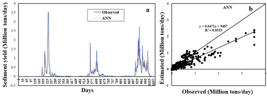
Figure 7.
(a) Hydrograph and (b) scatter plot based on test data between the ANN predicted SSY and observed SSY.
4.3. MLR
The MLR model predicts SSY using the WD and WL data as input variables. Table 6 shows the statistical errors determined by the MLR method. The MLR model is trained and developed on the basis of training data. The validation data set is not used in the MLR model because it has no overfitting issues. The MLR model uses the same testing data as the GA-ANN, SRC, and ANN models. The values of the MLR model’s a, b, and c coefficients are 0.0076, 0.00745 and 0.6181, respectively. Table 6 shows the statistical error analysis of the MLR model, which is generated using the MLR predicted SSY and observed SSY for the training and testing datasets. It was observed that there are low values of RMSE (0.038723–0.054473) and MAE (0.017119–0.020384) and high values of r (0.791669–0.92169). The lower value of MAE and RMSE and higher value of r in testing phase demonstrates that the MLR method judiciously fit the data set. The training data set also shows these types of behaviors. It is obvious that the linear MLR model has no overfitting problem during the training phase. The values of MAE and RMSE in the MLR model during the testing are 0.020384 and 0.054473, respectively. The RMSE and MAE are varied directly proportional to each other during validation and training period which is also obvious of the linear model. The significant error variance of the data set during the testing phase demonstrates that the MLR model is unable to capture data variability, which might be related to the existence of complex non-linearity.
Table 6.
Error statistics of MLR model at Polavaram, Godavari River Basin.
It could be noted that this model gives a negative value at lower sediment rates which is not real estimation (Figure 8). The comparison plot of predicted SSY and observed SSY is depicted in Figure 8a. Figure 8b illustrates that some data points lie along the line of the bisector where observed and estimated values are identical. On the other hand, the SSY is estimated negative values by MLR model at lower SSY values which means that for smaller sample values, data exhibit a strong non-linear behavior. Therefore, the non-linearity of SSY data are not captured by this linear MLR model which therefore predicts a negative SSY value.
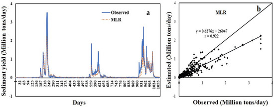
Figure 8.
(a) Hydrograph and (b) scatter plot based on test data between the MLR predicted SSY and observed SSY.
4.4. SRC
The SRC curve coefficient was calculated by using a least square regression method in log scale which is then converted in original scale by back transfer approaches. The calculated value coefficients b and a in SRC method are given as 1.0799 and 0.4379, respectively. Table 7 lists the error statistics of the SRC method. It can be seen from Table 7 that the SRC method has the lowest r value (0.9004) and greatest RMSE (0.061759) during training period whereas it has highest RMSE (0.082824) and higher r (0.917363) during testing period. The SRC model has lowest RMSE (0.031131) and highest r (0.99081) during validation period. This indicates that here is no similar type of pattern between the RMSE and r during training, validation and testing phase.
Table 7.
Error statistics of SRC model at Polavaram, Godavari River Basin.
The hydrograph and scatter graph of the SRC model among the observed and expected sediment production are displayed in Figure 9. According to the scatter plot and hydrograph between predicted and actual suspended sediment production, this SRC approach yields an underestimated value for extremely high sediment yield (Figure 9a,b). The SRC method’s negative mean error (−0.0310) value likewise reveals the underestimating of sediment output. The value of slope of the linear regression is smaller than the slope of the 45-degree line which is shown in the scatter diagram Figure 9b. The scatter plot also shows that scatter points mainly fall around the 45-degree line, except for high sediment yield values, which are greatly overestimated and fall considerably below. A similar underestimating of the expected suspended production has been seen in various rivers of the United States [18,19,105,106,107,108]. This discrepancy is mostly due to the particular use of WD as an input variable, rather than other characteristics that play an indirect or direct impact in sediment yield creation in river basins.
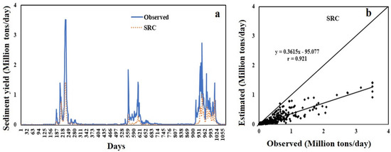
Figure 9.
(a) Hydrograph and (b) scatter plot based on test data between the SRC predicted and observed SSY.
4.5. Comparative Assessment of Various Models on the Basis of Testing Data Set
The performance of the developed GA-ANN model was verified using the test dataset, which consists of unseen data that were not utilized in the model development during the training period. The RMSE, MAE, and R2 statistical metrics were employed during testing for all ANN, GA-ANN, SRC and MLR models with optimized parameters of the models demonstrated in Table 8. Performances of the GA-ANN model were compared with SRC, MLR and ANN models. During the testing phase, all of the models utilized the identical SSY dataset. The comparison was based on estimated SSY and observed SSY of testing data. It can be observed that the proposed hybrid novel GA-ANN technique provided better results on the basis of R2 and RMSE as compared with the conventional models.
Table 8.
Performance comparison of various models with optimum parameters. Bold values show the best results.
The SSY in the hydrographs of ANN and GA-ANN models are approximately closer to actual data as compared with conventional SRC and MLR models. The conventional SRC model provided very poor performance, which produced high underestimation at the peaks. Therefore, this model was incapable of recording high SSY. The scatter plot and hydrograph demonstrate that the MLR and ANN models predicted the negative sediments at lower sediment values similar to the previous study [3,18,19,87,104] but it is absolutely impractical because the SSY may not contain the negative values. The proposed GA-ANN technique gave the positive values of SSY for moderate, high and low SSY. By considering all these findings, it is found that the GA-ANN hybrid model has achieved best performance and higher generalization ability as compared to other models. Moreover, it is noted from the hydrographs that predicted SSY by the GA-ANN model is more closely related to the observed data as compared with ANN, SRC and MLR methods, specifically at large values of SSY (Figure 6a, Figure 7a, Figure 8a and Figure 9a). The SRC method presented poor performances which caused significant underestimation at the peaks. This result demonstrates that this method is capable of recording usually high SSY. In the scattered graph, it can be seen that the MLR and ANN models predicted negative values of SSY at low value (Figure 7b and Figure 8b). This is an entirely impractical prediction of SSY which, in nature, exit as positive values. The GA-ANN predicted a positive SSY even when the observed SSY is lower. It provides a positive SSY for moderate, high and low SSY. Thus, GA-ANN looks to have the most potential and generalized robust model in comparison to another models. The results demonstrate that the GA-ANN technique has shown a reasonable satisfactory performance and has a greater capacity to generalize. This advantage of the proposed GA-ANN works because all parameters of the ANN model are optimized at the same time using the GA. It is also reported that both artificial intelligence-based models such as GA-ANN and ANN outperform the classic SRC and MLR regression methods.
5. Conclusions
This study described the prediction of SSY using SRC, MLR, ANN and GA-ANN models in the Godavari River Basin at Polavaram, Andhra Pradesh, India, by taking WD and WL data as inputs. It is observed that WL and WD are the most important parameters for estimating SSY. An effective ANN structure is created in conjunction with GA to calculate SSY in order to improve the ANN structure. In comparison with ANN, SRC and MLR, the GA-ANN model predicts extremely high, medium, and low suspended sediments values with more accuracy and generalization. As a result, it is hypothesized that the proposed GA-ANN model may be a desirable substitute for classical methods such as SRC, ANN and MLR. Using WD and WL as input parameters. The GA-ANN model provided a relatively accurate SSY estimate. Summarizing, the magnitudes of small, high and medium SSY given by the GA-ANN technique were very close to observed values as compared with other classical methods. This superiority was achieved when all ANN parameters were optimized simultaneously using GA. This research demonstrates that parameter choice not only increases model efficiency but also decrease the computational period considerably by avoiding trial-and-error methods and grid search approaches.
The main aim of this study was the concurrent optimization of various ANN parameters to predict SSY accurately. These findings have realistic importance such that few inputs (WD and WL) can be used to assess the daily SSY of Godavari River Basin by training the ANN with GA. This strategy will be helpful in improving the management of water resources for the downstream region as well as in designing pipes, canals, bridges, dams and watershed management issues in the Godavari River Basin, India. This research used the information from Polavaram station only and further research may be needed to strengthen these findings by using more information taken from different gauge stations. In future, various kinds of ANN models in conjunction with GA will be tested by using more controlling factors of sediment like R, T, runoff and spatial data.
Author Contributions
Conceptualization, A.Y.; methodology, A.Y.; software, A.Y.; C.I., T.R.G., validation, A.Y.; V.K. and D.J.; formal analysis, C.I., T.R.G., A.Y.; investigation, A.Y.; resources, A.Y.; writing—review and editing, C.I., T.R.G., A.Y., V.K., D.J. and H.M.; writing—original draft preparation, A.Y.; supervision, C.I., T.R.G., A.Y. The paper has been read and approved by all authors. All authors have read and agreed to the published version of the manuscript.
Funding
This research received no external funding.
Institutional Review Board Statement
Not Applicable.
Informed Consent Statement
Not Applicable.
Data Availability Statement
The data used in the study were obtained after signing a non-disclosure agreement with the Central Water Commission (CWC). As a result, they cannot be shared. However, the solutions can be shared. Please contact the first author with proper justification.
Acknowledgments
The authors thank the Government (India-WRIS) of India for providing free data and support. The author appreciates the Koneru Lakshmaiah Educational Foundation, India, for offering the necessary facilities for this research.
Conflicts of Interest
The authors declare no conflict of interest.
References
- Sivakumar, B. Suspended sediment load estimation and the problem of inadequate data sampling: A fractal view. Earth Surf. Processes Landf. 2005, 31, 414–427. [Google Scholar] [CrossRef]
- Taniguchi, T. Observation of sediment load in the river with the thiltmeter (with the tiltmeter of zöllner suspension). Hydrol. Sci. J. 1958, 3, 22–32. [Google Scholar] [CrossRef][Green Version]
- Cigizoglu, H.K. Estimation and forecasting of daily suspended sediment data by multi-layer perceptrons. Adv. Water Resour. 2004, 27, 185–195. [Google Scholar] [CrossRef]
- Cobaner, M.; Unal, B.; Kisi, O. Suspended sediment concentration estimation by an adaptive neuro-fuzzy and neural network approaches using hydro-meteorological data. J. Hydrol. 2009, 367, 52–61. [Google Scholar] [CrossRef]
- Mukherjee, S.; Veer, V.; Tyagi, S.K.; Sharma, V. Sedimentation study of Hirakud reservoir through remote sensing techniques. J. Spat. Hydrol. 2007, 7, 122–130. [Google Scholar]
- Hsieh, T.-C.; Ding, Y.; Yeh, K.-C.; Jhong, R.-K. Numerical Investigation of Sediment Flushing and Morphological Changes in Tamsui River Estuary through Monsoons and Typhoons. Water 2022, 14, 1802. [Google Scholar] [CrossRef]
- Lee, F.Z.; Lai, J.S.; Sumi, T. Reservoir Sediment Management and Downstream River Impacts for Sustainable Water Resources—Case Study of Shihmen Reservoir. Water 2022, 14, 479. [Google Scholar] [CrossRef]
- Hsieh, T.C.; Ding, Y.; Yeh, K.C.; Jhong, R.K. Investigation of morphological changes in the tamsui river estuary using an integrated coastal and estuarine processes model. Water 2020, 12, 1084. [Google Scholar] [CrossRef]
- Pektas, A.O.; Cigizoglu, H.K. Long-range forecasting of suspended sediment. Hydrol. Sci. J. 2017, 62, 2415–2425. [Google Scholar] [CrossRef]
- FEMA [Federal Emergency Management Agency]. National Dam Safety Program. 1999. Available online: http://www.fema.gov/mit/ndspweb.htm (accessed on 10 April 2022).
- Evans, J.E.; Mackey, S.D.; Gottgens, J.F.; Gill, W.M. Lessons from a dam failure. Ohio J. Sci. 2000, 100, 121–131. [Google Scholar]
- Duan, W.L.; He, B.; Takara, K.; Luo, P.; Nover, D.; Hu, M.C. Modeling suspended sediment sources and transport in the Ishikari River basin, Japan, using SPARROW. Hydrol. Earth Syst. Sci. 2015, 19, 1293–1306. [Google Scholar] [CrossRef]
- Gaurav, K.; Sinha, R.; Panda, P.K. The Indus flood of 2010 in Pakistan: A perspective analysis using remote sensing data. Nat. Hazards 2011, 59, 1815–1826. [Google Scholar] [CrossRef]
- ZICL. Risk Nexus. In Urgent Case for Recovery: What We Can Learn from the August 2014 Karnali River Foods in Nepal; Zurich Insurance Group Ltd.: Zurich, Switzerland, 2014. [Google Scholar]
- Kisi, O.; Shree, J. River suspended sediment estimation by climatic variables implication: Comparative study among soft computing techniques. Comput. Geosci. 2012, 43, 73–82. [Google Scholar] [CrossRef]
- Melesse, A.M.; Ahmad, S.; McClain, M.E.; Wang, X.; Lim, Y.H. Suspended sediment load prediction of river systems: An artificial neural network approach. Agric. Water Manag. 2011, 98, 855–866. [Google Scholar] [CrossRef]
- Zhu, Y.M.; Lu, X.X.; Zhou, Y. Suspended sediment flux modeling with artificial neural network: An example of the Longchuanjiang River in the Upper Yangtze Catchment, China. Geomorphology 2007, 84, 111–125. [Google Scholar] [CrossRef]
- Yadav, A.; Chatterjee, S.; Equeenuddin, S.M. Prediction of suspended sediment yield by artificial neural network and traditional mathematical model in Mahanadi River basin, India. Sustain. Water Resour. Manag. 2018, 4, 745–759. [Google Scholar] [CrossRef]
- Yadav, A.; Chatterjee, S.; Equeenuddin, S.M. Suspended sediment yield estimation using genetic algorithm-based artificial intelligence models: Case study of Mahanadi River, India. Hydrol. Sci. J. 2018, 63, 1162–1182. [Google Scholar] [CrossRef]
- Oltman, D.O. Statistics for Business and Economics; McGraw-Hill Publishing: New York, NY, USA, 1990; p. 1117. [Google Scholar]
- Jain, S.K. Development of integrated sediment rating curves using ANNs. J. Hydraul. Eng. 2001, 127, 30–37. [Google Scholar] [CrossRef]
- McBean, E.A.; Al-Nassri, S. Uncertainty in suspended sediment transport curves. J. Hydraul. Eng. 1988, 114, 63–74. [Google Scholar] [CrossRef]
- Lenzi, M.A.; Marchi, L. Suspended sediment load during floods in a small stream of the Dolomites (northeastern Italy). Catena 2000, 39, 267–282. [Google Scholar] [CrossRef]
- Khoi, D.N.; Suetsugi, T. The responses of hydrological processes and sediment yield to land-use and climate change in the Be River Catchment, Vietnam. Hydrol. Process 2014, 28, 640–652. [Google Scholar] [CrossRef]
- Buendia, C.; Bussi, G.; Tuset, J.; Vericat, D.; Sabater, S.; Palau, A.; Batalla, R.J. Effects of afforestation on runoff and sediment load in an upland Mediterranean catchment. Sci. Total Environ. 2016, 540, 144–157. [Google Scholar] [CrossRef] [PubMed]
- Kingston, G.B.; Dandy, G.C.; Maier, H.R. Review of artificial intelligence techniques and their applications to hydrological modeling and water resources management Part 2–optimization. Water Resour. Res. 2008, 61, 67–99. [Google Scholar]
- Razia, S.; Narasingarao, M.R.; Bojja, P. Development and analysis of support vector machine techniques for early prediction of breast cancer and thyroid. J. Adv. Res. Dyn. Control Syst. 2017, 9, 869–878. [Google Scholar]
- Chakravorti, T.; Satyanarayana, P. Nonlinear system identification using kernel based exponentially extended random vector functional link network. Appl. Soft Comput. 2020, 89, 106–117. [Google Scholar] [CrossRef]
- Anila, M.; Pradeepini, G. Study of prediction algorithms for selecting appropriate classifier in machine learning. J. Adv. Res. Dyn. Control Syst. 2017, 9, 257–268. [Google Scholar]
- Hussain, M.A.; Jayanthi, A. Novel Approach Certificate Revocation in MANET using Fuzzy Logic. Indones. J. Electr. Eng. Comput. Sci. 2018, 10, 654–663. [Google Scholar] [CrossRef]
- Patel, A.K.; Chatterjee, S.; Gorai, A.K. Development of an expert system for iron ore classification. Arab. J. Geosci. 2018, 11, 401. [Google Scholar] [CrossRef]
- Ramaiah, P.; Kumar, S. Dynamic analysis of soil structure interaction (SSI) using ANFIS model with oba machine learning approach. Int. J. Civ. Eng. Technol. 2018, 9, 496–512. [Google Scholar]
- Patel, A.K.; Chatterjee, S.; Gorai, A.K. Development of a machine vision system using the support vector machine regression (SVR) algorithm for the online prediction of iron ore grades. Earth Sci. Inform. 2019, 12, 197–210. [Google Scholar] [CrossRef]
- Patel, A.K.; Chatterjee, S.; Gorai, A.K. Effect on the performance of a support vector machine-based machine vision system with dry and wet ore sample images in classification and grade prediction. Pattern Recognit. Image Anal. 2019, 29, 309–324. [Google Scholar] [CrossRef]
- Dabbakuti, J.R.K.K.; Bhavya, L.G. Application of singular spectrum analysis using artificial neural networks in TEC predictions for ionospheric space weather. IEEE J. Sel. Top. Appl. Earth Obs. Remote Sens. 2019, 12, 5101–5107. [Google Scholar] [CrossRef]
- Dabbakuti, J.R.K.K.; Jacob, A.; Veeravalli, V.R.; Kallakunta, R.K. Implementation of IoT analytics ionospheric forecasting system based on machine learning and ThingSpeak. IET Radar Sonar Navig. 2019, 14, 341–347. [Google Scholar] [CrossRef]
- Ranjeeta, B.; Chakravorti, T.; Nayak, N.R. A hybrid Hilbert Huang transform and improved fuzzy decision tree classifier for assessment of power quality disturbances in a grid connected distributed generation system. Int. J. Power Energy Convers. 2020, 11, 60–81. [Google Scholar]
- Bhattacharya, B.; Lobbrecht, A.H.; Solomatine, D.P. Neural networks and reinforcement learning in control of water systems. J. Water Resour. Plan Manag. 2003, 129, 458–465. [Google Scholar] [CrossRef]
- Wang, Y.M.; Traore, S. Time-lagged recurrent network for forecasting episodic event suspended sediment load in typhoon prone area. Int. J. Phys. Sci. 2009, 4, 519–528. [Google Scholar]
- Singh, G.; Panda, R. Daily sediment yield modeling with artificial neural network using 10-fold cross validation method: A small agricultural watershed, Kapgari, India. Int. J. Earth Sci. Eng. 2011, 6, 43–450. [Google Scholar]
- Tayfur, G. Artificial neural networks for sheet sediment transport. Hydrol. Sci. J. 2002, 47, 879–892. [Google Scholar] [CrossRef]
- Kisi, Ö. Multi-layer perceptrons with Levenberg-Marquardt training algorithm for suspended sediment concentration prediction and estimation/Prévision et estimation de la concentration en matières en suspension avec des perceptrons multi-couches et l’algorithme d’apprentissage de Levenberg-Marquardt. Hydrol. Sci. J. 2004, 49, 1025–1040. [Google Scholar]
- Kisi, O. Suspended sediment estimation using neuro-fuzzy and neural network approaches. Hydrol. Sci. J. 2005, 50, 683–696. [Google Scholar] [CrossRef]
- Jothiprakash, V.; Garg, V. Reservoir sedimentation estimation using artificial neural network. J. Hydrol. Eng. 2009, 14, 1035–1040. [Google Scholar] [CrossRef]
- Patil, R.A.; Shetkar, R.V. Prediction of sediment deposition in reservoir using artificial neural networks. Int. J. Civ. Eng. Technol. 2016, 7, 1–12. [Google Scholar]
- Toriman, E.; Jaafar, O.; Maru, R.; Arfan, A.; Ahmar, A.S. Daily Suspended Sediment Discharge Prediction Using Multiple Linear Regression and Artificial Neural Network. J. Phys. Conf. Ser. 2018, 954, 012030. [Google Scholar]
- Kisi, O. Constructing neural network sediment estimation models using a data-driven algorithm. Math. Comput. Simul. 2008, 79, 94–103. [Google Scholar] [CrossRef]
- Bishop, M.C. Neural Networks for Pattern Recognition; Oxford Clarendon Press: Oxford, UK, 1998. [Google Scholar]
- Yadav, A.; Chatterjee, S.; Equeenuddin, S.M. Suspended sediment yield modeling in Mahanadi River, India by multi-objective optimization hybridizing artificial intelligence algorithms. Int. J. Sediment. Res. 2021, 36, 76–91. [Google Scholar] [CrossRef]
- Yadav, A.; Satyannarayana, P. Multi-objective genetic algorithm optimization of artificial neural network for estimating suspended sediment yield in Mahanadi River basin, India. Int. J. River Basin Manag. 2020, 18, 207–215. [Google Scholar] [CrossRef]
- Yadav, A. Estimation and Forecasting of Suspended Sediment Yield in Mahanadi River Basin: Application of Artificial Intelligence Algorithms; NIT Rourkela: Orissa, India, 2020. [Google Scholar]
- Yadav, A.; Prasad, B.B.V.S.V.; Mojjada, R.K.; Kothamasu, K.K.; Joshi, D. Application of Artificial Neural Network and Genetic Algorithm Based Artificial Neural Network Models for River Flow Prediction. Rev. Intell. Artif. 2020, 34, 745–751. [Google Scholar] [CrossRef]
- Zhang, D.; Xiao, J.; Zhou, N.; Zheng, M.; Luo, X.; Jiang, H.; Chen, K. A genetic algorithm based support vector machine model for blood-brain barrier penetration prediction. BioMed Res. Int. 2015, 2015, 292683. [Google Scholar] [CrossRef]
- Chatterjee, S.; Bandopadhyay, S. Goodnews bay platinum resource estimation using least square support vector regression with selection of input space dimension and hyperparameters. Nat. Resour. Res. 2011, 20, 117–129. [Google Scholar] [CrossRef]
- Su, J.; Wang, X.; Liang, Y.; Chen, B. GA-based support vector machine model for the prediction of monthly reservoir storage. J. Hydrol. Eng. 2014, 19, 1430–1437. [Google Scholar] [CrossRef]
- Adib, A.; Mahmoodi, A. Prediction of suspended sediment load using ANN GA conjunction model with markov chain approach at flood conditions. KSCE J. Civ. Eng. 2017, 21, 447–457. [Google Scholar] [CrossRef]
- Altunkaynak, A. Adaptive estimation of wave parameters by Geno-Kalman filtering. Ocean Eng. 2008, 35, 1245–1251. [Google Scholar] [CrossRef]
- Topchy, A.P.; Lebedko, O.A.; Miagkikh, V.V. Fast learning in multilayered neural networks by means of hybrid evolutionary and gradient algorithms. In Proceedings of the IC on Evolutionary Computation and Its Applications, Moscow, Russia, June 1996. [Google Scholar]
- Nasseri, M.; Asghari, K.; Abedini, M.J. Optimized scenario for rainfall forecasting using genetic algorithm coupled with artificial neural network. Expert Syst. Appl. 2008, 35, 1415–1421. [Google Scholar] [CrossRef]
- Gowda, C.C.; Mayya, S.G. Comparison of back propagation neural network and genetic algorithm neural network for stream flow prediction. J. Comput. Environ. Sci. 2014, 2014, 290127. [Google Scholar] [CrossRef]
- Ding, Y.R.; Cai, Y.J.; Sun, P.D.; Chen, B. The use of combined neural networks and genetic algorithms for prediction of river water quality. J. Appl. Res. Technol. 2014, 12, 493–499. [Google Scholar] [CrossRef]
- Adib, A.; Jahanbakhshan, H. Stochastic approach to determination of suspended sediment concentration in tidal rivers by artificial neural network and genetic algorithm. Can. J. Civ. Eng. 2013, 40, 299–312. [Google Scholar] [CrossRef]
- Malik, A.; Kumar, A.; Piri, J. Daily suspended sediment concentration simulation using hydrological data of Pranhita River Basin, India. Comput. Electron. Agric. 2017, 138, 20–28. [Google Scholar] [CrossRef]
- Paz, E. A Survey of Parallel Genetic Algorithms. 1998. Available online: http://www.www.illigal.ge.uiuc.edu (accessed on 10 April 2022).
- Agrawal, S.; Sarkar, S.; Srivastava, G.; Maddikunta, P.K.R.; Gadekallu, T.R. Genetically optimized prediction of remaining useful life. Sustain. Comput. Inform. Syst. 2021, 31, 100565. [Google Scholar] [CrossRef]
- Agrawal, S.; Sarkar, S.; Alazab, M.; Maddikunta, P.K.R.; Gadekallu, T.R.; Pham, Q.V. Genetic CFL: Hyperparameter Optimization in Clustered Federated Learning. Comput. Intell. Neurosci. 2021, 2021, 7156420. [Google Scholar] [CrossRef]
- Reddy, G.T.; Reddy, M.; Lakshmanna, K.; Rajput, D.S.; Kaluri, R.; Srivastava, G. Hybrid genetic algorithm and a fuzzy logic classifier for heart disease diagnosis. Evol. Intell. 2020, 13, 185–196. [Google Scholar] [CrossRef]
- Goldberg, D.E.; Deb, K. A comparative analysis of selection schemes used in genetic algorithms. In Foundations of Genetic Algorithms; Rawlins, G.J., Ed.; Morgan Kaufmann: San Mateo, CA, USA, 1991; pp. 69–93. [Google Scholar]
- Beyer, H.G. Evolutionary algorithms in noisy environments: Theoretical issues and guidelines for practice. Comput. Methods Appl. Mech. Eng. 2000, 186, 239–267. [Google Scholar] [CrossRef]
- Wang, Q.J. The genetic algorithm and its application to calibrating conceptual rainfall-runoff models. Water Resour. Res. 1991, 27, 2467–2471. [Google Scholar] [CrossRef]
- Liong, S.Y.; Chan, W.T.; ShreeRam, J. Peak-flow forecasting with genetic algorithm and SWMM. J. Hydraul. Eng. 1995, 121, 613–617. [Google Scholar] [CrossRef]
- Cieniawski, S.E.; Eheart, J.W.; Ranjithan, S. Using genetic algorithms to solve a multiobjective groundwater monitoring problem. Water Resour. Res. 1995, 31, 399–409. [Google Scholar] [CrossRef]
- Jain, A.; Srinivasulu, S. Development of effective and efficient rainfall-runoff models using integration of deterministic, real-coded genetic algorithms, and artificial neural network techniques. Water Resour. Res. 2004, 40, 1–12. [Google Scholar] [CrossRef]
- Tayfur, G.; Moramarco, T. Predicting hourly-based flow discharge hydrographs from level data using genetic algorithms. J. Hydrol. 2008, 352, 77–93. [Google Scholar] [CrossRef]
- Altunkaynak, A. Sediment load prediction by genetic algorithms. Adv. Eng. Softw. 2009, 40, 928–934. [Google Scholar] [CrossRef]
- Sirdari, Z.Z.; Ghani, A.A.; Sirdari, N.Z. Bedload transport predictions based on field measurement data by combination of artificial neural network and genetic programming. Pollution 2015, 1, 85–94. [Google Scholar]
- Chatterjee, S.; Bandopadhyay, S. Reliability estimation using a genetic algorithm-based artificial neural network: An application to a laud-haul-dump machine. Expert Syst. Appl. 2012, 39, 10943–10951. [Google Scholar] [CrossRef]
- Davis, L. Handbook of Genetic Algorithms; Van Nostrand Reinhold: Graham, NC, USA, 1991. [Google Scholar]
- Dejong, K. An Analysis of the Behavior of a Class of Genetic Adaptive Systems. Ph.D. Thesis, Department of Computer and Communication Sciences, University of Michigan, Ann Arbor, MI, USA, 1975. [Google Scholar]
- Haghizade, A.; Shui, L.T.; Goudarzi, E. Estimation of yield sediment using artificial neural network at basin scale. Aust. J. Basic Appl. Sci. 2010, 4, 1668–1675. [Google Scholar]
- Reddy, G.T.; Khare, N. Hybrid firefly-bat optimized fuzzy artificial neural network based classifier for diabetes diagnosis. Int. J. Intell. Eng. Syst. 2017, 10, 18–27. [Google Scholar] [CrossRef]
- Panwar, S.; Khan, M.Y.A.; Chakrapani, G.J. Grain size characteristics and provenance determination of sediment and dissolved load of Alaknanda River, Garhwal Himalaya, India. Environ. Earth Sci. 2016, 75, 91. [Google Scholar] [CrossRef]
- Alp, M.; Cigizoglu, H.K. Suspended sediment estimation by feed forward back propagation method using hydro meteorological data. Environ. Model. Softw. 2007, 22, 2–13. [Google Scholar] [CrossRef]
- Kişi, Ö. Streamflow forecasting using different artificial neural network algorithms. J. Hydrol. Eng. 2007, 12, 532–539. [Google Scholar] [CrossRef]
- Fotovatikhah, F.; Herrera, M.; Shamshirband, S.; Chau, K.W.; Faizollahzadeh Ardabili, S.; Piran, M.J. Survey of computational intelligence as basis to big flood management: Challenges, research directions and future work. Eng. Appl. Comput. Fluid Mech. 2018, 12, 411–437. [Google Scholar] [CrossRef]
- Panagoulia, D. Artificial neural networks and high and low flows in various climate regimes. Hydrol. Sci. J. 2006, 51, 563–587. [Google Scholar] [CrossRef]
- Cigizoglu, H.K.; Kisi, O. Methods to improve the neural network performance in suspended sediment estimation. J. Hydrol. 2006, 317, 221–238. [Google Scholar] [CrossRef]
- Bouzeria, H.; Ghenim, A.N.; Khanchoul, K. Using artificial neural network (ANN) for prediction of sediment loads, application to the Mellah catchment northeast Algeria. J. Water Land Dev. 2017, 33, 47–55. [Google Scholar] [CrossRef]
- Hornik, K.; Stinchcombe, M.; White, H. Multilayer feedforward networks are universal approximators. Neural Netw. 1989, 2, 359–366. [Google Scholar] [CrossRef]
- Tang, Z.; De Almeida, C.; Fishwick, P.A. Time series forecasting using neural networks vs. Box-Jenkins methodology. Simulation 1991, 57, 303–310. [Google Scholar] [CrossRef]
- Demuth, H.B.; Beale, M. Neural Network Toolbox for Use with MATLAB, Users Guide; The Mathworks Inc.: Natick, MA, USA, 1998. [Google Scholar]
- Adeloye, A.; Munari, A.D. Artificial neural network based generalized storage yield-reliability models using the Levenberg–Marquardt algorithm. J. Hydrol. 2006, 362, 215–230. [Google Scholar] [CrossRef]
- Hagan, M.T.; Menhaj, M.B. Training feedforward networks with the Marquardt algorithm. IEEE Trans. Neural Netw. Learn Syst. 1994, 5, 989–993. [Google Scholar] [CrossRef] [PubMed]
- Pramanik, N.; Panda, R.K. Application of neural network and adaptive neuro-fuzzy inference systems for river flow prediction. Hydrol. Sci. J. 2009, 54, 247–260. [Google Scholar] [CrossRef]
- Cigizoglu, H.K.; Murat, A. Generalized regression neural network in modeling river sediment yield. Adv. Eng. Softw. 2006, 37, 63–68. [Google Scholar] [CrossRef]
- Walling, D.E. Suspended sediment and solute response characteristics of the river Exe, Devon, England. In Research in Fluvial Geomorphology, Proceedings of the 5th Guelph Symposium on Geomorphology; Davidson-Arnott, R., Nickling, W., Eds.; Geo Abstracts: Norwich, UK, 1978; pp. 169–197. [Google Scholar]
- Jansson, M.B. Comparison of sediment rating curves developed load and on concentration. Nord. Hydrol. 1997, 28, 189–200. [Google Scholar] [CrossRef]
- Godavari Basin, Government of India, Ministry of Water Resources. March 2014. Available online: www.india-wris.nrsc.gov.in (accessed on 10 April 2022).
- Altun, H.; Bilgil, A.; Fidan, B.C. Treatment of multidimensional data to enhance neural network estimators in regression problems. Expert Syst. Appl. 2007, 32, 599–605. [Google Scholar] [CrossRef]
- Reddy, G.T.; Reddy, M.P.K.; Lakshmanna, K.; Kaluri, R.; Rajput, D.S.; Srivastava, G.; Baker, T. Analysis of dimensionality reduction techniques on big data. IEEE Access 2020, 8, 54776–54788. [Google Scholar] [CrossRef]
- Sriram, S.; Vinayakumar, R.; Alazab, M.; Soman, K.P. Network flow based IoT botnet attack detection using deep learning. In Proceedings of the IEEE INFOCOM 2020-IEEE Conference on Computer Communications Workshops (INFOCOM WKSHPS), Toronto, ON, Canada, 6–9 July 2020; pp. 189–194. [Google Scholar]
- Iwendi, C.; Khan, S.; Anajemba, J.H.; Mittal, M.; Alenezi, M.; Alazab, M. The use of ensemble models for multiple class and binary class classification for improving intrusion detection systems. Sensors 2020, 20, 2559. [Google Scholar] [CrossRef]
- Boukhrissa, Z.A.; Khanchoul, K.; Le Bissonnais, Y.; Tourki, M. Prediction of sediment load by sediment rating curve and neural network (ANN) in El Kebir catchment, Algeria. J. Earth Syst. Sci. 2013, 122, 1303–1312. [Google Scholar] [CrossRef]
- Sharma, N.; Zakaullah, M.; Tiwari, H.; Kumar, D. Runoff and sediment yield modeling using ANN and support vector machines: A case study from Nepal watershed, Model. Earth Syst. Environ. 2015, 1, 23. [Google Scholar] [CrossRef]
- Rajaee, T.; Mirbagheri, S.A.; Zounemat-Kermani, M.; Nourani, V. Daily suspended sediment concentration simulation using ANN and neuro-fuzzy models. Sci. Total Environ. 2009, 407, 4916–4927. [Google Scholar] [CrossRef] [PubMed]
- Kisi, O.; Guven, A. A machine code based genetic programming for suspended sediment concentration estimation. Adv. Eng. Softw. 2010, 41, 939–945. [Google Scholar] [CrossRef]
- Bharati, L.; Smakhtin, V.U.; Anand, B.K. Modeling water supply and demand scenarios: The Godavari–Krishna inter-basin transfer, India. Water Policy 2009, 11, 140–153. [Google Scholar] [CrossRef]
- Malik, A.; Kumar, A.; Kisi, O. Daily pan evaporation estimation using heuristic methods with gamma test. J. Irrig. Drain Eng. 2018, 144, 4018023. [Google Scholar] [CrossRef]


Publisher’s Note: MDPI stays neutral with regard to jurisdictional claims in published maps and institutional affiliations. |
© 2022 by the authors. Licensee MDPI, Basel, Switzerland. This article is an open access article distributed under the terms and conditions of the Creative Commons Attribution (CC BY) license (https://creativecommons.org/licenses/by/4.0/).