Abstract
Zero valent iron (Fe0) water remediation studies, over the last 40 years, have periodically reported the discovery of CnH2n+2 in the product water or product gas, where n = 1 to 20. Various theories have been proposed for the presence of these hydrocarbons. These include: (i) reductive transformation of a more complex organic chemical; (ii) hydrogenation of an organic chemical, as part of a degradation process; (iii) catalytic hydrogenation and polymerisation of carbonic acid; and (iv) redox transformation. This study uses wastewater (pyroligneous acid, (pH = 0.5 to 4.5)) from a carbonization reactor processing municipal waste to define the controls for the formation of CnH2n+2 (where n = 3 to 9), C3H4, and C3H6. A sealed, static diffusion, batch flow reactor, containing zero-valent metals [181 g m-Fe0 + 29 g m-Al0 + 27 g m-Cu0 + 40 g NaCl] L−1, was operated at two temperatures, 273–298 K and 348 K, respectively. The reactions, reactant quotients, and rate constants for the catalytic formation of H2(g), CO2(g), C3H4(g), C3H6(g), C3H8(g), C4H10(g), C5H12(g), C6H14(g,l), and C7H16(g,l), are defined as function of zero valent metal concentration (g L−1), reactor pressure (MPa), and reactor temperature (K). The produced fuel gas (422–1050 kJ mole−1) contained hydrogen + CnHy(gas), where n = 3 to 7. The gas production rate was: [1058 moles CnHy + 132 moles H2] m−3 liquid d−1 (operating pressure = 0.1 MPa; temperature = 348 K). Increasing the operating pressure to 1 MPa increased the fuel gas production rate to [2208 moles CnHy + 1071 moles H2] m−3 liquid d−1. In order to achieve these results, the Fe0, operated as a “Smart Material”, simultaneously multi-tasking to create self-assembly, auto-activated catalysts for hydrogen production, hydrocarbon formation, and organic chemical degradation (degrading carboxylic acids and phenolic species to CO2 and CO).
1. Introduction
Municipal waste is commonly disposed of by burial in landfill, by composting, dumping at sea, or by incineration. Carbonisation of municipal waste (or other solid carbonaceous material) produces three products: (i) a char, which can be used as an adsorbent, or pelleted, and is used as a “green” high calorific value, low volatile combustion fuel; (ii) a hydrogen rich fuel gas, which can be used as a synthesis gas, to produce “green” transport fuels; and (iii) a wastewater containing 50–500 g L−1 of acidic, soluble, and miscible organic material (dissolved organic matter (DOM)). This wastewater, termed here as [CL], constitutes between 10 and 70%, by weight, of the municipal waste feedstock. This wastewater needs extensive treatment and dilution before it can be disposed of into the groundwater or the riparian environment.
This study uses zero valent iron (ZVI) to treat the [CL], as well as to recover some of the DOM as a fuel gas. Treatment of riparian water, containing diluted [CL], along with other DOM pollutants, was first undertaken using ZVI in 1880.
In 1880, the first commercial zero valent iron (ZVI, Fe0) fixed bed reactor, containing 900 t sponge iron (directly reduced iron, DRI), started operation as a water treatment plant to process and treat 10,000 m3 d−1 water from the River Nethe, Amsterdam [1,2,3]. This plant was removed from production after 3 years, due to extensive permeability loss problems in the ZVI bed [1,2,3]. The plant processed an estimated 8,212,500 m3 water (9125 m3 t−1; maximum 12,000 m3 t−1 [2]). The water spent an average of 3.57 h in the ZVI bed. The water was supplied at a space velocity (SV) of 11 m3 t−1 ZVI d−1. The working hypothesis in the 1880s [1] was that the DRI removed the DOM and bacteria using the (FeOxHy) coagulants and flocculates that were present in the product water.
In 1883, the fixed bed reactor was replaced by five revolving drum (moving bed) reactors, each containing DRI [2]. Each reactor had a 35 cm O.D. inlet pipe, with an internal capacity of 11.6 m3; contained 2.1 t DRI; consumed 0.64 kW d−1; and processed 4630.1 m3 d−1; SV of 2205 m3 t−1 ZVI d−1 [2]. The DRI was replaced every 4.5 years [2]. The water from each reactor was then passed through a bubble reactor, where it was aerated, before being passed into a 14,000 m3 sand filter [2]. These reactors established that each 1 t DRI could treat >3,802,470 m3 [2].
This proven life expectancy of the DRI [1,2] raised an important question, which has not been resolved over the subsequent 130 years [3,4]. The technical question raised by these operating results is:
Is it reasonable to expect 3.8 m3 water to be treated by each gram (0.2 cm3) of DRI if the pollutant removal reaction is entirely by the formation of FeOxHy coagulants and flocculates [1]?
This treated water volume to DRI ratio can be interpreted as indicating that the DRI facilitates a change in water composition, without itself undergoing any permanent change. Chemicals that operate in this way are normally described as catalysts.
Since the 1890s, five groups of hypotheses have been proposed [2] to address the observed removal of pollutants by ZVI from water. They are [2]: (i) pollutant removal by adsorption and reaction, entirely within ZVI coagulants and flocculates; (ii) pollutant removal, using the electrons released by the oxidation of Fe0 in water to facilitate a reduction reaction for a pollutant; (iii) pollutant removal by hydrogenation, where the hydrogen is produced by reaction with water, and by the catalytic decomposition of water; (iv) pollutant removal by Fe0 catalysis; and (v) redox remediation, where the ZVI changes the Eh and pH of the water to force a change in the stable equilibrium species associated with the pollutant.
Water pollution of groundwater and riparian water is a major global problem. It results in water containing pesticides [2,5], herbicides [2], nitrates [2], agricultural pollutants [2], industrial pollutants [2], municipal pollutants [2], metals [2,6], and biota [2]. All of these pollutants can be removed via ZVI [2]. Currently, ZVI (n-Fe0, m-Fe0 and Fe0) is used to treat >250,000 m3 water d−1, at SVs in the range 1 to 100 m3 t−1 Fe0 d−1 [2]. The ZVI is commonly replaced, after it has been treated, to between 10 and 125,000 m3 water t−1 Fe0 [2].
The ZVI is used to treat: (i) abstracted, polluted, groundwater (to produce potable water) in micro reactors [2]; (ii) industrial wastewater to produce water that can be discharged into the riparian environment [2]; and (iii) industrial wastewater to recover valuable metals, such as Au [2].
It is also used: (i) in the subsurface, in permeable reactive barriers (PRB) to remediate aquifers affected by organic pollutants (oils, organochlorides, etc.) [2]; (ii) to remediate flowback water associated with shale gas operations [2]; and (iii) to remediate wastewater associated with mining operations [2].
The behaviour of ZVI in water is enigmatic. It is self-sensing, appears to have memory capabilities, and can undertake a multitude of functions simultaneously [7]. Its properties change, in a controlled manner, in response to changes in external stimuli, such as Eh, pH, temperature, pressure, light, and chemical compounds. These features are characteristics of a smart material [8]. Specially designed, iron-based smart materials have been used for water treatment [9]. The smart material characteristics of ZVI are difficult to easily resolve, and this has led to conflicting interpretations of its mode of operation. These conflicting interpretations are addressed elsewhere [10,11,12,13].
In this study, ZVI is assumed to be a smart material [8], which can simultaneously undertake a number of catalytic, hydrogenation, redox, and auto-activation reactions
Over the last 40 years, a number of zero valent iron (ZVI, Fe0) studies have recorded the formation of alkanes (C1 to C20; CnH2n+2) at temperatures, T, of <298 K. They were associated with the remediation of water containing CO2, CxHyOz, CxHyCln, or CxHyNzClk.# Most, but not all, organic chemicals will eventually degrade to form CO2 [2]. The CO2 reacts with water, to form H2CO3, HCO3−, and CO32− [14].
In order to ascertain whether the hydrocarbons were a direct degradation product of an organic pollutant, or a catalyzed product, extracting H2CO3, HCO3−, and CO32− from water, Hardy and Gilham [15] undertook a number of batch flow and column experiments. They used a synthetic water containing: 12 mg HCO3− L−1 + 14.8 mg Cl− L−1 + 8.59 mg Na+ L−1, and 250 g m-Fe0 L−1. They then analyzed the product water for hydrocarbons. They established the presence of dissolved methane, ethene, ethane, propene, propane, butene, and pentene. They achieved a conversion of 5.7% of the carbon held in HCO3− to hydrocarbons. They also discovered that hydrocarbons would form, if the carbon source was CaCO3. They suggested that the reactions were catalyzed, using a Fischer–Tropsch (FT) reaction type, incorporating alkyl (-CH2-) insertion [15].
These ambient temperature observations [15] were separately confirmed by ZVI studies, using pressured CO2 dissolved in water [16], as well as investigations into the corrosion of Fe0 in alkaline anoxic conditions [17,18,19].
Fogel [20] discovered, during a water remediation study, that carbon tetrachloride (CCl4) reacts in the presence of ZVI, to produce ethyne, ethene, ethane, propyne, propene, propane, and butene. This was interpreted as ZVI catalysis, involving an alkylidene (-CH-) insertion mechanism [20].
A contrary view was adopted by Zang et al. [21], Lin et al. [22], Hara et al. [23], and Pang et al. [24], who argued that the alkanes, when present, are a direct product from the reductive transformation of a more complex organic chemical during water remediation.
A further, alternative view proposes that the hydrocarbons are formed by the hydrogenation of an arene, cyclic organic chemical, carbonyl, or carboxylic acid [25,26,27].
The treatment of water, which is heavily polluted with organic chemicals, using ZVI will result in an end product of CO2. [2]. The CO2 is produced by a catalytic mechanism of reductive transformation [2].
CO2 is currently regarded as a pariah chemical [28,29], and is therefore not a desirable end product of water remediation.
The existing ZVI processes, which produce alkanes, fall into three basic groups, termed here as Group 1, Group 2, and Group 3. A Group 1 reaction degrades an organic species [A] directly to an alkane [C], where:
[A] = [C],
A Group 2 reaction hydrogenates an organic species [A] to form an alkane [C], where:
[A] + nH2 = [C],
A Group 3 reaction is a two-stage reaction, where [A] is first degraded by oxidation with water, to CO2. The CO2 is then hydrogenated and polymerized to form an alkane [C], where:
[A] + nH2O = 0.5nCO2 + (n + m) H2,
mCO2 + nH2 = [C] + 2mH2O,
A Group 2 reaction sources its hydrogen from the oxidation of Fe0 to form FeOxHy [2]. This provides a maximum hydrogen production of 1.5 moles H2: 1 mole Fe0 [2]. The Group 2 reaction rate, producing [C], decreases as the availability of Fe0 decreases.
A Group 3 reaction sources its hydrogen, from the water, and from the organic species [A]. Incomplete oxidation of [A] will produce CxHyOz + H2, and a high H2:CO2 molar product ratio. The Group 3 reaction rate, producing [C], decreases as the availability of [A] and H2O decreases. The H2 produced in this Group 3 reaction series (Equation (3)) reduces, or reverses, the oxidation of Fe0. This can allow 1 mole Fe0 to be associated with the production of 10n moles H2.
Study Objectives
This study seeks to determine, using a Group 3 approach, whether it is possible to produce significant volumes of alkyne, alkene, and alkane product gases during the water [CL] remediation process.
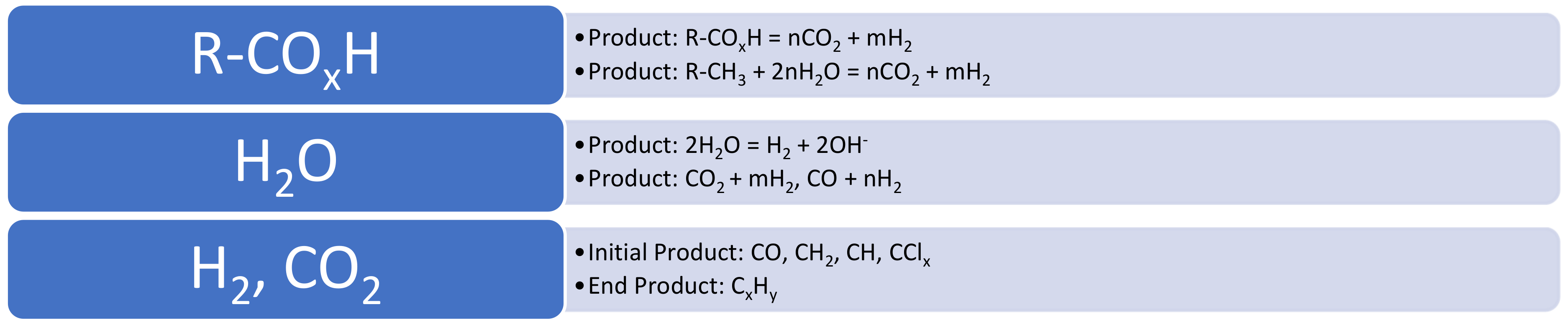
The Group 3 approach requires the ZVI to adopt the characteristics of a “Smart Material” [8], where the ZVI simultaneously undertakes the following reactions: (i) degradation of the soluble and miscible organic species in the water to CO2; (ii) production of hydrogen; (iii) hydrogenation of CO2 to produce hydrocarbons; and (iv) auto-reduction of the ZVI with H2 to ensure no loss of degradation activity (Figure 1).
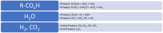
Figure 1.
Simultaneous reaction functions of the ZVI in this study.
This parallel set of reactions will result in a primary product of H2, the consumption of H2O, the consumption of [A], and a CxHy end product (Figure 1).
For example, the removal of ethanoic acid by complete oxidation with H2O (Equation (3)) will produce a gas with a 1CO2: 2H2 ratio (2 moles CO2 + 4 moles H2/mole ethanoic acid). Similarly, the removal of toluene will produce a gas with a 1CO2: 2.5H2 ratio (7 moles CO2 + 18 moles H2/mole toluene); and the removal of octane will produce a gas with a 1CO2: 4.25 H2 ratio (8 moles CO2 + 34 moles H2/mole octane). The removal of the CO2 within the water, as one or more of HCO3−, CO32−, HCO2−, [NaHCO2], NaHCO3], [H2CO2], [H2CO3], will result in an increase in the CO2: H2 ratio.
The ZVI, used in this study is constructed using four active components: m-Fe0, m-Cu0, m-Al0, and NaCl. The m-Fe0 is used as the principal active reaction component. The function of the m-Cu0 and m-Al0 are to act as promoters to increase the forward rate constant (kf) for hydrocarbon and hydrogen formation. Their presence is also intended to increase the probability of obtaining a suite of hydrocarbon products in the propyne to nonane range.
The function of the NaCl is threefold: (i) the presence of Na+ ions is used to decrease the probability of producing methane to ethane, and increase the probability of producing propane and butane; (ii) the presence of Na+ ions is used to increase the rate constants for both hydrogen production and hydrocarbon formation; (iii) the presence of Cl− ions is intended to facilitate the formation of active hydrocarbon producing sites.
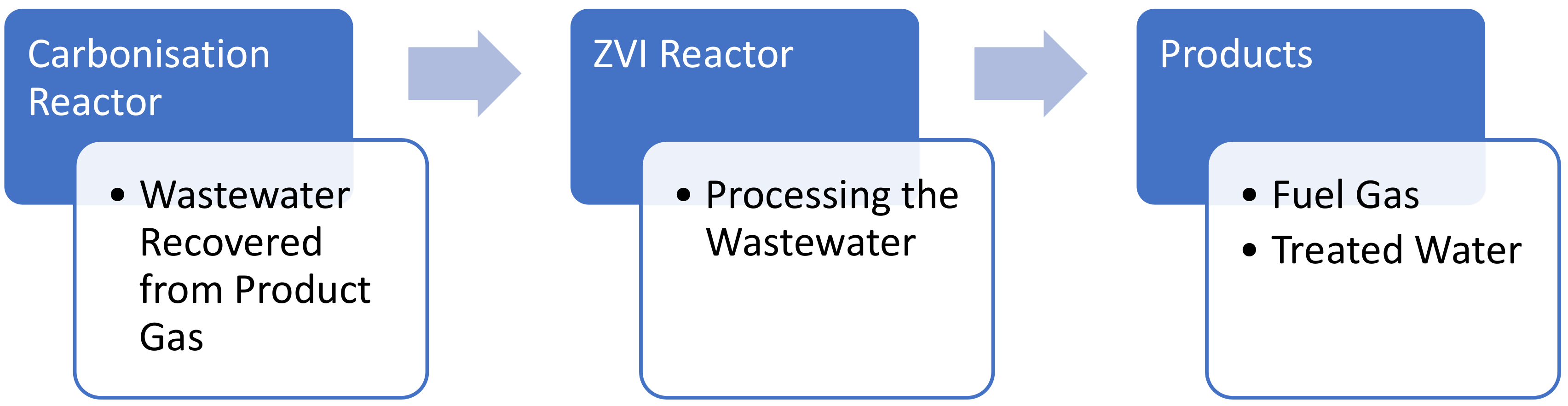
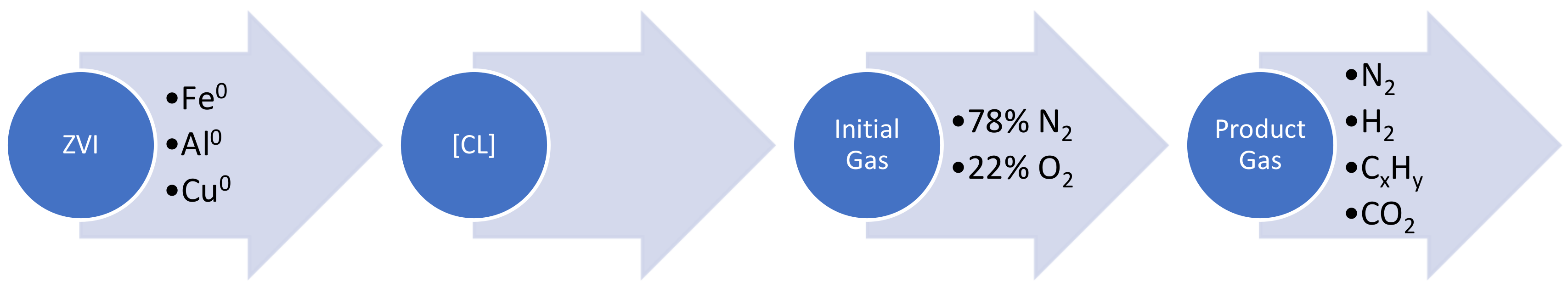
The conceptual water treatment process flow, which this study seeks to address, is summarized in Figure 2. The wastewater is generated by the operation of a carbonization reactor. This water is then processed in a ZVI reactor to produce a fuel gas product, as well as a treated water product.

Figure 2.
Conceptual process flow diagram for the ZVI process.
2. Materials and Methods
2.1. [CL], Catalyst and Retort
The organic rich water, containing [A], used in this study is a carbonisation liquid [CL] (Table 1). The [CL] was produced as a wastewater, and a condensation product (condensed at <303 K). The [CL] was condensed from the product synthesis gas, produced by an internally heated carbonisation retort [30] (Figure 2). This retort processed mixed municipal waste to produce a char and a synthesis gas ([40–48% N2] + [1–12% CO] + [10–25% H2] + [4–12% CO2] + [0–18% CH4)].

Table 1.
Example carbonization liquid [CL] (organic molar) composition from a carbonization reactor processing municipal waste (wood, plant waste, plastics, paper, carboard, organic waste). Organics represent between 10 and 50% of the molar wastewater [CL] composition.
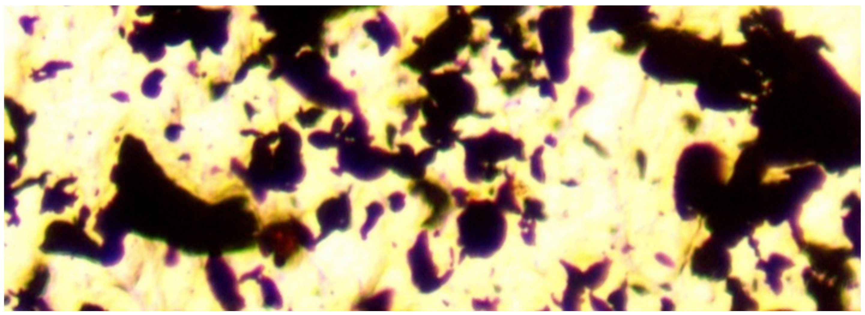
The [CL] was placed in a sealed, tubular retort (containing a Shimadzu septum for injection gas sampling), with the following volume constraints: 1 [CL]: 1.3 air. The [CL] contained: 40 g NaCl L−1 + [zero valent metal (ZVM) comprising: 181 g m-Fe0 L−1 (Figure 3) + 27 g m-Cu0 L−1 (Figure 4) + 29 g m-Al0 L−1 (Figure 5)]. The nominal ZVM particle size range was: 0.002–0.08 mm. The NaCl (halite) and m-ZVM were purchased from Wickes Ltd., Perth, UK, and MB Fibreglass, Newtownabbey, UK. The conduits, valves, and fittings were purchased from Wickes Ltd., Perth, UK and Screwfix Ltd. Perth UK. The gas pressure meters, and septa used were purchased from Cole Parmer Instruments Ltd., Saint Neots, UK.
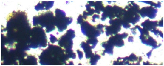
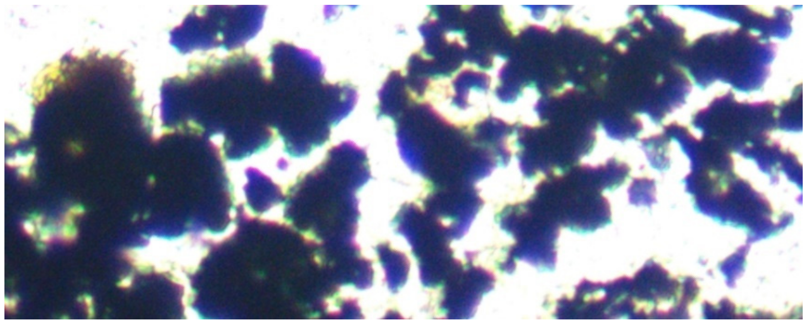
Figure 3.
Fe0 particles. Transmitted light, field of view = 0.1 mm (100 microns).
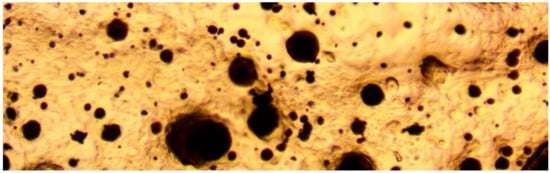
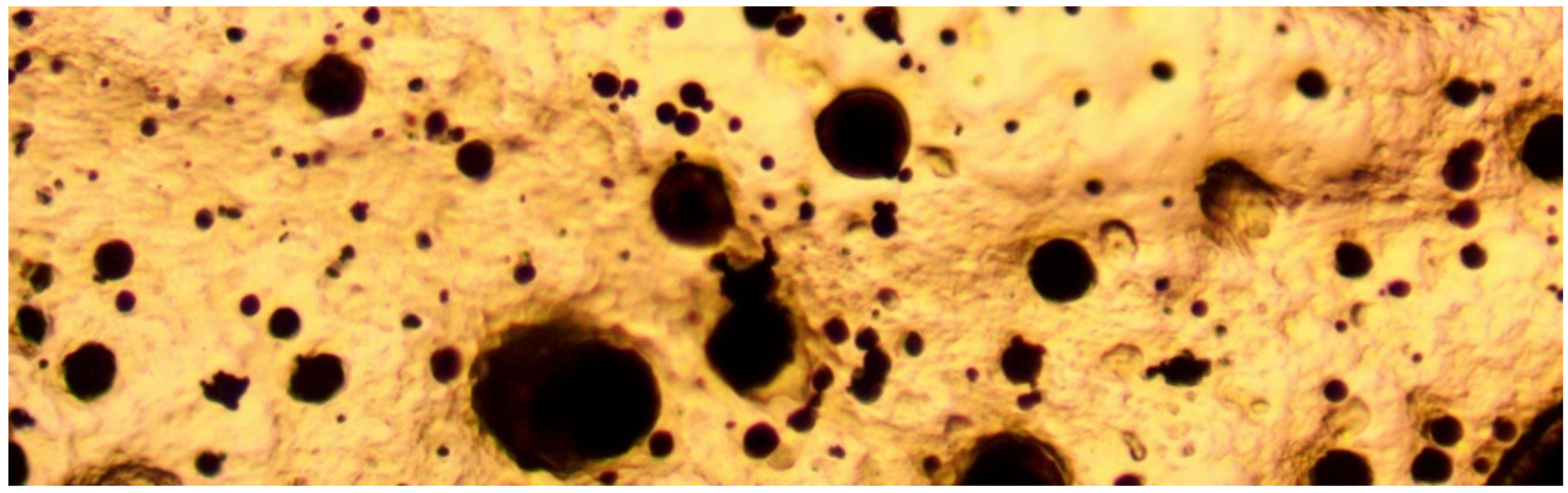
Figure 4.
Cu0 particles (dark color), embedded in resin to demonstrate the multi-modal size distribution. Transmitted light, field of view = 0.1 mm (100 microns).
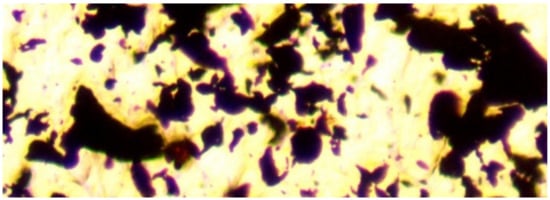
Figure 5.
Al0 particles. Transmitted light, field of view = 0.1 mm (100 microns).
Appendix A.1 provides a summary of the rationale used to select the ZVM composition used in this study.
A ME580TWB-PZ-2L-14MP dual light (reflected and transmitted light), trinocular, polarizing, metallurgical microscope ((×40 to ×2000) incorporating a 14 MP digital camera (14 MP Aptina color CMOS model MU1400-204)) was used in this study, to examine the ZVM (Figure 3, Figure 4 and Figure 5). The microscope and camera were branded by Amscope Inc., Irvine, CA, USA, and supplied by United Scope (Ning Bo) Co Ltd. Zhejiang, China. The microscope is a BH200M Series unit manufactured by Ningbo Sunny Instruments Co. Ltd., Zhejiang, China. The camera was linked to an Amscope x64, 3.7.13522.20181209 (version date: 20/9/2018) digital microscope software package (branded by Amscope, Irvine, CA, USA). This software package was used to analyse the microscope slides and resin blocks. Calibration slides were used to scale the digital microscope image:
- divisions at 0.15 mm, 0.1 mm, 0.07 and 0.01 mm supplied by No. 1 Microscope Wholesale Store, Henan, China.
- divisions at 0.01 mm supplied by United Scope (Ning Bo) Co Ltd. Zhejiang, China.
2.2. Retort Operation
The [CL] and mixed ZVM (Figure 3, Figure 4 and Figure 5) were placed in the retort. The sealed retort was left to stand for 24 h (h), at T = 273–298 K (Figure 6). The ZVM gravity differentiated as it settled to initially produce a layer of Cu0, overlain by a layer of Fe0, which was overlain by a layer of Al0. This provided a [CL]: [Al0] contact between the liquid and the ZVM body.
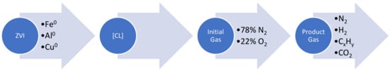
Figure 6.
Conceptual process flow within the ZVI retort over 24 h.
The retort was operated as a sealed, batch-flow static diffusion reactor. The reactions within the retort resulted in auto-pressurisation, due to gas production.
Appendix A.1 provides the rationale for using a batch-flow static diffusion reactor in preference to a continuous flow reactor.
2.3. Gas Sampling
After 24 h, the product gas composition (Figure 6) within the sealed retort was sampled using a syringe through a Shimadzu septum (purchased from Cole Parmer Instrument Co. Ltd., Saint Neots, UK). The product gas was analysed using an SRI Instruments Inc. thermal conductivity detector (TCD) gas chromatograph (GC) (purchased from Cole Parmer Instrument Co. Ltd., Saint Neots, UK). Calibration standards were purchased from BOC/Linde, Glasgow, UK. Operating conditions: start temperature: 283 K; ramp temperature: 20 K/minute; stable temperature: 523 K; run time: 2 h for C9Hx analyses (40 min to obtain molar concentrations of: H2, N2, CO, CO2, CH4, C2Hx, C3Hx, C4Hx, C5Hx, C6Hx); carrier gas = He; syringe gas sample size = 0.7 cm3.
The GC was linked to a PC, running the SRI Instruments Ltd. (Torrance, CA, USA), Peak Simple software, version 4.88.
2.4. Oil Sampling
Following the gas analysis, the retort was depressurised, and the product gas was replaced with air. The retort was agitated to fluidise the ZVM for 5 min. The ZVM was allowed to rest for 2 h before being examined for any displaced, light (low density (<1 g L−1)) immiscible liquids resting on the [CL] surface. Any immiscible liquids present at this point were sampled by syringe, and analysed in the GC. Syringe liquid sample size = 0.01 cm3.
2.5. Control Analyses
Each [CL] was placed in the retort for 24 h, before the NaCl, and zero valent metal (ZVM) was added. The gas was analysed prior to the addition of NaCl and ZVM. Only N2 was observed. Each [CL] contained no immiscible liquids, at the onset of the trial.
2.6. Pressure and Product Gas Volume Determination
The retort’s internal volume, Vr, remained constant during the reaction period. The initial number of gaseous moles in the retort at time t = 0 was Mt=0. The number of gaseous moles in the retort at time t = n was Mt=n. If the initial pressure is Pi, then at a constant temperature, the pressure at time t = n, Pt=n, is defined by Equation C1, Table 2.
Table 2.
Pressure, reactant quotient and rate constant equations. Na = N2(concentration in air)t=0; Nb = N2(concentration in the product gas)t=n; Mpt=n = moles of product in the gas body, at time t = n; MZVM = Mass of ZVM in the retort, g L−1; tr = trial duration, seconds, s; R = gas constant, J T−1 mole−1; T = temperature, K; Ea = activation energy, J mol−1, A = Avogadro’s number.
Nitrogen is assumed to be inert. If the number of the moles of nitrogen in the retort at time t = n is the same as the number of moles of nitrogen in the retort at time t = 0, then the implied pressure [P] of the sealed retort (MPa) at time t = n is defined by Equation C2, Table 2.
The analysis assumptions are: (i) the molar volume of the gas in the retort at time t = 0, is 0.05889 moles; (ii) the molar volume of nitrogen in the retort at time t = 0 is 0.0453 moles; (iii) Pi at time t = 0 is 0.1 MPa.
At time t = 0, the gas within the retort contains 78% N2 + 22% O2. If a product gas at time t = n contains 0.078% N2, then [P] = 1 MPa. When [P] = 1 MPa, the retort holds 0.5889 moles of product gas, including 0.05889 moles N2.
2.7. Partial Pressure Determination
In an aqueous environment, the forward direction of equilibrium reactions, and the water Eh, is a function of the partial pressures of specific gas components [14].
The partial pressure of H2, CxHy(g), and COx, were determined, using Equations C3 to C5, Table 2.
2.8. Reaction Quotient
A reaction (Equation C6, Table 2) has a reaction quotient, Q, which is defined by Equation C7, Table 2 [31]; where [A] and [B] are reactants, [C] and [D] are products (Equation C6, Table 2); a,b,c,d are the stoichiometric reaction requirements (Equation C6, Table 2); and e,f,g,h, are the molar concentrations of the reactants and products within the reaction environment (Equation C7, Table 2). At equilibrium, e=f=g=h [31]. Q = the equilibrium constant, Kc, when the reaction is at equilibrium [31]. The reaction moves in a forward direction when Q < Kc [31]. When the [CL] is placed in the retort, Q = Kc.
2.9. Driving the Reaction Forward
Q can be altered by one or more of the following: altering the Eh and pH of the water [14]; changing the availability of one or more reactants [31]; and removing one or more products from the reaction environment (Equation C7, Table 2) [31]. The most effective way of driving the reaction forward is to increase [h] while reducing [e] (Equation C7, Table 2).
Gaseous products forming in the ZVM collect to form gas bubbles (Figure 7). When the bubbles achieve sufficient buoyancy, they are expelled from the ZVM (Figure 7). The expelled gas bubbles rise through the [CL], before accumulating in the overlying gas body. This process reduces both [e] and Q.
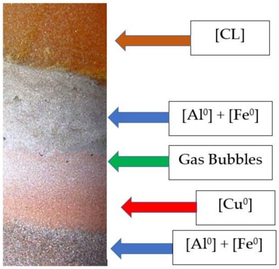
Figure 7.
Example of a [CL]: ZVM interface showing gas bubbles encased in ZVM rising into the [CL] from the ZVM body. The ZVM body shows multiple layers of gravity separation with the heavy Cu0 layers gradating upwards into a mixed Fe0:Al0 layer. Gas bubbles develop within the ZVM Bed at the junction between the Cu0 dominated zone and the Fe0:Al0 dominated zone. Field of view width: 1 cm; retort casing changed, for this example, to glass (to allow photography).
2.10. Rate Constant
The forward rate constant, kf, is measured [31] using Equation C8, Table 2. The units of kf are mole product g−1 ZVM s−1. The measured forward rate constant varies with temperature, in accordance with Equation C9, Table 2.
If kf is known (measured) for ZVM with a specific particle surface area, as, (m2 g−1); and a specific value of MZVM, then, if the ZVM particle surface area or its concentration is changed, the expected new value of kf, termed kfn, can be estimated [2] using Equation C10, Table 2.
2.11. Statistical Data Analysis
The statistical analysis of the data was undertaken using the statistical functions in MS Excel 2019. The coefficient of determination and the regression equation parameters were determined using the MS Excel 2019 (Microsoft Office, build version 2205; 15225.20204), Trendline Function. The statistical data were interpreted in accordance with British Standard BS2846 Parts 1 to 7, Statistical Interpretation of Data, BSI Handbook 25 [32].
The data used in this study are provided in the Appendix B, Figure A1, Figure A2, Figure A3, Figure A4, Figure A5, Figure A6, Figure A7, Figure A8, Figure A9, Figure A10, Figure A11, Figure A12, Figure A13, Figure A14, Figure A15, Figure A16, Figure A17 and Figure A18.
3. Results
3.1. Initial Test
An initial experiment (24 h duration) was undertaken to determine whether CxHy could be produced in significant quantities. The [CL] used in the experiment was Example 3, Table 1.
The molar product gas composition was: N2 = 33.56% (1 L); H2 = 21.6% (0.62 L); and hydrocarbons = 44.84% (1.34 L). The reactor pressure, calculated using Equation C2 (Table 2), after 24 h, was 0.223 MPa.
The hydrocarbon component of the product gas comprised as follows: propyne = 0.11%; propene = 5.3%; n-propane = 14.25%; n-butane = 18.94%; n-pentane = 5.44%; n-hexane = 0.45%; and n-heptane = 0.17%.
The presence of hydrogen is consistent with a Group 2, or Group 3 reaction mechanism. The implied hydrogenation (Group 2) reactions and related reaction quotients are provided in Table 3 and Table 4. The absence of CO2 in the product gas indicates that either all of the produced CO2 was consumed during a Group 3 reaction; or that the hydrocarbons were produced by a Group 2 reaction.
Table 3.
CxHy Formational equations implied by product gas compositions. The Equations 1 to 9 are Group 2 reactions, which assume that ethanoic acid and propionic acid form alkanes as a direct degradation product. Equation 10 is alkane production using the Group 3 reaction where the gas feed stock is CO2. Equations 11 and 12 provide the aqueous degradation reaction for ethanoic acid to form carbonic acid and CO2. ΔHf(298K) = heat of formation for the reaction at 298 K, P = 0.1 MPa; ΔGf(298K) = Gibbs free energy for the reaction at 298 K, P = 0.1 MPa. ΔHf(298K) and ΔGf(298K) calculated using the methodology defined by [31], and the data sources defined in Appendix A.4.
Table 4.
Group 2 reaction quotient equations. Subscripts [i, j, k, l, m] are molar concentrations of products and reactants. The equations are constructed using the methodology defined in [31].
3.2. Statistical Trials
The initial trial results raised four questions:
- Why was no CO2 observed in the product gas? Was this because all of the required hydrogen was sourced from the oxidation of Fe0?
- Why were the hydrocarbon yields >7 orders of magnitude greater than those previously recorded [15]? Was this because the required hydrogen and CO2 were sourced from the oxidation of organic species [A]?
- Are the results repeatable?
- Do the product composition results change if the temperature is increased?
The initial experiment, was followed by a series of repetition experiments, undertaken at T = 273–298 K (duration = 24 h, n = 100), and at T = 348 K (duration = 10 min, n = 12). These repetition experiments sought to provide answers to each of these questions.
- At T = 273–298 K, four product outcomes were observed:
- ○
- Outcome 1: H2 + no alkanes, or no H2 + no alkanes (29% of outcomes);
- ○
- Outcome 2: H2 + gaseous alkane and no liquid alkanes (12 % of outcomes);
- ○
- Outcome 3: H2 + liquid alkanes and no gaseous alkanes (29% of outcomes).
- ○
- Outcome 4: H2 + gaseous alkanes + liquid alkanes (30% of outcomes).
- At T = 348 K, the four product outcomes were:
- ○
- Outcome 5: 36.7% CO2, and no alkanes, or H2 (8% of outcomes);
- ○
- Outcome 6: H2, CO2, and no alkanes (16% of outcomes);
- ○
- Outcome 7: H2 + gaseous alkanes and no CO2 (25% of outcomes);
- ○
- Outcome 8: gaseous alkanes + CO2 + H2 (50% of outcomes).
Outcomes 5, 6, and 8 indicated that CO2 was produced as part of the Group 3 process. The absence of CO2 in Outcomes 1, 2, 3, and 4, could be interpreted as indicating that the majority of the hydrocarbons were formed using a Group 2 process. Alternatively, these outcomes could be interpreted as indicating that incomplete oxidation of the organic species had occurred, and any CO2 produced had been consumed within a Group 3 process.
Outcomes 2,3,4, 7, and 8 indicate that alkanes are only present when hydrogen gas has been produced. This is consistent with both Group 2 and Group 3 processes.
Outcome 5, when viewed in the context of the other Outcomes, indicates that the absence of CO2 in Outcomes 1, 2, 3, 4, and 7, may result from CO2 hydrogenation (a Group 3 process).
3.2.1. Gaseous Results at 273–298 K
Alkane product compositions are summarised in Table 5. For each gas species, kf increases with increasing [P]. A marked change in the rate of change of kf with [P] occurred when [P] exceeded 0.2 MPa (Table 6).
Table 5.
Composition of the gaseous products, where T = 273–298 K. n = 42.
Table 6.
Rate constant for the gases in Table 5. Ln kf = [a] Log [P] + [b], where [a] and [b] are regression constants. R2 = coefficient of determination.
3.2.2. Liquid Results at 273–298 K
The molar composition of the immiscible liquid is provided in Table 7. The bulk of the weight in the liquid is in the C7 to C9 range.
Table 7.
Molar composition of the clear liquid hydrocarbon. n = 57.
3.2.3. Gaseous Results at 348 K
The average gas composition was: 31.02% N2 + 9.69% CO2 + 45.89% H2 + 14.58% CxHy.
The hydrocarbon component of the product gas comprised as follows: propyne = 11.15%; propene = 27.45%; propane = 17.21%; butane = 19.86%; pentane = 21.71%; hexane = 1.76%; and heptane = 0.73%. The associated rate constants are provided in Table 8.
Table 8.
Rate constant for the gases produced at 348 K. Ln kf = [a] Log [P] + [b], where [a] and [b] are regression constants. R2 = coefficient of determination. n = 12.
4. Discussion
4.1. Hydrogen
Significant quantities of hydrogen were generated in the experiments. This hydrogen was used to:
- (i)
- remove O2 from the [CL] and the gas body;
- (ii)
- saturate the [CL] and gas body;
- (iii)
- participate in the remediation reactions;
- (iv)
- pressurise the retort.
4.1.1. Removal of O2 from the [CL]
A portion of the H2 generated, Hd1, reacted to remove O2 dissolved in the [CL]. A further portion of the H2 generated, Hd, remained dissolved in the [CL]. This volume can be estimated from Henrys law (Table 9, Equation H1).
Table 9.
Equations used to interpret the observed hydrogen. Hfh = moles of free hydrogen (measured); Hc = moles of free gaseous alkanes (measured); Ho = moles of hydrogen required to remove the O2 (measured); f = number of moles of H2 required to produce 1 mole of gaseous alkane (Table 5). The forward rate constant, kfh, is provided in Table 6. kcf = moles product g−1 ZVM s−1 MPa−1; ΔP = driving force, MPa. Ag = moles of gaseous alkane in the product gas.
4.1.2. Removal of O2 from the Gas Body
Initially, H2 entering the gas body will remove O2(g) (Table 9, Equation H2). During this initial phase, the retort depressurises from 0.1 MPa to 0.078 MPa. Once the O2 has been removed from the gas body, additional H2 entering the gas body results in a gas body containing H2 + N2. This gas flow increases the gas pressure in the retort, and increases the availability of dissolved H2 within the [CL].
4.1.3. Removal of H2 to form Alkanes
The removal of hydrogen to form an alkane (Table 3, Equations 1 to 10) will reduce the rate of pressure increase in the retort, by consuming hydrogen to form the alkane. The total amount of hydrogen generated, Hgh, determined in moles (Table 9, Equation H3), as a function of the amount of free hydrogen, and the hydrogen consumed to manufacture the alkanes. The forward rate constant for the produced hydrogen, kfHgh, is expressed in moles of H2-produced g−1 ZVM s−1 for T ≤ 298 K, and is defined in Table 9, Equation H4.
4.1.4. Impact of the Driving Force Created by H2 on Hydrocarbon Formation Rate Constants
The forward rate constant, kf, (moles product g−1 ZVM s−1) can be expressed in terms of the general flux equation [33] (Table 9, Equation H5). The volume of the reacting gas, Vrg, in moles, is defined by Equation H6, Table 9. The volume of the product gas, Vpg, in moles, is defined by Equation H7, Table 9. The pressure associated with the reacting gas Prg, MPa, is defined by Equation H8, Table 9. The driving force created by the reaction is defined by Equation H9, Table 9.
Table 10 provides the forward rate constants, kf, for the formation of each gas [moles gas g−1 [ZVM] s−1] as a function of ΔP.
Table 10.
Rate constants for the gases in Table 6. Ln kf = [a] Log [ΔP] + [b], where [a] and [b] are regression constants.
4.2. [CL] Redox Regimes
The [CL] contains three separate redox regimes, which define the stable oxidation number of hydrogen at different locations within the [CL] column. The boundary constraints are defined in Table 11. The ZVM Bed, during alkane production and catalyst activation, is in Stability Field 2. The initial stability field for the [CL], when it is placed in the reactor, is termed Stability Field 0. The bulk of the [CL] is in Stability Field 1 during the reaction period.
Table 11.
Redox (Eh:pH) stability field regimes in the [CL]. The Eh of the upper boundary of Stability Field 2, decreases with increasing pressure, and decreases with the increasing availability of H+ and OH−. In a Nernstian, or Faradaic reaction, basic chemistry [14,31] defines: Eh, volts as Eo–(0.0591(nH+/ne−))pH + (0.0591/[ne−])Log((moles or partial pressure product/moles or partial pressure reactant); Eo = Standard reduction potential for the reaction; Eo is available for most reactions, in standard data books of electrochemical series. The sources of Eo used in this study, are provided in Appendix A.4. By definition, the Eo value for H2 is 0. Partial pressures can be defined in atmospheres [14,31]. In this study they are defined in MPa, where 1 atmosphere pressure = 0.1 MPa. The required adjustment to the standard Nernstian equation, where partial pressures are in MPa, is provided in this table.
4.2.1. Hydrogen Sources within Each Stability Field
Hydrogen (Table 11) is derived from three sources: redox interactions, ZVM oxidation by water, and ZVM catalysis of the water and [CL]. When the ZVI is first placed in the water, it is placed into Redox Stability Zone 0 (Table 11). The Fe0 modifies the water Eh and pH by saturating the water with H2(g,aq) (Figure 7) and OH− ions (Table 11). These modifications have the effect of both increasing pH, and decreasing Eh [14].
4.2.2. Iron Reactions within Each Stability Field
In most Group 1 processes, the water remains within Stability Field 0, or may transition during the course of the water treatment from Stability Field 0 to Stability Field 1. All Group 2 and Group 3 processes are undertaken within Stability Field 1 and Stability Field 2. The associated Fe0 reduction and oxidation reactions are provided in Table 12.
Table 12.
Fe0 reactions, catalysis, and catalyst formation within the different redox stability fields. Catalyst formation occurs in Stability Field 1 and Stability Field 2.
4.2.3. Carbon Sources within Each Stability Field
The Group 2 reaction of direct alkane production from carboxylic acids by hydrogenation could occur in Stability Field 1 (Table 2 and Table 3). When the alkanes are formed by a Group 3 process, the carboxylic acids are first degraded to CO. The reactions required to degrade the carboxylic acid to CO are summarised in Table 13. The Group 3 approach requires the convection counter-current, created by gases rising from the ZVM Bed (Figure 4), to draw fluids from the [CL] (Stability Fields 0 and 1) into the ZVM Bed (Stability Field 2).
Table 13.
Fe0 degradation of carboxylic acids in the different stability fields. The Eh associated with the gaseous stability transition from CO to CO2, given by the reaction: CO + H2O = CO2 + 2H+ + 2e−.
4.2.4. The ZVM Redox Environment
Zero valent metals have an Eh on their surface, which is defined by the transition to an ion, an oxide, or an oxyhydroxide [14]. All of the metals, Fe0, Al0, and Cu0, are stable in Stability Field 2, in both their zero valent metal form, and their hydride form (FeH2, AlH3, CuH). Cu0 is stable as Cu0 within the Stability Field 1, and much of Stability Field 0 [14]. Al0 and Fe0 oxidise and ionise in Stability Field 0 and Stability Field 1 [14]. The production of alkanes from CO requires the catalyst to be held within Stability Field 2 (Table 13).
The Eh:pH relationships and associated reactions within a ZVM Bed, held in Stability Field 2 (Table 14), indicate that the Eh, on some of the catalyst surfaces, will be <−1.5 Volts.
Table 14.
Eh relationships within the ZVM Bed.
The metals within the ZVM Bed (Table 14) operate as separate electrochemical cell electrodes, which are separated by an electrolyte [CL]. The cells are: Cu0:Al0, Cu0:Fe0; and Fe0:Al0. This structuring facilitates the catalytic formation of H2(g) at the dihydride catalytic sites ([FeH2], [Fe5C2]H2), or the trihydride catalytic site ([AlH3]), (Table 12). The operation of this cell is shown in Figure 7, where hydrogen gas bubbles grow within the ZVM Bed, at the [Cu0:Al0, Cu0:Fe0] interface.
4.3. Formation of Alkanes
The placement of Cu0:Fe0 in Stability Field 2 in the presence of H− and CO will create two types of activated catalyst: (i) a dihydride, [FeH2] and [Fe5C2H2]; and (ii) a monohydride [H[Fe5C2]] (Table 15). The dihydrides are hydrogen formation catalysts, but can inter-react to form a monohydride carbide catalyst (Table 15). All three types of activated catalyst may be involved in alkane formation, using an alkyl mechanism (-CH2-) [34]. It is more likely that the dihydrides will preferentially catalyse hydrogen formation (Table 15).
Table 15.
Alkane formation reactions in Stability Field 2: alkyl chain growth mechanism.
4.4. Formation of Alkynes
The Group 3 chain growth mechanism in Table 15 assumes an alkyl insertion mechanism, where the alkane chain grows by the addition of -CH2- units. The presence of propyne in the product mix suggests that chain growth involves an alkylidyne insertion mechanism [34]. In this mechanism, the chain grows by the insertion of -CH- units (Table 16). The basic growth unit on the catalyst surface is [C1H] (methylidyne). The simple generic reactions on the catalyst surface are:
Table 16.
Chain growth using an alkylidyne mechanism to produce propyne.
Step 1 formation of acetylene on the catalyst surface:
[C1H] + [C1H] = C2H2(ads),
Step 2 formation of propyne by the addition of an alkyl unit:
([C1H] [C1H])(ads) + [CH2] = C3H4(g),
The requirement for an alkylidyne mechanism to produce propyne provides further evidence that the hydrocarbons were produced through Fe0 catalysis. This is reinforced by the rate constants, which indicate that propyne production disproportionately increases with both increasing pressure and increasing temperature.
4.5. Role of Chlorine Ions in the Formation of Alkynes, Alkanes and Alkenes
Chlorine ions can participate in hydrocarbon formation [35], where:
[CO2] + 3Cl− + 2H2 = [CCl3−] + 2H2O + 2e−,
[CCl3−] + CO2 + 4H2 = [[CCl2] [CH3]]− + HCl + 2H2O + 8e−,
[[CCl2] [CH3]]− + CO2 + 5.5H2 = [CH3][CH2] [CH3]] + 2HCl + 2H2O + 8e−,
This type of reaction may have resulted in the hydrocarbon products identified by Fogel [20].
4.6. Role of Na+ Ions
In Stability Field 0 and Stability Field 1, Na is present as Na+ ions. In Stability Field 2, it forms a monohydride, NaH [14].
Within the retort, there is a fluid circulation pattern, where fluids, displaced by rising gases from the ZVM Bed (Stability Field 2) rise to Stability Field 0. A counter current in the [CL] moves fluids from Stability Field 0 into Stability Field 2 in order to replace the expelled fluids.
Na+ ions arriving in Stability Field 2 will react to form NaH [14] (Equation N1, Table 17). NaH(aq) arriving from the ZVM Bed into Stability Field 1 will decompose to release H0 (Equation N2, Table 17). NaH(aq) arriving from the ZVM Bed into Stability Field 0 will decompose to release H+ [14] (Equation N3, Table 17).
Table 17.
Reactions of Na+ ions in different Stability Zones.
This non-catalytic circular process may play a major role in transporting hydrogen from the ZVM Bed to the gas body.
Role of Na+ Ions in CO Formation
The reactions in Table 15 and Table 16 require the presence of CO in Stability Field 2. This will naturally form as a result of redox reactions (Table 13), as fluids (from Stability Field 1 and Stability Field 0) are circulated into Stability Field 2.
A complicating factor is that Na+ ions contained in Stability Field 0 will react with H2CO3 to produce [NaHCO3] (Equation N4, Table 17). The transport of the [NaHCO3](aq) into Stability Field 1 will result in disassociation (Equation N5, Table 17). The transport of the [NaHCO3](aq) into Stability Field 2 will result in disassociation, CO formation, and hydride formation (Equation N6, Table 17).
The fluid circulation process within the retort provides a carrier mechanism, whereby carbonic acid can be delivered from the [CL] to the ZVM Bed, as CO, and [H−] contained within the ZVM Bed can be delivered to the [CL] and gas body as H2.
4.7. Anderson Schulz Flory Distribution
Group 3 alkane products can follow an Anderson–Schulz–Flory (ASF) distribution [15], where:
Cn = (1−α) αn−1,
Cn = mole fraction of an alkane with a carbon number of n; α = the probability growth factor:
α = Rp/Rp + Rt,
Rp = rate of propagation; Rt = rate of termination.
4.7.1. Alkane Formation as a Function of P, at T ≤ 298 K
The rate constants for kfC3 to kfC7 allow the molar gas composition and volumes to be defined as a function of pressure and carbon number (Table 18).
Table 18.
Production of light hydrocarbons as a function of auto-pressurization of the reaction environment. Production volumes and energy values are standardized to a reactor train, retort size comprising 1 m3 [CL] + 1.3 m3 gas. T = <298K.
4.7.2. α Values for Alkane Formation as a Function of P, at T ≤ 298 K
The molar compositions in Table 18 allow the ASF α values to be defined (Table 19) as a function of pressure and carbon number. These values can change as a function of carbon number, catalyst selectivity, temperature, and pressure [36,37,38].
Table 19.
ASF α value as a function of pressure for the gaseous hydrocarbons (Table 18).
4.7.3. Analysis of Liquid Alkanes
The oils have high ASF α values, which vary with carbon number (Table 20). The recovered liquids were obtained by depressurising and fluidising the ZVM Bed. This may indicate that, prior to the fluidisation, these alkanes were still attached to their catalytic sites.
Table 20.
ASF α value for the liquid hydrocarbons.
Under this interpretation, alkane release from a catalytic site may only occur when the particles are agitated, or moved by rising gas (H2) bubbles.
4.7.4. Impact of Increasing Temperature
The gas analyses at T = 348 K (Table 10) indicate (Table 21) that the relative abundance of each gas component increases with increasing pressure. At low pressure, CO2 is the dominant product gas. Alkane and H2 production increase at a higher rate when combined with increased pressure.
Table 21.
Relative molar abundances of the principal product gas components as a function of reactor pressure. T = 348 K.
The associated ASF α values (Table 22) are consistent at low pressures, with most of the product being retained in the ZVM Bed, while at high pressures, the high level of hydrogen discharge results in short chain alkane discharge to the gas body.
Table 22.
ASF α value as a function of pressure for the gaseous hydrocarbons (Table 21).
4.8. Group 2 Process
If the alkanes were produced by a Group 2 process, then the product gas should have contained a high molar ethane:propane ratio, in order to reflect the relative ratio of the source acids (ethanoic acid: propionic acid) in the [CL] (Table 1).
The absence of ethane may suggest that the alkanes result from a mixture of a Group 2 and Group 3 processes, or that the bulk of alkane production is a result of a hybrid Group 3 process, where:
H[Fe5C2] + CH3COOH + 4H− = [H[Fe5C2][CH]2[CH]2]+ + 2H2O + 2e−
H[Fe5C2] + CH3CH2COOH + 4H− = [H[Fe5C2][CH]2[CH]2][CH2]+ + 2H2O + 8e−
This hybrid interpretation would allow the generic Group 2 equations (Table 3 and Table 4) to describe alkane formation. An alkylidyne mechanism (Table 16) would still be required to produce propyne. This hybrid process appears to be a simple compromise interpretation, which could explain the observations, and, if operative, would work in parallel with both the alkyl and alkylidyne Group 3 mechanisms (Table 15 and Table 16).
4.9. Continued Chain Growth
The experiments of both [Hardy and Gilham [15]] and [Fogel [20]] demonstrated that increasing the length of time spent in the reaction environment increased the number of carbon species present. The chain growth followed the ASF α relationship (Equation (10)) [15].
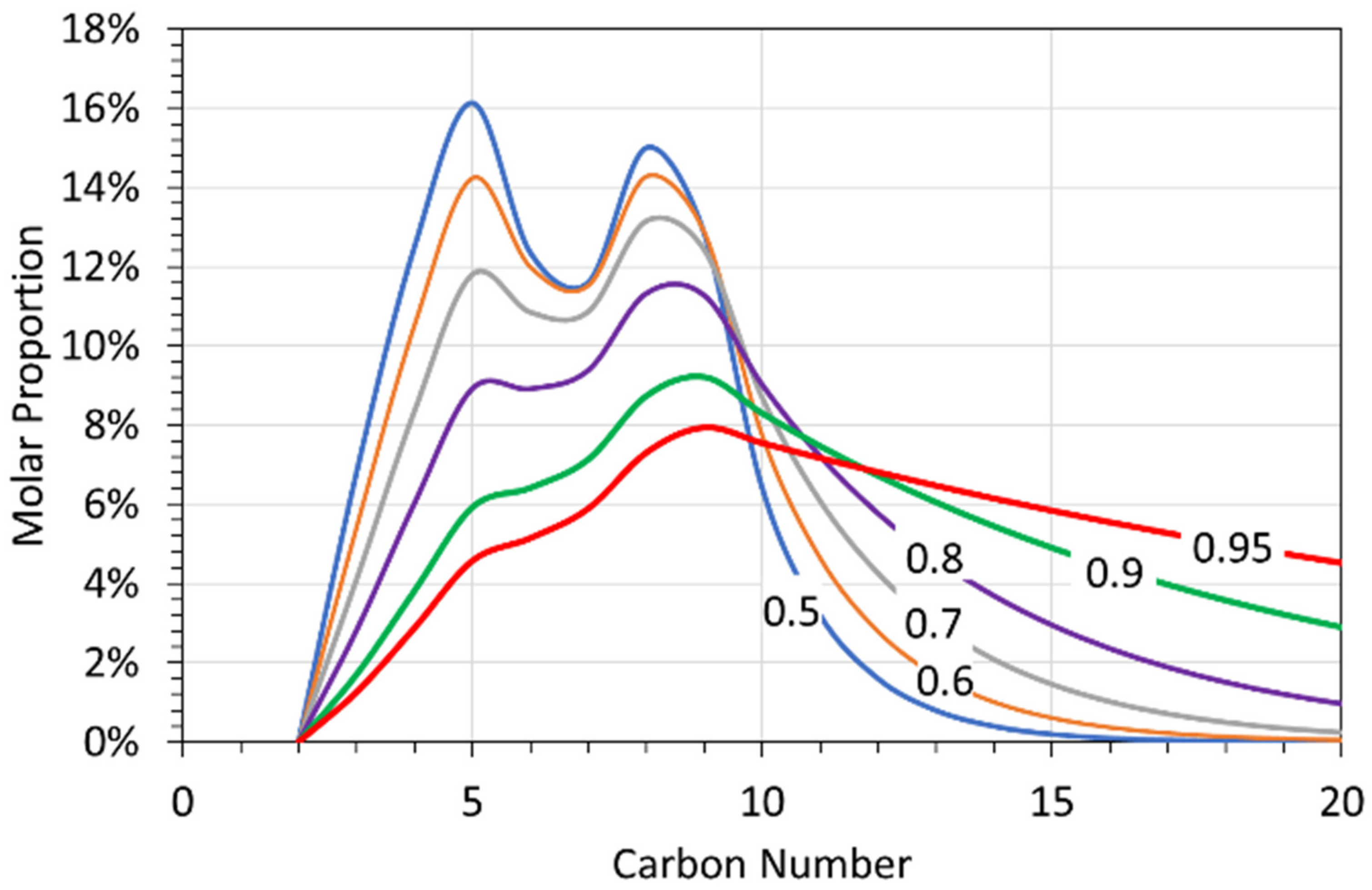
Their results [15,20] imply that the continued chain growth of the recovered oil will produce a product which can be described by an ASF α value. This chain growth (Figure 8) will create a liquid product, whose molar composition is a function of its ASF α value.
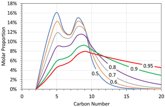
Figure 8.
Average liquid alkane composition, produced at < 298 K, where the alkanes were subsequently grown at ASF α values of 0.5 to 0.95. Blue line = ASF α value of 0.5; Brown line = ASF α value of 0.6; Grey line = ASF α values of 0.7; Purple line = ASF α values of 0.8; Green line = ASF α values of 0.9; Red line = ASF α values of 0.95; Appendix B Figure A1 gives the probability values for the alkane composition when the ASF α value is 0.0.
4.10. Potential Value of a Fuel Gas
The experiments have established that a fuel gas can be produced from the wastewater which has been condensed from the carbonization of organic matter. The fuel gas, when combusted, will produce H2O and CO2 as by-products. Table 18 and Table 21 indicate the expected fuel gas volumes, fuel gas composition, and calorific value as a function of operating pressure. These results are standardized to a retort size containing 1 m3 [CL] and 1.3 m3 gas. The residence time of the [CL] in the retort is assumed to be 24 h when T ≤ 298 K, and 10 min when T = 348 K.
The alkane weight generated at 298 K and 0.1 MPa (Table 18) was around 0.67 g L−1. The feed water had a density which ranged between 1.1 and 1.4 g cm−3, indicating the presence of between 100 and 400 g organic solutes L−1. This indicates that between 0.1% and 0.67% of the organic solutes participated in hydrocarbon formation.
Increasing the temperature to 348K resulted in the production of around 59 g L−1 of alkanes (Table 21). This indicates that between 14% and 59% of the organic solutes participated in hydrocarbon formation.
A reactor train operated at 348 K, containing 1 m3 [CL] (processing 144 m3 [CL] d−1), has the potential to produce a fuel gas (containing between 0.8 MWh d−1 and 14 MWh d−1, of thermal energy (Table 21)). The implied molar CO and feedstock consumption is indicated in Table 23.
Table 23.
Implied CO consumption, at = 348 K for a reactor containing 1 m3 [CL]. Feedstock numbers assume that 100% of the CO is produced from either ethanoic acid or propionic acid. At operating pressures of >0.5 MPa, the rate constants indicate that the frequency of [CL] replacement will be increased from 6 m3 h−1 m−3 reactor’s liquid capacity.
5. Novelty
This study has established that if an organic rich wastewater is remediated in a sealed diffusion reactor, sustained high rates of hydrogen production and alkane production can occur.
5.1. Hydrogen
Prior to commencing this study, the best reported H2 production rates for: (i) 2000–5000 nm m-Fe0 were in the range 10−8 to 10−9 g H2 g Fe0 s−1 (Table 24) [39,40]; and (ii) 60 nm m-Fe0 were in the range 10−7 to 10−10 g H2 g Fe0 s−1 (Table 24) [39]. This study has established H2 production rates of 10−4 to 10−6 g H2 g Fe0 s−1 for 2000–80,000 nm m-Fe0 when P ≤ 1 MPa (Table 24). These rates were two to four orders of magnitude higher than the previously reported hydrogen production rates. The previous studies produced the hydrogen from the oxidation of Fe0 by H2O.
Table 24.
Comparison of hydrogen production rates in this study and previous studies. P = pressure, MPa; Pw = g Fe0 L−1; kf = forward rate constant g H2 g−1 Fe0 L−1 s−1. n = a reference value for Pw. Data source for m-Fe0 + n-Fe0: [39,40]. The published m-Fe0 and n-Fe0 data [39,40] comprises (i) amount of H2 produced in a trial; (ii) amount of Fe0 used in the trial, g L−1; and (iii) trial duration, h−1. In this table, this data [39,40] has been reinterpreted, to determine a value of kf for these trials, using the methodology defined in [31].
In this study, the hydrogen was produced primarily from the oxidation of organic species to form CO2 (Table 1).
At temperatures of <298 K, the H2:C molar ratio varies between 4.4 and 4.9 (Table 18). This ratio is consistent with a Group 3 hydrocarbon formation process.
At temperatures of 348 K, the H2:C molar ratio varies between 1.2 and 1.3 (Table 21). This ratio is consistent with a Group 3 hydrocarbon formation process. H2 is calculated as [free H2] + [H2 required for hydrocarbon formation by CO2 hydrogenation].
5.2. Hydrocarbons
Prior to commencing this study, the best reported hydrocarbon production rates associated with COx hydrogenation using Fe0 catalysts were obtained at temperatures of >425 K [36]. This study used a Fe:Cu ZVI combination, and obtained production rates of 10−2 to 10−5 g CxHy g Fe0 s−1 (Table 25). These rates are >7 orders of magnitude greater than those recorded by Hardy and Gilham [15].
Table 25.
Comparison of hydrocarbon production rates in this study and previous studies. P = pressure, MPa; Pw = g Fe0 L−1; kf = forward rate constant g H2 g Fe0 L−1 s−1. Data sources [15,41,42]. Stuttgart are weight proportioned Fischer–Tropsch catalysts [41]. Trials D3001…A3218.087 are Fischer–Tropsch–Synol catalysts, receiving 1CO:1H2, and developed for use by I.G.Farben in their Leuna plant in the 1940s [42]. Catalyst D3001 contained 66.78 wt% Fe; [42]. The Stuttgart data was obtained from Table 60 of reference [41]. The other Fischer Tropsch data was obtained from Table 74 and Table 77 of Reference [41]. Data is provided in these tables as grams hydrocarbon produced per 1m3 of 1H2 + 1CO flowing through a fixed bed reactor containing catalyst. This data is not directly comparable with the data obtained in this study. To allow comparison with this study, the space velocities (volume volume−1 unit time−1) and catalyst composition information provided in reference [41] was used to estimate the weight of catalyst present in each reactor. These quantitative interpreted estimates, were then used to estimate the forward rate constants, associated with each reactor. The calculated (estimated) parameters were: (i) weight of catalyst present in each reactor, g L−1; (ii) Estimated amount of CO received, g L−1 over the reported period of measurement; (iii) Amount of hydrocarbon produced, g L−1 reactor capacity. This information was then used to estimate kf for the Fischer Tropsch reactors. The Hardy & Gilham study [15] only supplied the following information: (i) Amount of hydrocarbon produced, g; (ii) trial duration, (144 h); (iii) amount of Fe0 used, g; (iv) amount of HCO3− in the feed water mg L−1. This information has been used here to provide an interpretation of kf. It should be noted that, many ZVI reactions show a marked decline in kf, as a function of reaction duration [2]. It is therefore possible that the values for kf, based on the data in [15], may, if they had been measured after 24 h, have been an order of magnitude higher.
The carbon concentrations in the [CL] are about five orders of magnitude greater than those present in the liquids used by Hardy and Gilham [15]. The H2 concentration in the retort was many orders of magnitude higher than those used by Hardy and Gilham [15].
Therefore, the difference between the results of this study and those achieved by Hardy and Gilham [15] can be reconciled as a reflection of the differences in carbon source, carbon availability, redox environment, and hydrogen availability.
The original Fe:Cu catalysts for gas phase CO hydrogenation were developed by Professor Fischer and Professor Tropsch [41]. Their original experiments (Stuttgart trials) obtained production rates of 10−6 g CxHy g Fe0 s−1 (Table 25). These production rates are about an order of magnitude lower than those obtained in this study (Table 25), and three orders of magnitude lower than those obtained by other Fe0 Fischer–Tropsch catalysts (Table 25). The gaseous Fischer–Tropsch results (Table 25) reconcile as a function of space velocity and gas pressure, where the rate constant increases with increasing pressure and decreasing space velocity.
The results from this study are associated with a substantially lower space velocity, lower temperature, higher pressure, higher reactant availability, and a higher H2:C ratio than the Stuttgart results. These differences may have been sufficient to account for the differences between the two sets of trials if they had both produced hydrocarbons using a similar process.
5.3. Wastewater
The wastewater [CL] product volume declined during the remediation process as the water was modified to produce both hydrogen and hydrocarbons. This volume decline resulted from the process consumption of water and DOM. In some instances (associated with high H2 production), the resultant increase in the DOM:H2O ratio was sufficient to allow for the recycling of the [CL] product to the carbonization reactor. These observations indicate that it may be possible to develop a process to carbonize municipal waste (and other organic matter) without producing a wastewater product, which requires disposal to a groundwater or riparian environment.
6. Conclusions
This study has confirmed that ZVI is a multi-tasking, water-remediation agent, which has the properties of a Smart Material. The study demonstrates that ZVI can simultaneously:
- degrade organic species present in [CL] to CO2;
- degrade water and organic species to produce hydrogen;
- hydrogenate the produced carbon oxides to produce hydrocarbons.
The forward rate constant for each reaction increases with both increasing pressures and increasing temperature. These changes have three major impacts:
- the removal rate for the organic solutes contained in the water increases with temperature and pressure;
- hydrogen production increases with temperature and pressure at a faster rate than alkane production;
- carbon dioxide production, when present, increases with temperature and pressure at a slower rate than hydrogen production.
At temperatures of <298 K, 58% of trials produced no gaseous hydrocarbons. At 348 K, 25% of trials produced no gaseous hydrocarbons. The reasons why some trials produced gaseous hydrocarbons and others did not have not been elucidated, but may relate to the initial oxidation of the organic solutes.
The production rates of combustible product gas at elevated temperatures may create a potentially useable fuel gas. The observed fuel gas production rates are subeconomic, but identify that it may be possible to combine water remediation with fuel gas production.
The oxidation of organic solutes and the conversion of CO2 to alkanes, combined with hydrogen production, have been obtained by using the ZVI to stratify the Eh of the water column. This structuring has created redox zones within the water column, where the oxidation number of hydrogen is +1, 0, or −1.
This scoping study has identified a new research direction for the treatment of water which contains high concentrations of DOM. While the amount of H2, CxHy, and CO2 produced will be site specific, this study indicates that it may be possible to use ZVI to transform dissolved organic pollutants contained in wastewater to immiscible recoverable fluids (CxHy) and recoverable gases.
Funding
This research received no external funding.
Institutional Review Board Statement
Not applicable.
Informed Consent Statement
Not applicable.
Data Availability Statement
The data used in this study are placed in the tables contained within the paper, and Appendix A.
Acknowledgments
The Reviewers, and Special Issue Editor, are thanked for their incisive and thoughtful reviews, which substantially improved the paper.
Conflicts of Interest
The author declares no conflict of interest.
Appendix A
The Appendix contains the data set used in the study. It also contains a summary of the patents consulted in formulating the Fe:Cu:Al:Na ZVI combination which was used in this study.
Appendix A.1. Hydrogen Source
The required hydrogen for both Group 2 and Group 3 reactions was generated by the interaction of Fe0, Cu0, and Al0 with water [39,40]. The values of Eo used in designing the zero valent metal (ZVM) bed were: Fe = −0.447 V (Fe2+:Fe0); Al0 = −1.662 V (Al3+:Al0); Cu0 = +0.52 V: Cu+:Cu0.
Appendix A.2. ZVI Reactor Type
In a ZVI reactor, the ZVI particles are not porous, and are unsupported. Any catalytic sites are located on the particles external surface. Alkane fronds will be expected to grow from the particle surface into the adjoining water-filled, inter-particle porosity.
In a continuous-flow, fixed-bed, fluidized-bed, or slurry-bed ZVI reactor, there is a continual abrasion of ZVI particles. This abrasion would dislodge any growing alkane fronds, thereby preventing the growth of long chains, and may prevent alkane chain growth initiation.
A batch-flow, sealed, static-diffusion reactor contains a ZVI bed and a gas body, which are separated by a water body. The fluids are not agitated during the reaction period, apart from during the initial mixing. The fluid interaction between the three bodies is via diffusion during the reaction period. This quiescent ZVI bed will allow alkane fronds to grow from the ZVI particle surfaces into the adjacent inter-particle porosity.
Appendix A.3. ZVI Composition
The addition of particulate Cu0 to particulate Fe0 increases the forward rate constant, kf. [US Patent 2,626,275 (20 January, 1953); French Patent 870,679 (7 March 1942); US Patent 2,369,548 (13 February 1945)]
A 4Fe0:1Cu0 catalyst (Table 25) can produce a bimodal product comprising [41] a gas containing C2H4 = 6.0%; C2H6 = 42.5%; C3H6 = 21.0%; C3H8 = 19.5%; C4H8 = 9.0%; C4H10 = 2.0%, and a liquid dominated by octane (C8H18) and nonane (C9H20).
Particulate Al0 has been used as part of a Fe0:Al0 catalyst since the 1930s. Its presence is associated with an increase in kf at a specific temperature, and an increase in the proportion of the product suite, which is in the gasoline range (C6 to C12) [Australian Patent 4773 (28 April 1932); US Patent 2,449,775 (21 September 1948); US Patent 2,512,608 (27 June 1950)].
The addition of Na+ to a Fe0:Cu0 catalyst increases its yield (rate constant), increases the selectivity for higher hydrocarbons, and removes/reduces the quantity of ethene in the product gas.
Appendix A.4. ZVI Particle Size
Turnings and micron/millimeter-sized metal particles have been used successfully as FT catalysts since 1905.
Appendix A.5. Sources of Chemical Data
The sources of standard chemical data used in this study are references [14,31,43,44].
Appendix B. Gas Analyses
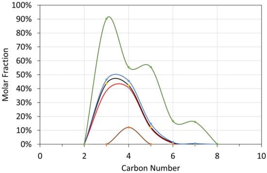
Figure A1.
Molar Gas Composition Probability Distribution as a function of carbon number: T ≤ 298 K; brown line = minimum value (0%); red line = first quartile value (25%); black line = median value (50%); blue line = third quartile value (75%); green line = maximum value (100%). A value of 75% means that there is a 75% probability, that the molar fraction of the specific carbon species, will have a lower value.
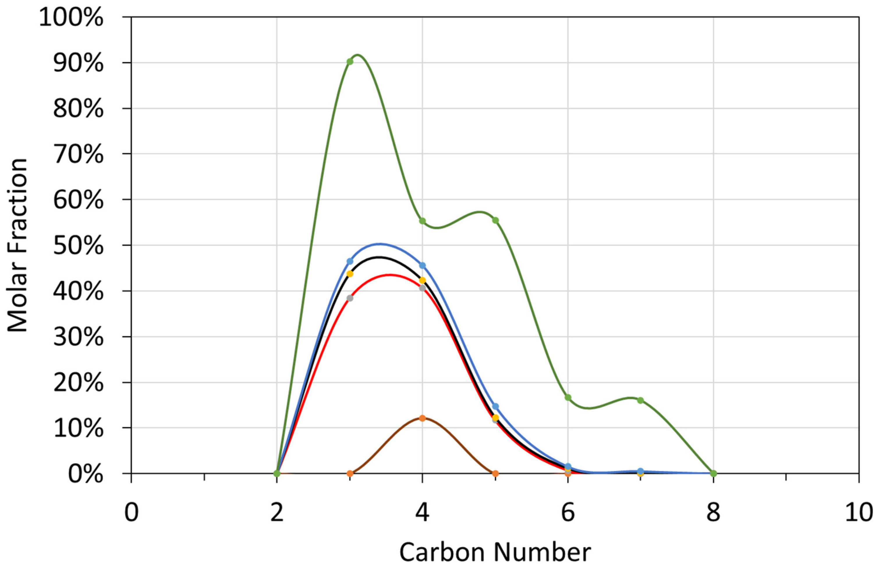
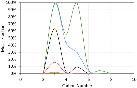
Figure A2.
Molar Gas Composition Probability Distribution as a function of carbon number T = 348 K;. brown line = minimum value (0%); red line = first quartile value (25%); black line = median value (50%); blue line = third quartile value (75%); green line = maximum value (100%).
Figure A2.
Molar Gas Composition Probability Distribution as a function of carbon number T = 348 K;. brown line = minimum value (0%); red line = first quartile value (25%); black line = median value (50%); blue line = third quartile value (75%); green line = maximum value (100%).
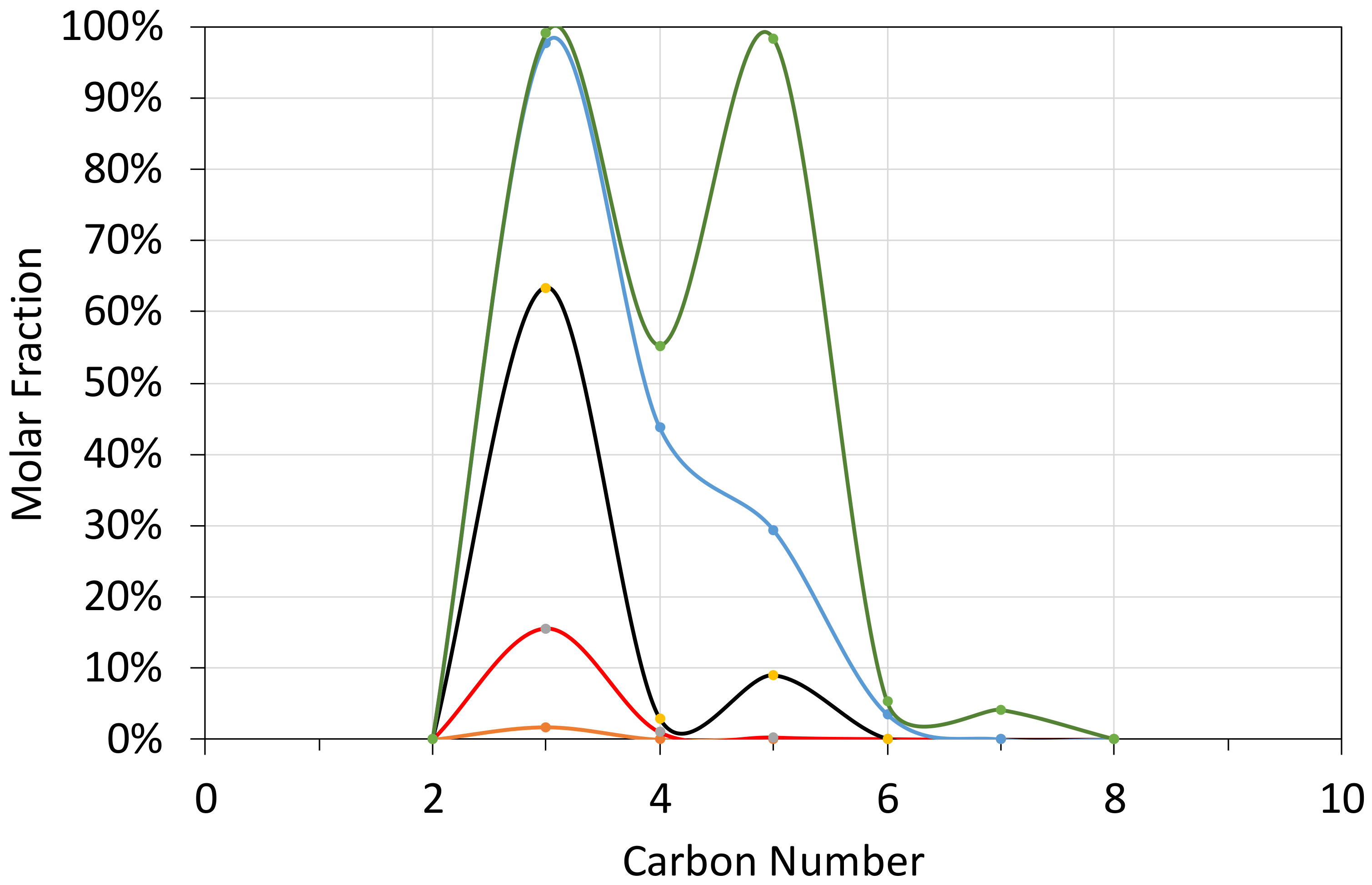
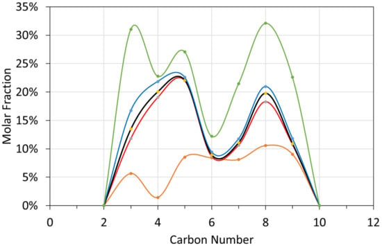
Figure A3.
Molar liquid composition probability distribution vs. carbon number: T ≤ 298 K; brown = minimum; red = first quartile; black = median; blue = third quartile; green = maximum. brown line = minimum value (0%); red line = first quartile value (25%); black line = median value (50%); blue line = third quartile value (75%); green line = maximum value (100%).
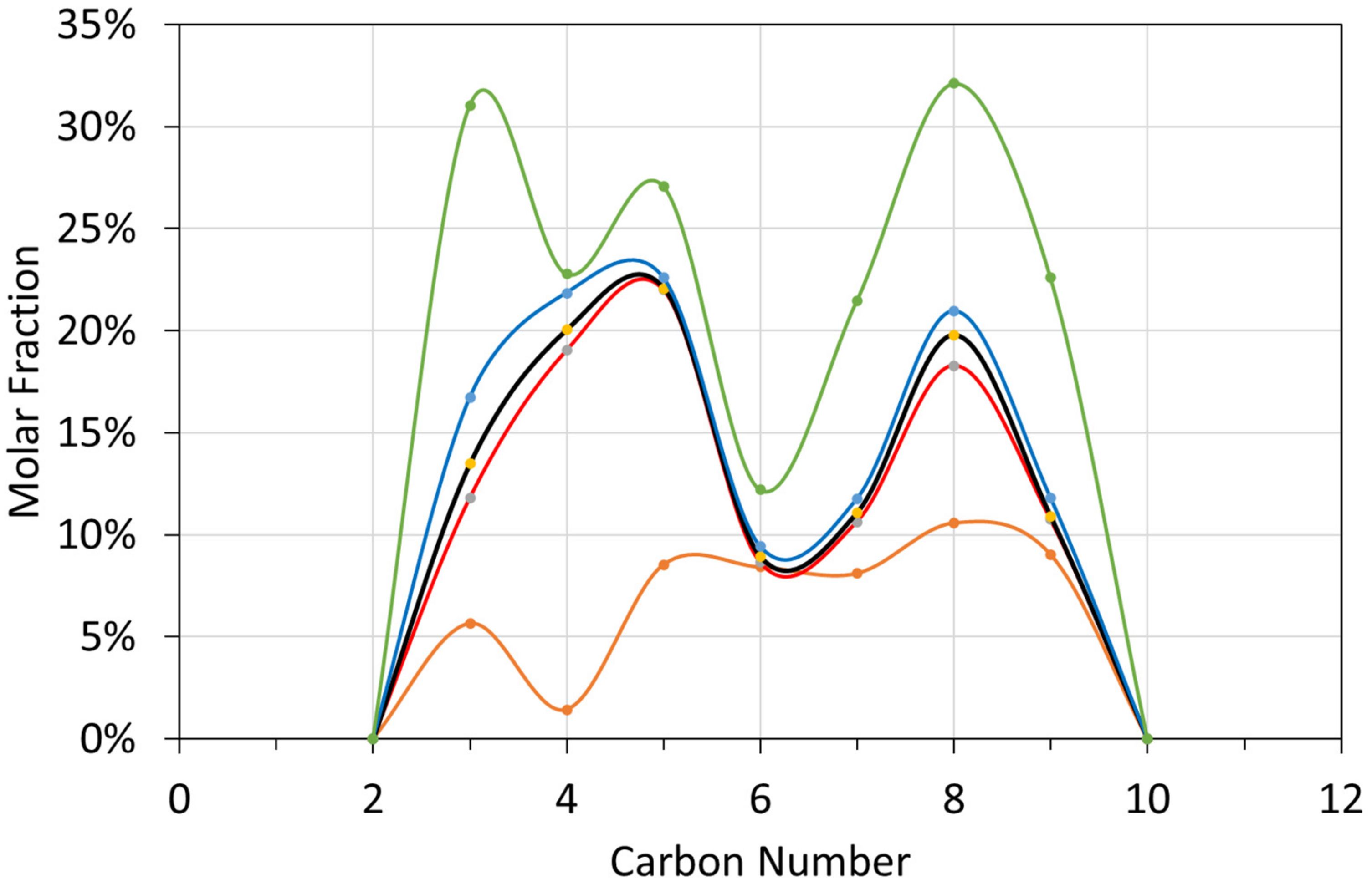
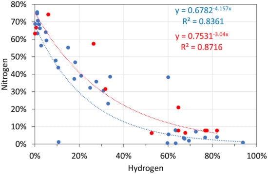
Figure A4.
Molar gas analyses: hydrogen vs. nitrogen. Blue circles: T ≤ 298 K; red circles: T = 348 K.
Figure A4.
Molar gas analyses: hydrogen vs. nitrogen. Blue circles: T ≤ 298 K; red circles: T = 348 K.
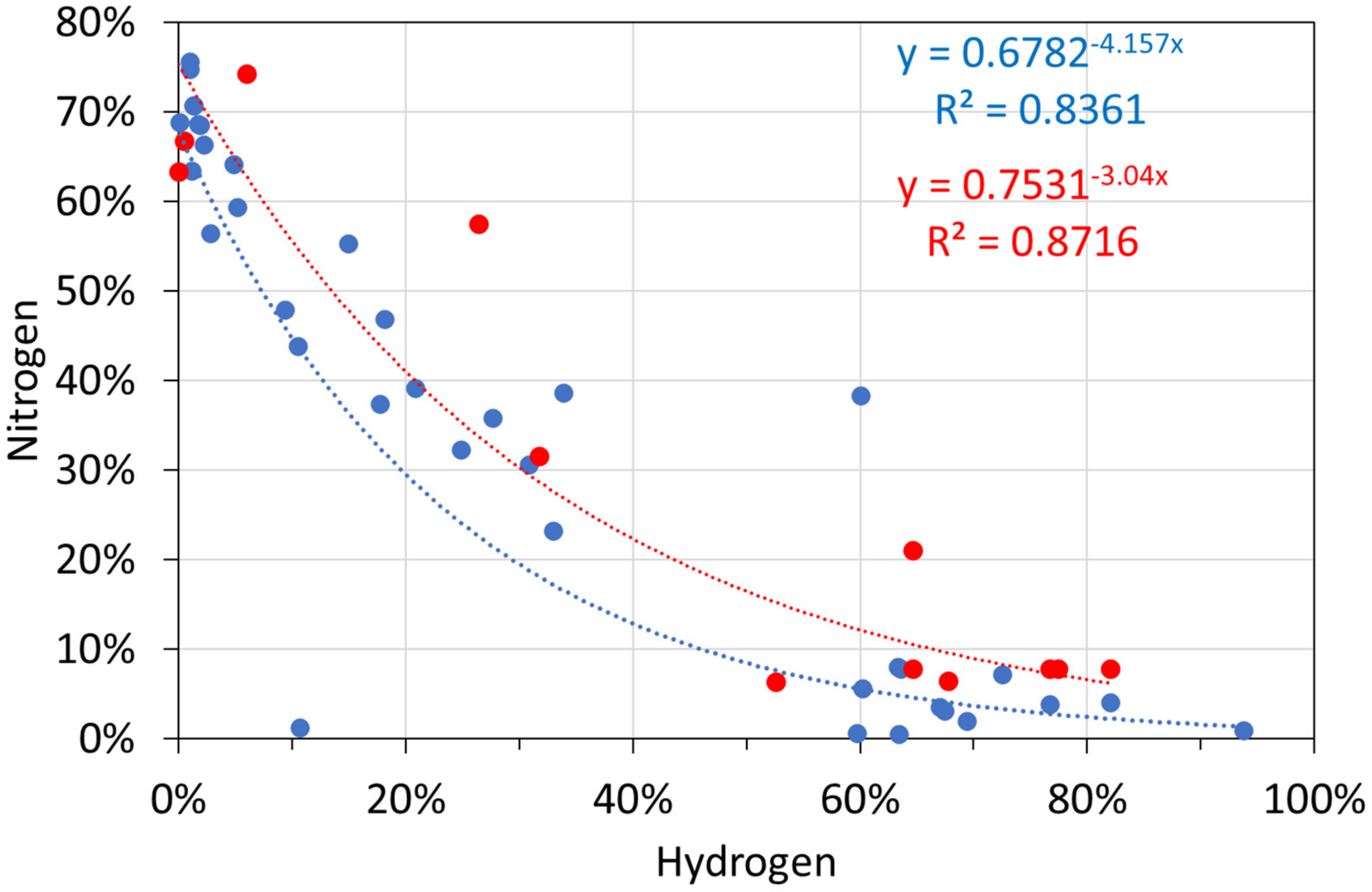

Figure A5.
Molar gas analyses: hydrogen vs. alkanes. Blue circles: T ≤ 298 K; red circles: T = 348 K.
Figure A5.
Molar gas analyses: hydrogen vs. alkanes. Blue circles: T ≤ 298 K; red circles: T = 348 K.
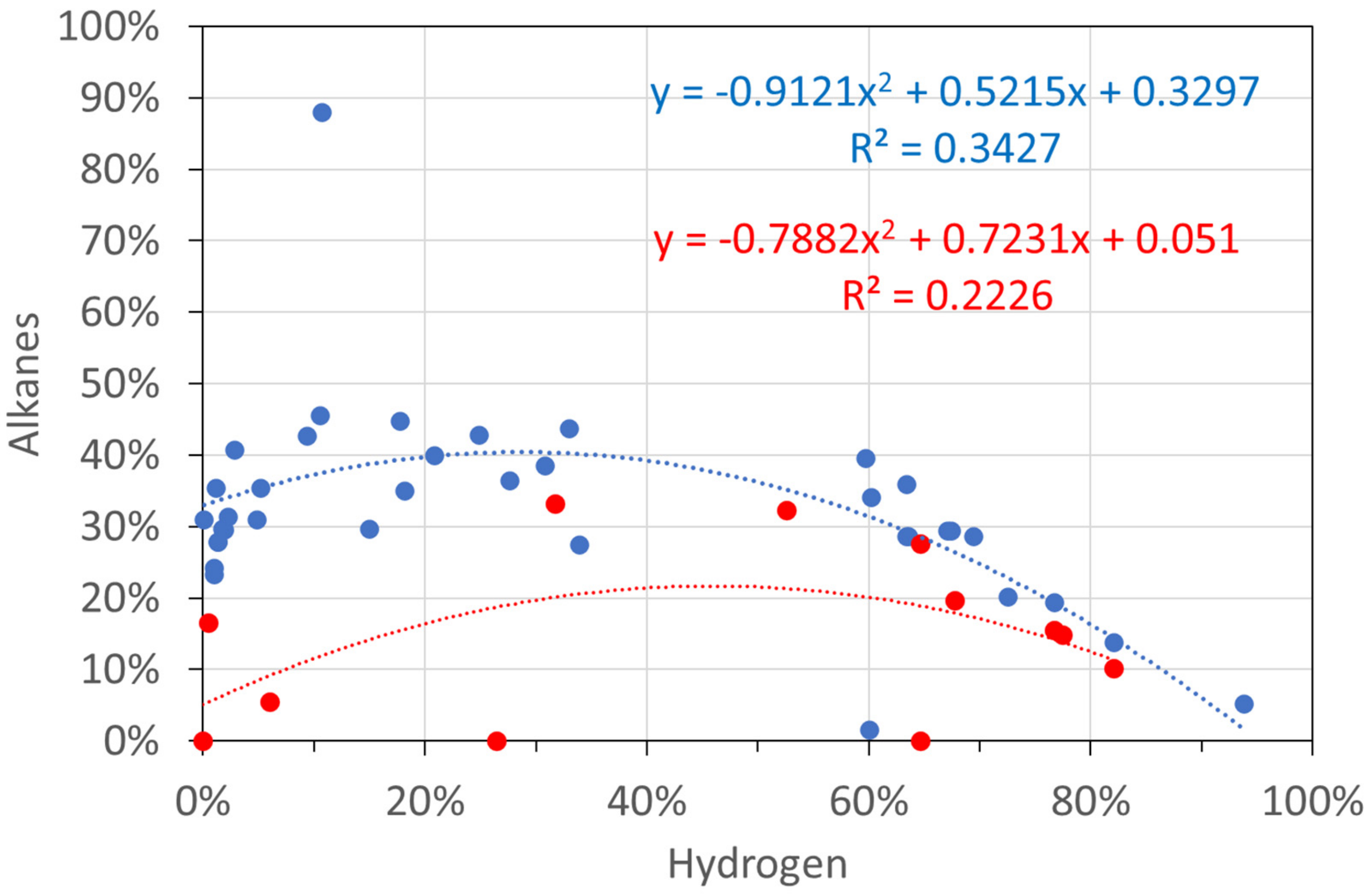

Figure A6.
Molar alkane gas analyses: propene vs. propyne. Blue circles: T ≤ 298 K; red circles: T = 348 K.
Figure A6.
Molar alkane gas analyses: propene vs. propyne. Blue circles: T ≤ 298 K; red circles: T = 348 K.
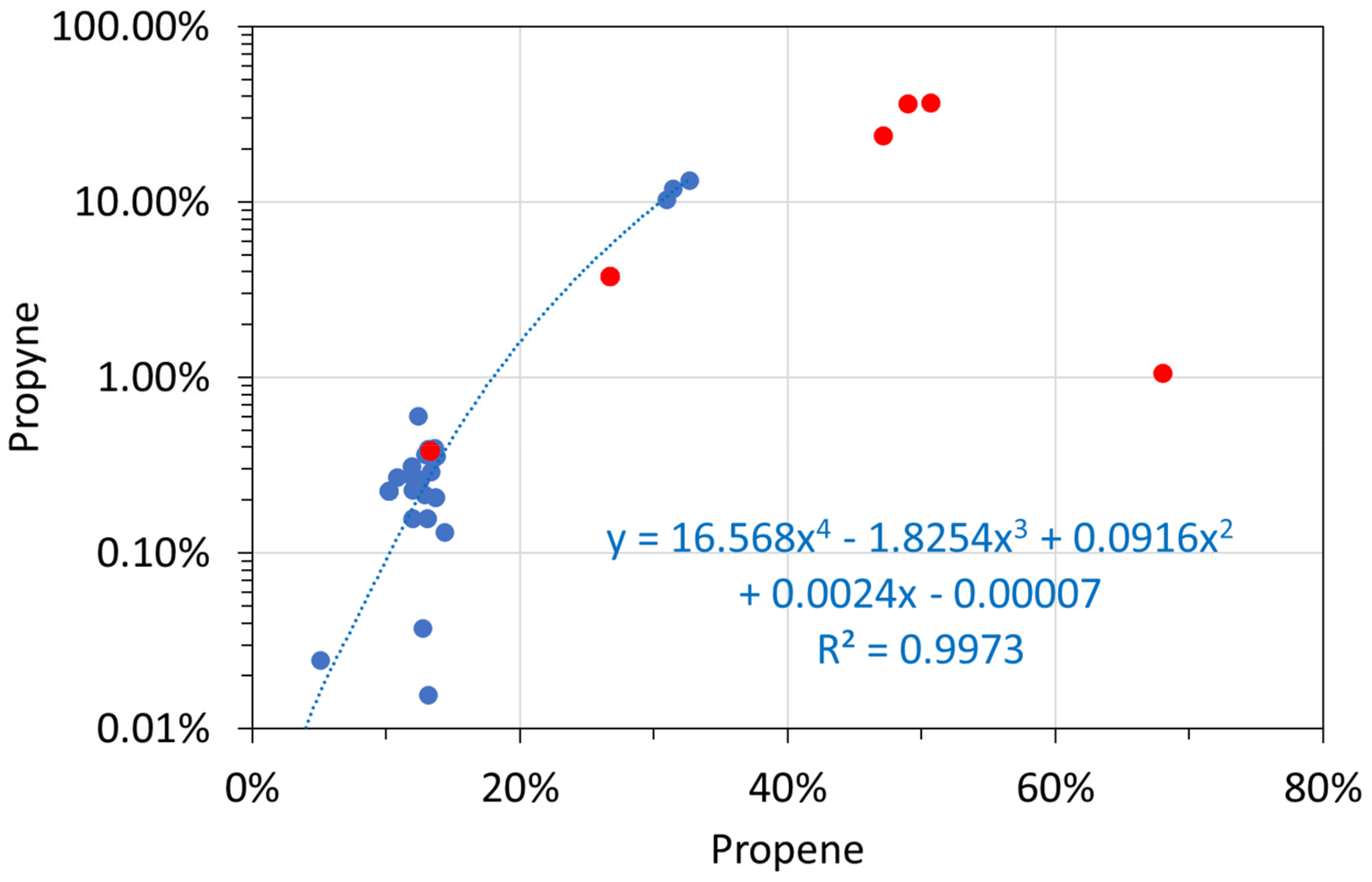
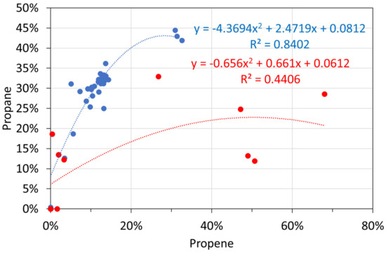
Figure A7.
Molar alkane gas analyses: propene vs. propane. Blue circles: T ≤ 298 K; red circles: T = 348 K.
Figure A7.
Molar alkane gas analyses: propene vs. propane. Blue circles: T ≤ 298 K; red circles: T = 348 K.
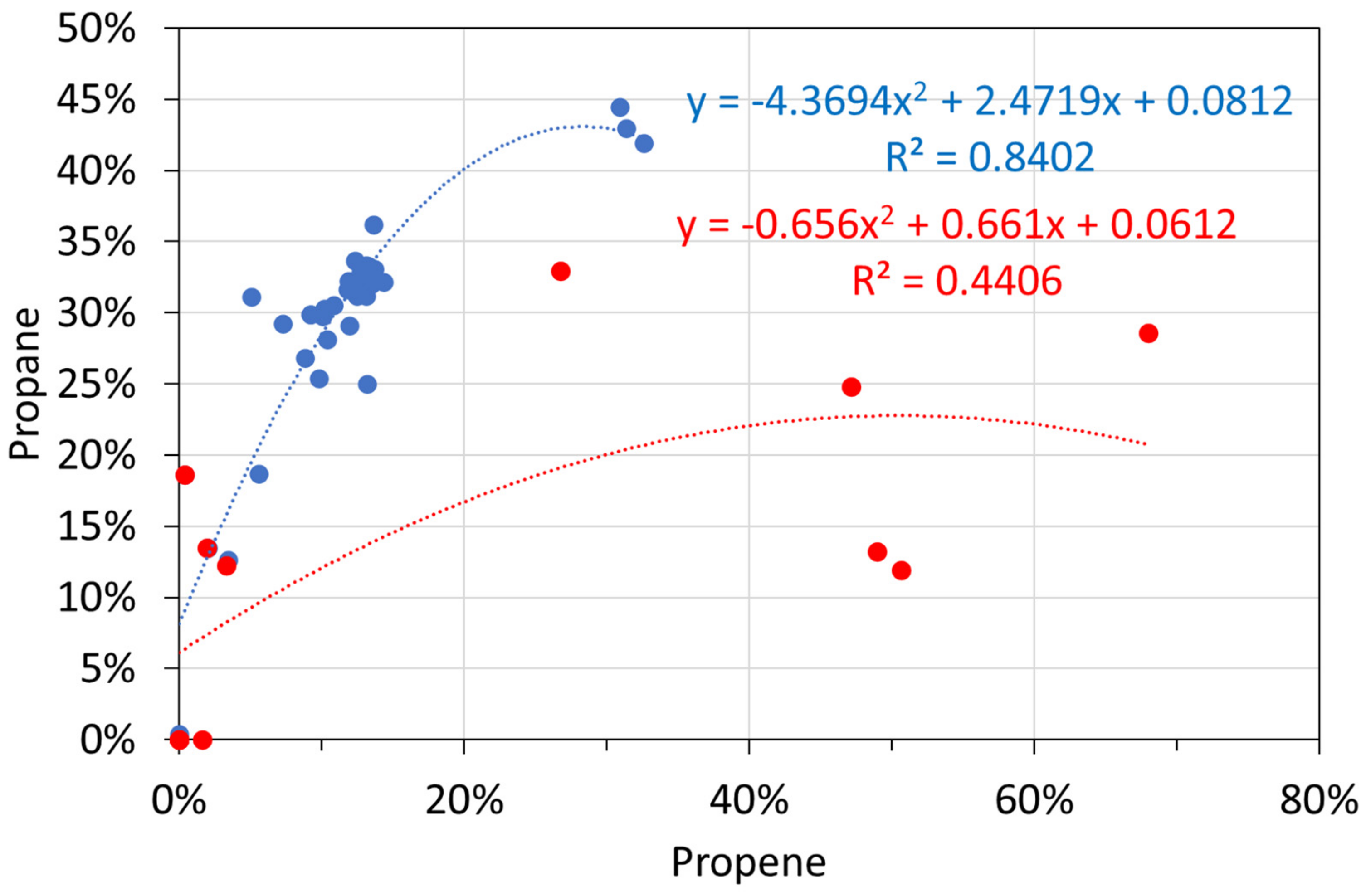
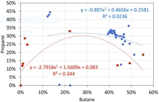
Figure A8.
Molar alkane gas analyses: butane vs. propane. Blue circles: T ≤ 298 K; red circles: T = 348 K.
Figure A8.
Molar alkane gas analyses: butane vs. propane. Blue circles: T ≤ 298 K; red circles: T = 348 K.

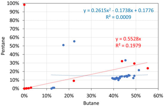
Figure A9.
Molar alkane gas analyses: butane vs. pentane. Blue circles: T ≤ 298 K; red circles: T = 348 K.
Figure A9.
Molar alkane gas analyses: butane vs. pentane. Blue circles: T ≤ 298 K; red circles: T = 348 K.
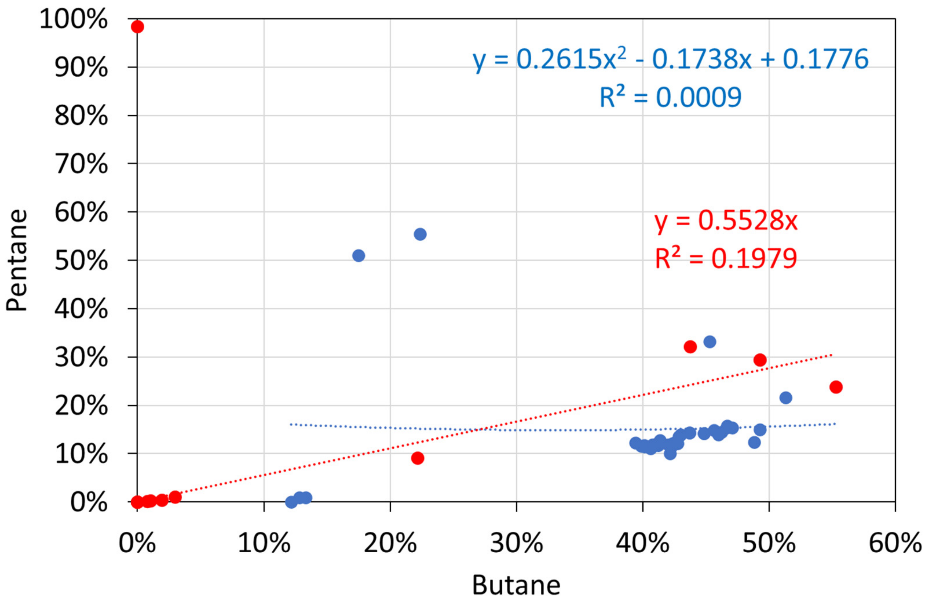
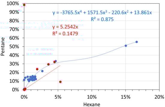
Figure A10.
Molar alkane gas analyses: hexane vs. pentane. Blue circles: T ≤ 298 K; red circles: T = 348 K.
Figure A10.
Molar alkane gas analyses: hexane vs. pentane. Blue circles: T ≤ 298 K; red circles: T = 348 K.
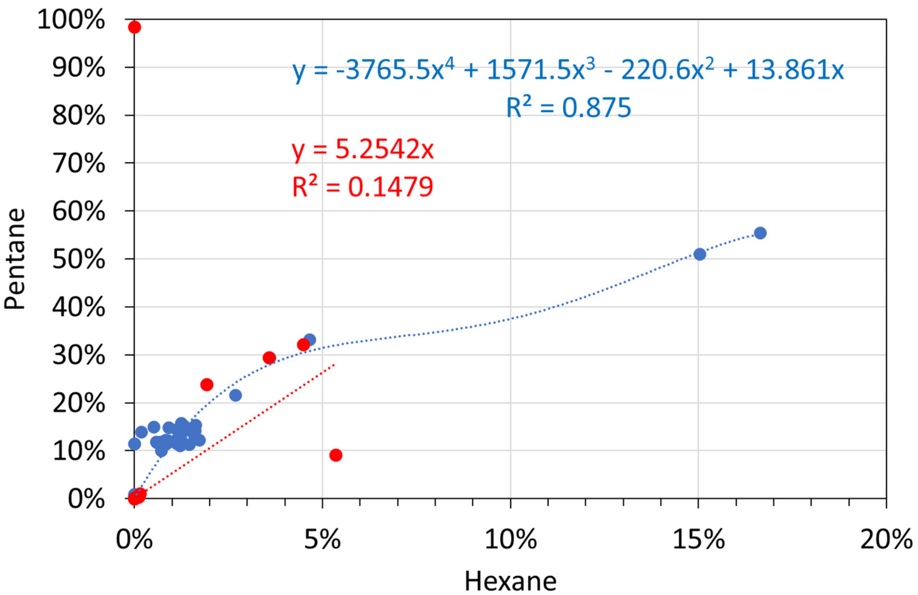
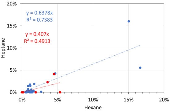
Figure A11.
Molar alkane gas analyses: hexane vs. heptane. Blue circles: T ≤ 298 K; red circles: T = 348 K.
Figure A11.
Molar alkane gas analyses: hexane vs. heptane. Blue circles: T ≤ 298 K; red circles: T = 348 K.
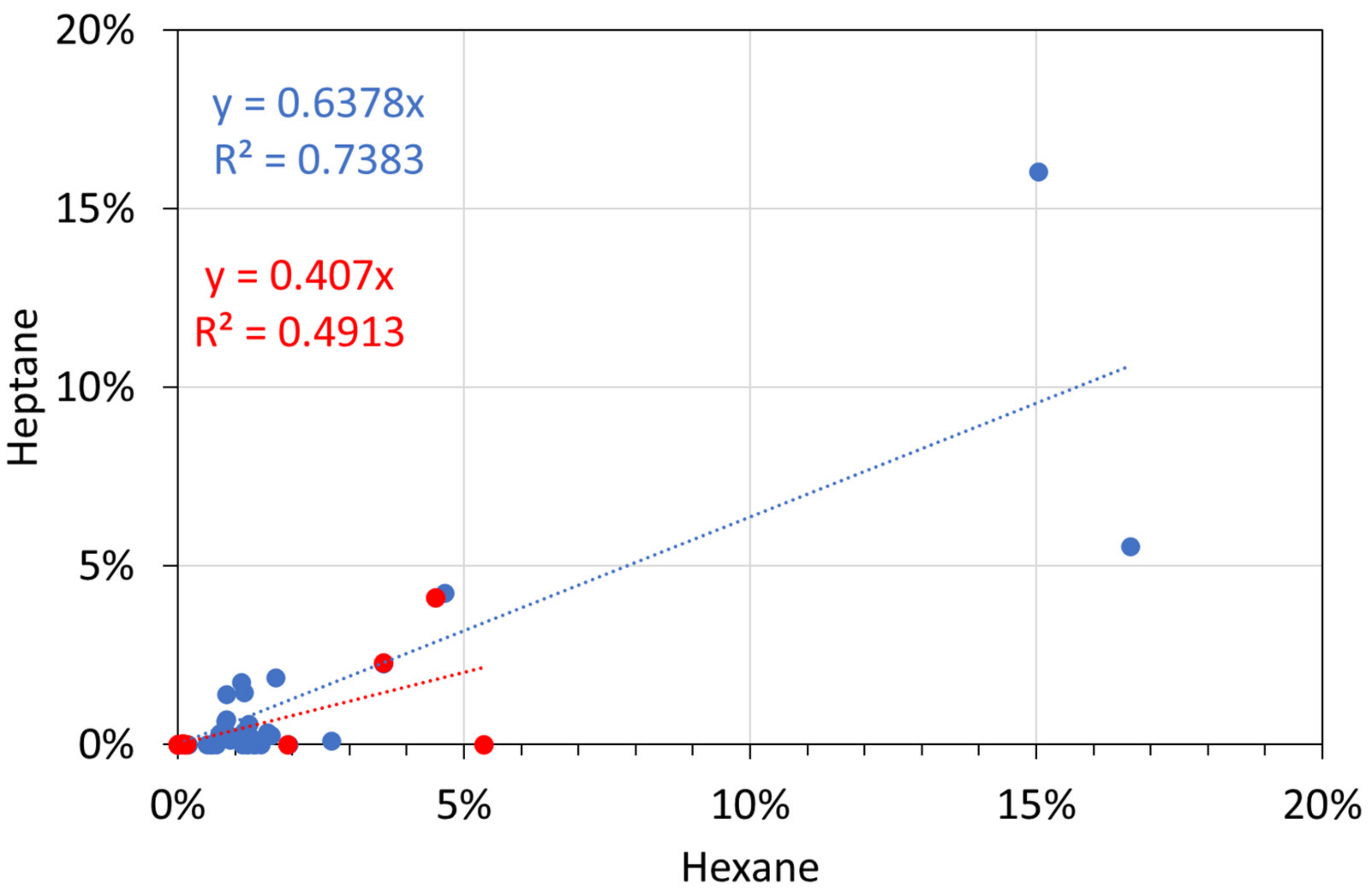
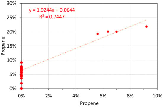
Figure A12.
Molar alkane oil analyses: propene vs. propane.
Figure A12.
Molar alkane oil analyses: propene vs. propane.
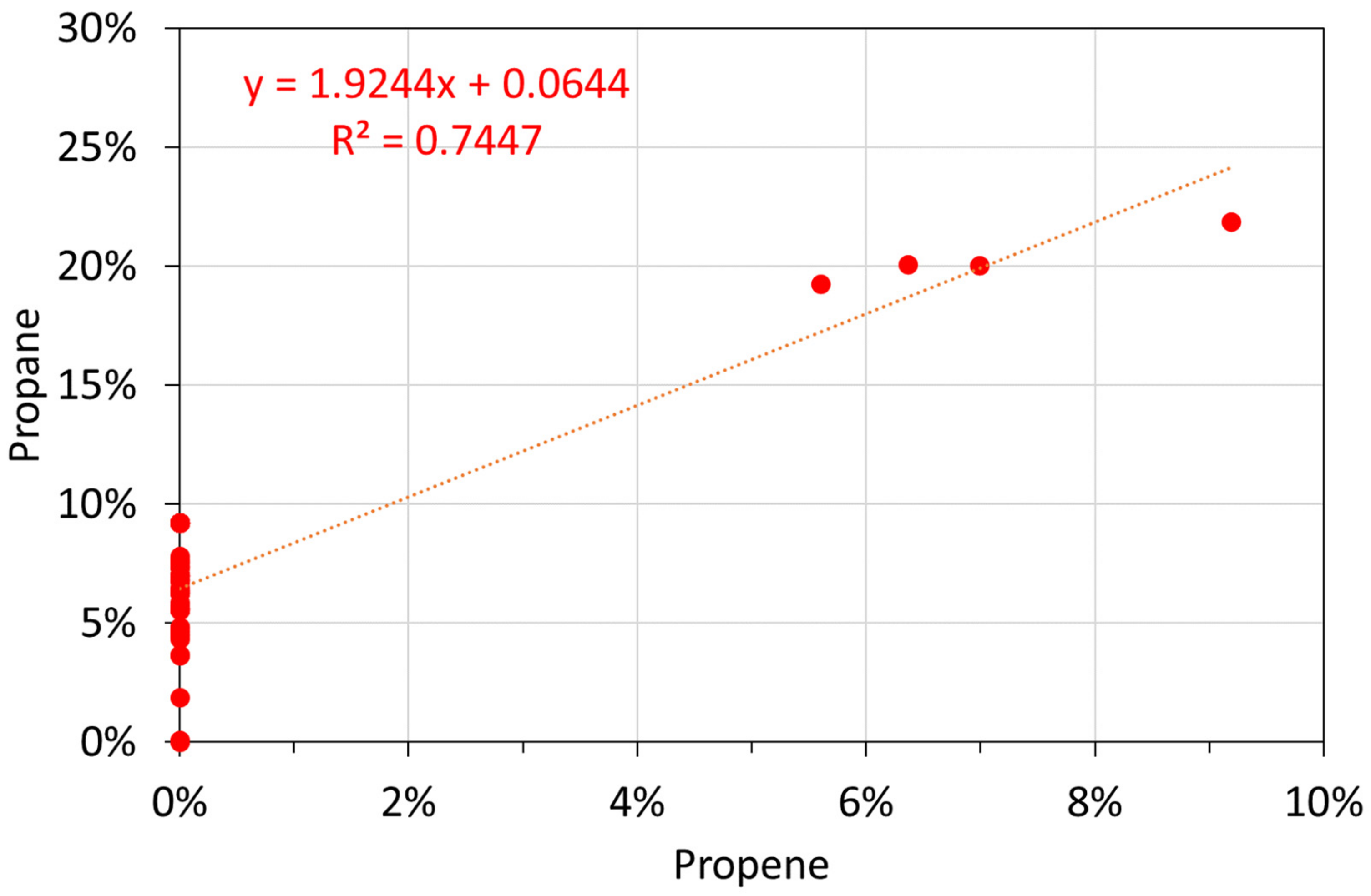

Figure A13.
Molar Alkane oil analyses: butane vs. propane.
Figure A13.
Molar Alkane oil analyses: butane vs. propane.
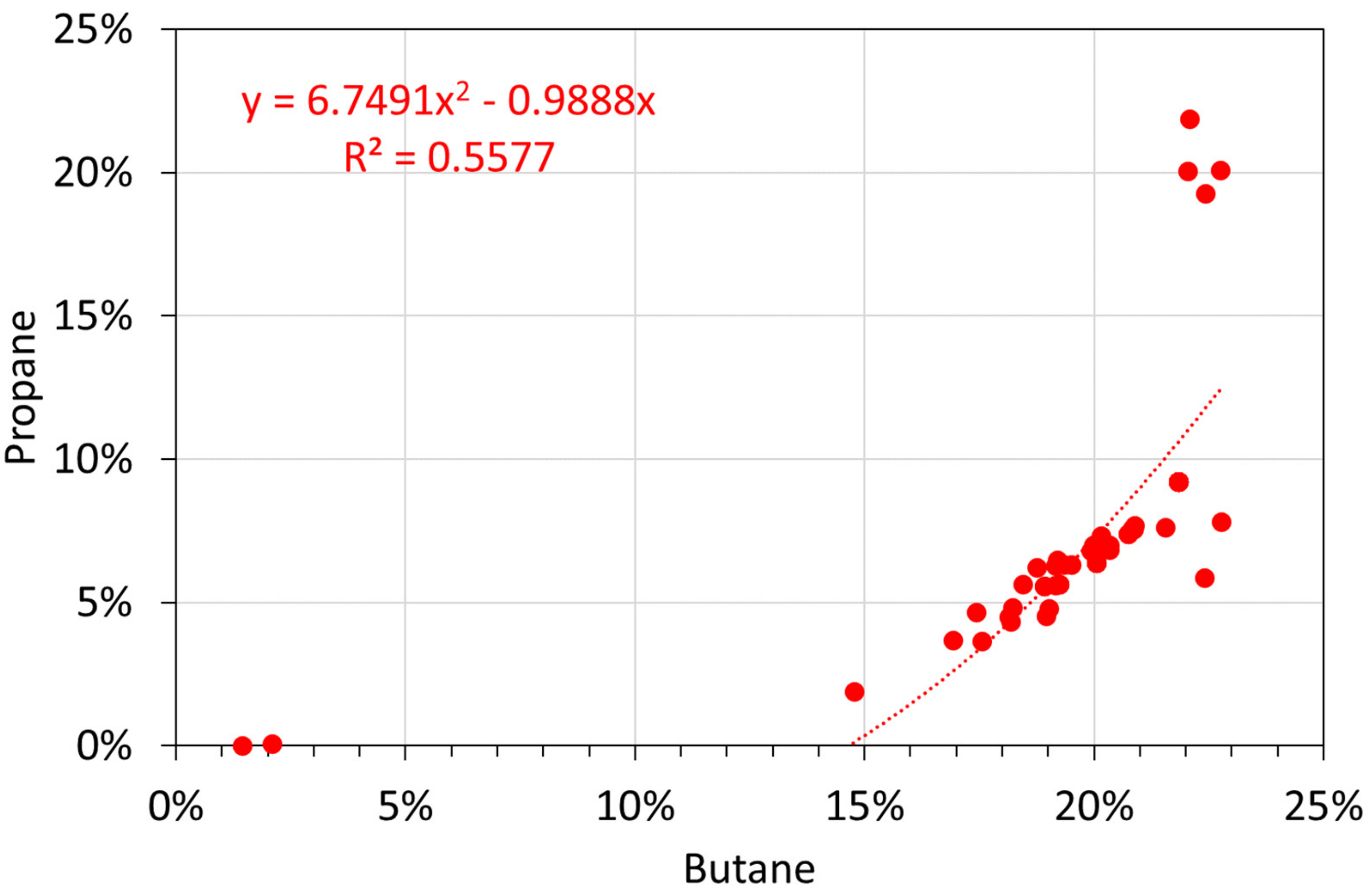
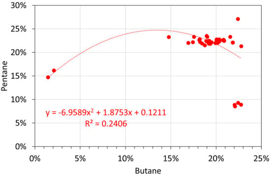
Figure A14.
Molar alkane oil analyses: butane vs. pentane.
Figure A14.
Molar alkane oil analyses: butane vs. pentane.

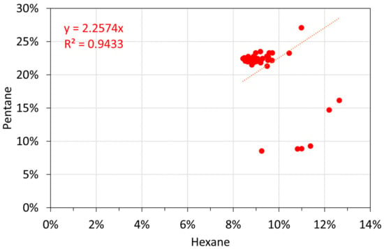
Figure A15.
Molar alkane oil analyses: hexane vs. pentane.
Figure A15.
Molar alkane oil analyses: hexane vs. pentane.
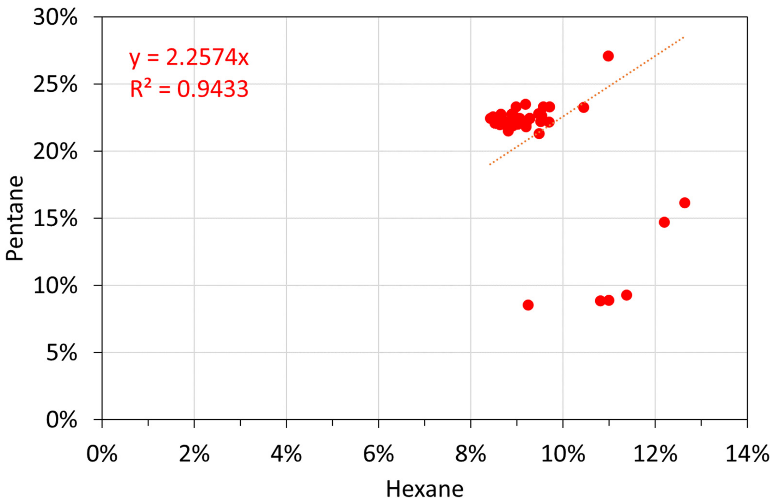
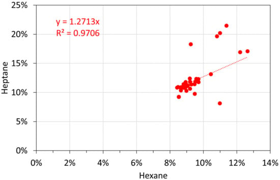
Figure A16.
Molar alkane oil analyses: hexane vs. heptane.
Figure A16.
Molar alkane oil analyses: hexane vs. heptane.

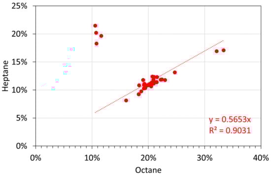
Figure A17.
Molar alkane oil analyses: octane vs. heptane.
Figure A17.
Molar alkane oil analyses: octane vs. heptane.
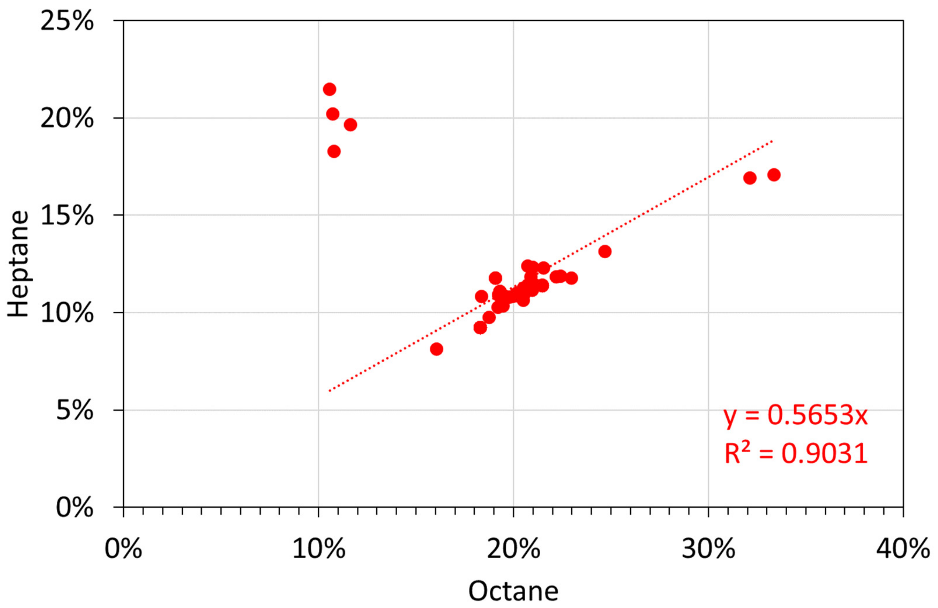
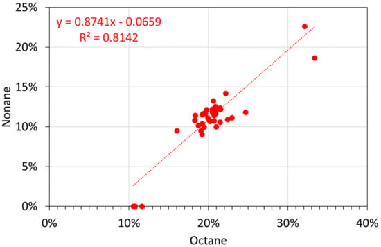
Figure A18.
Molar alkane oil analyses: octane vs. nonane.
Figure A18.
Molar alkane oil analyses: octane vs. nonane.

References
- Devonshire, E. The purification of water by means of metallic iron. J. Franklin Inst. 1890, 129, 449–461. [Google Scholar] [CrossRef]
- Antia, D.D.J. Water Treatment and Desalination Using the Eco-materials n-Fe0 (ZVI), n-Fe3O4, n-FexOyHz[mH2O], and n-Fex[Cation]nOyHz[Anion]m [rH2O]. In Handbook of Nanomaterials and Nanocomposites for Energy and Environmental Applications, 1st ed.; Kharissova, O.V., Torres-Martínez, L.M., Kharisov, B.I., Eds.; Springer: Berlin/Heidelberg, Germany, 2021; Chapter 66; pp. 3159–3242. [Google Scholar] [CrossRef]
- Noubactep, C. Metallic Iron for Water Treatment: Lost Science in the West. Bioenergetics 2017, 6, 1000149. [Google Scholar] [CrossRef] [Green Version]
- Xiao, M.; Hu, R.; Ndé-Tchoupé, A.I.; Gwenzi, W.; Noubactep, C. Metallic Iron for Water Remediation: Plenty of Room for Collaboration and Convergence to Advance the Science. Water 2022, 14, 1492. [Google Scholar] [CrossRef]
- Ali, J.; Jain, C.K. Groundwater contamination and health hazards by some of the most commonly used pesticides. Curr. Sci. 1998, 75, 1011–1014. [Google Scholar]
- Ali, A.; Burakov, A.E.; Melezhik, A.V.; Babkin, A.V.; Burkova, I.V.; Neskomornava, E.A.; Galunin, E.V.; Tkachev, A.G.; Kuznetsov, D.V. Removal of Copper(II) and Zinc(II) Ions in Water on a Newly Synthesized Polyhydroquinone/Graphene Nanocomposite Material: Kinetics, Thermodynamics and Mechanism. ChemistrySelect 2019, 4, 12708–12718. [Google Scholar] [CrossRef]
- Antia, D.D.J. Chapter 8: Direct synthesis of air-stable metal complexes for desalination (and water treatment). In Direct Synthesis of Metal Complexes, 1st ed.; Kharisov, B.I., Ed.; Elsevier: Amsterdam, The Netherlands, 2018; pp. 341–367. [Google Scholar]
- Basheer, A. Advances in the smart materials applications in the aerospace industries. Aircr. Eng. Aerosp. Technol. 2020, 92, 1027–1035. [Google Scholar] [CrossRef]
- Ali, I.; Alharbi, O.M.L.; AlOlthman, Z.A.; Alwarthan, A.; Al-Mohaimeed, A.M. Preparation of a carboxymethylcellulose-iron composite for uptake of atorvastatin in water. Int. J. Biol. Macromol. 2019, 132, 244–253. [Google Scholar] [CrossRef]
- Hu, R.; Ndé-Tchoupé, A.I.; Cao, V.; Gwenzi, W.; Noubactep, C. Metallic iron for environmental remediation: The fallacy of the electron efficiency concept. Front. Environ. Chem. 2021, 2, 677813. [Google Scholar] [CrossRef]
- Hu, R.; Noubactep, C. Redirecting research on Fe0 for environmental remediation: The search for synergy. Int. J. Environ. Res. Public Health 2019, 16, 4465. [Google Scholar] [CrossRef] [Green Version]
- Noubactep, C. The operating mode of Fe0/H2O systems: Hidden truth or repeated nonsense? Fresenius Environ. Bull. 2019, 28, 8328–8330. [Google Scholar]
- Hu, R.; Gwenzi, G.; Sipowo-Tala, V.R.; Noubactep, C. Water treatment using metallic iron: A tutorial review. Processes 2019, 7, 622. [Google Scholar] [CrossRef] [Green Version]
- Pourbaix, M. Atlas of Electrochemical Equilibria in Aqueous Solutions; NACE International: Houston, TX, USA, 1974; p. 644. [Google Scholar]
- Hardy, L.I.; Gillham, R.W. Formation of hydrocarbons from the reduction of aqueous CO2 by zero-valent iron. Environ. Sci. Technol. 1996, 30, 57–65. [Google Scholar] [CrossRef]
- Deng, B.; Campbell, T.J.; Burris, D.R. Hydrocarbon formation in metallic iron/water systems. Environ. Sci. Technol. 1997, 31, 1185–1190. [Google Scholar] [CrossRef]
- Cvetković, B.Z.; Rothardt, J.; Büttler, A.; Kunz, D.; Schlotterbeck, G.; Wieland, E. Formation of Low-Molecular-Weight Organic Compounds During Anoxic Corrosion of Zero-Valent Iron. Environ. Eng. Sci. 2018, 35, 447–461. [Google Scholar] [CrossRef]
- Guillemont, T.; Cvetkovic, B.Z.; Kunz, D.; Weiland, E. Processes leading to reduced and oxidised carbon compounds during corrosion of zero-valent iron in alkaline anoxic conditions. Chemosphere 2020, 250, 126230. [Google Scholar] [CrossRef] [PubMed]
- Guillemont, T.; Salazar, G.; Cvetkovic, B.Z.; Kunz, D.; Szidat, S.; Wieland, E. Determination of ultra-low concentrations of gaseous 14C-bearing hydrocarbons produced during corrosion of irradiated steel using accelerator mass spectrometry. Analyst 2020, 145, 7870–7883. [Google Scholar] [CrossRef]
- Fogel, S. Reactions of zero-valent iron with groundwater containing high concentrations of carbon tetrachloride. In Proceedings of the Fourth International Conference on Remediation of Chlorinated and Recalcitrant Compounds, Monterey, CA, USA, 24–27 May 2004; Gavaskar, A.R., Chen, A.S.C., Eds.; Battelle Press: Columbus, OH, USA, 2004. ISBN 1-57477-145-0. [Google Scholar]
- Zhang, Z.-Y.; Lu, M.; Zhang, Z.-Z.; Xiao, M.; Zhang, M. Dechlorination of short chain chlorinated paraffins by nanoscale zero-valent iron. J. Hazard. Mater. 2012, 243, 105–111. [Google Scholar] [CrossRef]
- Lin, K.-S.; Dehvari, K.; Hsien, M.-J.; Hsu, P.-J.; Kuo, H. Degradation of TNT, RDX, and HMX Explosive Wastewaters Using Zero-Valent Iron Nanoparticles. Propellants Explos. Pyrotech. 2013, 38, 786–790. [Google Scholar] [CrossRef]
- Hara, J.; Ito, H.; Suto, K.; Inoue, C.; Chida, T. Kinetics of trichloroethene dechlorination with iron powder. Water Res. 2005, 39, 1165–1173. [Google Scholar] [CrossRef]
- Pang, H.; Liu, L.; Bai, Z.; Chen, R.; Tang, C.; Cai, Y.; Yu, S.; Hu, B.; Wang, X. Fabrication of sulfide nanoscale zero-valent iron and heterogeneous Fenton-like degradation of 2,4-Dichlorophenol. Sep. Purif. Technol. 2022, 285, 120408. [Google Scholar] [CrossRef]
- Ghauch, A.; Gallet, C.; Charef, A.; Rima, J.; Martin-Bouyer, M. Reductive degradation of carbaryl in water by Zero-valent iron. Chemosphere 2001, 42, 419–424. [Google Scholar] [CrossRef]
- Sawama, Y.; Ban, K.; Akusu-Suyama, K.; Nakata, H.; Mori, M.; Yamada, T.; Kawajiri, T.; Yasukawa, N.; Park, K.; Monguchi, Y. Birch-Type Reduction of Arenes in 2-Propanol Catalysed by Zero Valent Iron and Platinum on Carbon. ACS Omega 2019, 4, 11522–11531. [Google Scholar] [CrossRef] [PubMed]
- Patil, R.D.; Sasson, Y. Generation of Hydrogen from Zero-Valent Iron and Water: Catalytic Transfer Hydrogenation of Olefins in Presence of Pd/C. Asian J. Org. Chem. 2015, 4, 1258–1261. [Google Scholar] [CrossRef]
- Shukla, P.R.; Skea, J.; Slade, R.; Al Khourdajie, A.; van Diemen, R.; McCollum, D.; Pathak, M.; Some, S.; Vyas, P.; Fradera, R.; et al. (Eds.) IPCC Climate Change 2022: Mitigation of Climate Change. In Contribution of Working Group III to the Sixth Assessment Report of the Intergovernmental Panel on Climate Change; Cambridge University Press: Cambridge, UK; New York, NY, USA, 2022. [Google Scholar] [CrossRef]
- Shukla, P.R.; Skea, J.; Slade, R.; Al Khourdajie, A.; van Diemen, R.; McCollum, D.; Pathak, M.; Some, S.; Vyas, P.; Fradera, R.; et al. (Eds.) IPCC Summary for Policymakers. In Climate Change 2022: Mitigation of Climate Change. Contribution of Working Group III to the Sixth Assessment Report of the Intergovernmental Panel on Climate Change; Cambridge University Press: Cambridge, UK; New York, NY, USA, 2022. [Google Scholar] [CrossRef]
- Antia, D.D.J. Hydrocarbon formation in immature sediments. Adv. Pet. Explor. Dev. 2011, 1, 1–13. [Google Scholar] [CrossRef]
- Ebbing, D.D.; Gammon, S.D. General Chemistry; Houghton Mifflin Company: New York, NY, USA, 2005; ISBN 0-618-399410. [Google Scholar]
- British Standards Institute. Quality management systems, BSI Handbook 25. In Statistical Interpretation of Data; British Standards Institute: London, UK, 1985; p. 318. ISBN 0580150712, 9780580150715. [Google Scholar]
- Mulder, M. Basic Principles of Membrane Technology, 2nd ed.; Kluwer Academic Publishers: Dordrecht, The Netherlands, 1996; p. 564. ISBN 0-7923-427-X. [Google Scholar]
- Weststrate, C.J.; van Helden, P.; Niemantsverdriet, J.W. Reflections on the Fischer-Tropsch synthesis: Mechanistic issues from a surface science perspective. Catal. Today 2016, 275, 100–110. [Google Scholar] [CrossRef]
- Antia, D.D.J. Oil polymerisation and fluid expulsion from low temperature, low maturity, over pressured sediments. J. Petrol. Geol. 2008, 31, 263–282. [Google Scholar] [CrossRef]
- Davis, B.H. Fischer–Tropsch Synthesis: Reaction mechanisms for iron catalysts. Catal. Today 2009, 141, 25–33. [Google Scholar] [CrossRef]
- Fillpa, L.; Zamostny, P.; Rauch, R. Mathematical model of Fischer-Tropsch synthesis using variable alpha-parameter to predict product distribution. Fuel 2018, 243, 603–609. [Google Scholar] [CrossRef]
- Kruit, K.D.; Vervloet, D.; Kapteijn, F.; van Ommen, J.R. Selectivity of the Fischer–Tropsch process: Deviations from single alpha product distribution explained by gradients in process conditions. Catal. Sci. Technol. 2013, 3, 2210–2213. [Google Scholar] [CrossRef] [Green Version]
- Chen, K.-F.; Li, S.; Zhang, W.-X. Renewable hydrogen generation by bimetallic zero valent iron nanoparticles. Chem. Eng. J. 2011, 170, 562–567. [Google Scholar] [CrossRef]
- Reardon, E.J. Capture and storage of hydrogen gas by zero-valent iron. J. Contam. Hydrol. 2015, 157, 117–124. [Google Scholar] [CrossRef] [PubMed]
- Fischer, F.; Tropsch, H. Composition of products obtained by the petroleum synthesis. Brennst Chem. 1928, 9, 21–24. [Google Scholar]
- Storch, H.H.; Golumbic, N.; Anderson, R.B. The Fischer-Tropsch and Related Synthesis; John Wiley & Sons Inc.: New York, NY, USA, 1951; p. 610. [Google Scholar]
- Lide, D.R. CRC Handbook of Chemistry & Physics, 89th ed.; CRC Press: Boca Raton, FL, USA, 2008; ISBN 13-978-1-4200-6679-1. [Google Scholar]
- Ellis, H. Book of Data; Longman Group: Harlow, UK, 1984; ISBN 058035448X. [Google Scholar]

Publisher’s Note: MDPI stays neutral with regard to jurisdictional claims in published maps and institutional affiliations. |
© 2022 by the author. Licensee MDPI, Basel, Switzerland. This article is an open access article distributed under the terms and conditions of the Creative Commons Attribution (CC BY) license (https://creativecommons.org/licenses/by/4.0/).