A Moment-Based Depth-Averaged K-ε Model for Predicting the True Turbulence Intensity over Bedforms

Abstract

Turbulence models are critical for depth-averaged flow models in at least two ways: (i) as closures for momentum equations and (ii) as indicators of the spatial variability in the turbulence intensity field, which is crucial for sediment transport and bedform evolutions. This paper introduces a novel moment-based depth-averaged k-ε turbulence (MDAKE) model that could be considered as a revised version for the standard k-ε Rastogi–Rodi (SDAKE) model and can be used to estimate the true values for the depth-averaged turbulence kinetic energy in more complex and varied flow conditions with accelerating–decelerating flow fields. The study in hand shows that the SDAKE model tends to overestimate the true depth-averaged turbulent kinetic energy (${\overline{k}}_u$) by 50 to 130% in the benchmark case of uniform flow over a flatbed. Further, the SDAKE model assumes that the bed shear velocity is an appropriate scale for the generation terms of both turbulent kinetic energy and dissipation. When bed topographic features vary, a shear flow zone is formed and the assumption is invalid. Since most of the turbulence is generated by shear flow zones away from the bed, the SDAKE model’s estimates for the depth-averaged turbulent kinetic energy field are out of phase with measurements for the flow over a train of bedforms. Therefore, a newly developed depth-averaged KE model based on the moment concept (MDAKE) is presented here. The model replaces bed shear velocity with the integral moment velocity scale ($u_1$). The calibrated MDAKE model is used to predict turbulent kinetic energy over a train of bedforms. The results of the MDAKE model are in phase and generally in reasonable agreement with the measurements.

1. Introduction

Depth-averaged flow models are considered one of the basic simulation tools commonly used in many river engineering applications [1,2]. On the one hand, depth-averaged models are characterized by their simplicity and their relatively limited input data and computer resource requirements. On the other hand, the models overlook the vertical velocity details due to the depth-averaging approximation and, thus, these models only use one velocity scale, the depth-averaged velocity, in each flow direction. As a result, depth-averaged models were not able to accurately map the spatial variation in the flow and turbulence structure over a varying bed terrain, such as the case of shallow water flowing over a train of bedforms and dunes [3,4].

To extend the capabilities of depth-averaged models, the moment-of-momentum concept was introduced [5] and a new generation of depth-averaged models, called vertically averaged and moment models (VAM), was developed. In these VAM models, the degrees of freedom for the velocity profile are increased from a typically constant mean value (in the conventional depth-averaged models) to a linear or parabolic distribution (in the VAM models). In addition, the hydrostatic assumption could be released and the non-hydrostatic effect could be considered [5].

Both depth-averaged models and VAM flow models require the use of relevant turbulence models, mainly to work as closure equations for the mathematical differential terms resulting from the time averaging of the Navier Stocks equations and to capture the dominating length and velocity scales in the turbulence/eddy structure of the flow field [6,7,8,9,10,11,12]. The two-transport equations model (Rastogi and Rodi’s k-ε model) is the standard turbulence closure model that was introduced early in 1978 for depth-averaged models [13]. Over the last four decades, the standard k-ε model and its revised versions (k-w and others) have been widely used with the depth-averaged models to investigate a broad range of applications, including open stream flow, coastal engineering, thermal diffusion and sediment transport [13,14,15,16,17].

In the past, it was believed that bed-load sediment transport depends mainly on bed shear stress. Recent studies and experimental investigations pointed out that for non-uniform boundary layer cases, the entrainment of sediment is not a unique function of the local bed shear stress [18,19,20]. Flows with high turbulence intensities are capable of moving more total sediment than those with low ones for the same given bed shear stress. Mclean and his research group indirectly measured the local bed sediment transport rate of an erodible sand form by measuring the bed levels of the bedform via two acoustic-profiler runs [20]. They noticed that the measured transport just downstream from the point of reattachment, where the shear stress is close to zero, is significantly greater than the prediction using a bed shear-stress-based formula.

The turbulence models could be also used to describe the spatial variability in the turbulence intensity field. This description might be essential for some applications where the turbulence plays an important role, such as: the transport of sediment, the evolution of bedforms and mixing of tracers and water quality investigations.

In the literature on sediment transport, bedload is the subject of various research schools, with diverse approaches used to assess it. The bed shear-stress-based method is the first and most famous approach that relies on the local bed shear stress as an independent parameter for estimating the bedload transport rate. A second approach is the individual soil particle-tracking-based or grain-level method. This method follows a Lagrangian approach in examining the hydrodynamic forces acting on individual soil particles to identify whether the driving forces are sufficient to overcome the other weight and resisting forces, such that the particles move or rest. The work of Lee et al. [21] is a good example of this approach. The third approach is the “turbulence-induced bedload” approach. In this method, researchers are attempting to estimate bedload transport using either turbulent kinetic energy (k) or other turbulence statistics. Examples of the research work for this last method are mentioned below.

Turbulence plays an important role, not only for suspended load but also for bedload transport as well. Bedload transport generally comprises a number of transportation modes, which include: sliding, rolling and saltating modes [22]. The saltation of bed particles is primarily controlled by hydrodynamic drag (FD) and lift (FL) forces. In the case of turbulent flow, the lift forces are highly influenced by the near-bed turbulence field. Consequently, turbulence could have a direct effect not only on suspended load transport but also on bedload transport as well. In 2018, Barati et al. [23] studied the saltation mode of the bedload sediment transport and they concluded that both of “the shear lift force and turbulent flow fluctuations are important factors for the saltation of both sand and gravel particles, and they cannot be ignored”. With the help of video analysis and LDV/UPV instruments, Nelson et al. in 1995 [19] and, more recently, Radice et al. in 2013 [24] and others studied the role of a near-bed turbulence structure, specifically in bedload transport using quadrant analysis techniques. These studies have shown that the local bed shear stress includes only the turbulence events that belong to quad 4 (“sweeps”) and quad 2 (“bursts or ejections”). This means that any turbulence events taking place in quads 1 and 3 (outward and inward interactions, respectively) are not presented by the local bed shear stress. In 2010, Paiement et al. [25] carried out an in-situ experiment to measure the bedload transport and turbulence statistics in one of the gravel-bed rivers in (Quebec, QC, Canada). The study documented the effect of the instantaneous fluid acceleration–deceleration and the vertical normal stress component on the bedload transport rate.

In 2018, Zgheib et al. [26] used a high-resolution direct numerical simulation (DNS) method to study the effect of the bed vortical structures on the bed formations. They mentioned that the role of the local bed vortical structures is essential during the early stages of bed formations, starting from the formation of streaks to the creation of chevron features and the formation of the incipient crestlines of ripples. Nevertheless, the effects of these bed-vortical structures become of marginal importance in the later stages when the bedforms become bigger in size and sufficiently matured. In this case, the macro-roughness of the bedform governs the flow structure and the turbulence production becomes mainly generated by shear flow zones downstream the crest of the bedform. In 2021, Guan et al. [27] used the DNS model to simulate the turbulence flow over a mobile bed. Their model was able to capture the existence of the bed-penetrating Kelvin–Helmholtz (KH) vortex packets and to study its effect on the discrepancies between the instantaneous local bedload transport and the predicted values by the Wong and Parker formula. In 2018, Yang, and Nepf [28] presented their first turbulence-based bedload transport model for bare and vegetated beds. They used the turbulent kinetic energy (k) instead of the bed shear stress as a predictor for the bedload sediment transport.

By considering the turbulence field in the sediment transport analysis, a better understanding of the actual bedload transport could be obtained, especially in cases of non-uniform boundary conditions, such as flow over a bedform. This will help in obtaining more accurate predictions for the temporal variation in bed-stream resistance in natural rivers during the different stages of the flood events.

The purpose of this study is to present a revised version of the standard 1D depth-averaged k-ε (SDAKE) model. The revised version (MDAKE) is based on the moment-of-momentum approach and it can be used to predict the variations in the depth-averaged turbulent kinetic energy field in cases of flowing water over a varying bed topography.

The study in hand has three primary objectives:

-

Investigate the typical spatial variability in the depth-averaged turbulent kinetic energy field over a train of bedforms based on experimental studies reported in the literature;

-

Assess the accuracy and limitations of the standard k-ε depth-averaged turbulence SDAKE model in reproducing the measured values of turbulent kinetic energy in both the benchmark uniform flow over a flatbed case as well as the case for flow over a train of bedforms;

-

Introduce a new k-ε turbulent (MDAKE) model that is based on the moment concept and suitable for depth-averaged VAM models and can be used to reasonably predict the true spatial variation in turbulence intensity over varied bed topography.

The paper is organized as follows: Section 2 introduces the moment concept and describes the structure of turbulent flow and the spatial variation in turbulent kinetic energy over bedforms. Section 3 is devoted to the k-ε model developments. It starts with the traditional Rastogi and Rodi k-ε SDAKE model followed by a presentation of the new k-ε MDAKE model. Section 4 explores the physical experiments used in model calibration and discusses the factors affecting the calibration coefficient. Section 5 is a discussion of the results of the MDAKE model and its limitations. Section 6 summarizes the conclusions.

2. Method Statement

Before discussing the turbulent kinetic energy downstream of the crest of bedforms, a brief summary will first be provided for the moment concept followed by an introduction to the turbulent kinetic energy in case of uniform flow over smooth and rough boundaries.

2.1. The Concept of the Moment of Momentum

In 1993, Steffler and Jin [5] introduced the Vertically Averaged and Moment (VAM) concept in which the degrees of freedom for the velocity profile are increased from a constant mean value (typically assumed in depth-averaged models) to a linear or a parabolic distribution (typically assumed in VAM models). In other words, in the moment approach, the degrees of freedom of the model’s vertical distribution of the streamwise velocity are increased. Each velocity profile is virtually converted to an equivalent linear velocity profile having the same discharge intensity and the same moment of momentum around the mid-point of the water depth, Figure 1.

Based on this concept, a new integral-moment velocity scale, $u_1$, is defined as given by Equation (1).

$$u_1=\frac{6}{h^2}{{\displaystyle \int }}_{z_b}^{z_b+h}u\left(z\right)·\left(z-h/2\right)dz$$

(1)

A special case of Equation (1) is Equation (2), which gives the value of $u_1$ in the case of uniform flow with a logarithmic velocity profile relation.

$$u_{1log}=\alpha ·{\mathrm{U}}_{\mathrm{o}}, \alpha \approx \frac{1.5}{C_{*}·\kappa }$$

(2)

where z is the coordinate normal to the flow, u(z) is the downstream velocity at level z above the datum, z_b is the local bed level and h is the local water depth at a given location x.

The value of $u_1$ could be seen as a measure of the uniformity in the shape for the velocity profile. When the flow is accelerating, the shape of the velocity becomes more uniform and consequently, $u_1$ becomes small compared to its corresponding value in the case of decelerating flow, Figure 2. For more details, refer to [3].

As it will be discussed later on, the new integral-moment velocity scale $u_1$ will have an important role in the development of the new k-ε model.

2.2. Turbulent Kinetic Energy (TKE) and Turbulence Intensity

2.2.1. TKE in Case of Uniform Flow

The time-averaged turbulent kinetic energy per unit mass (k) is defined as:

$$k=\frac{1}{2}\left(\overline{u^{\prime 2}}+\overline{v^{\prime 2}}+\overline{w^{\prime 2}}\right)$$

(3)

where $\overline{u^{\prime 2}}$, $\overline{v^{\prime 2}}$, $\overline{w^{\prime 2}}$ are the dimensional turbulence intensities in the longitudinal, lateral and vertical directions, respectively.

The depth-averaged turbulence kinetic energy, $\overline{k}$, could be defined using Equation (4) as:

$$\overline{k}=\frac{1}{h}{{\displaystyle \int }}_{z_b}^{h+z_b}k\left(z\right)dz$$

(4)

For the case of uniform flow over a flat bed, Nakagawa and Nezu [29] proposed a power-law function to be used as a universal distribution for the longitudinal turbulence intensity u’/$u_{*}$.

Where $u_{*}$ is the bed shear velocity and it can be calculated using the following Equation (5):

$$u_{*}^2=\frac{{\tau }_b}{\rho }=\frac{U_o^2}{C_{*}^2}$$

(5)

where τ_b is the bed shear stress, U_o is the depth-averaged water velocity, ρ is the water density and $C_{*}$ is the dimensionless Chezy coefficient, which could be estimated using the Colebrook equation (Equation (6)) or the Manning equation (Equation (7)) as follows:

$$C_{*}=6.2+5.75\log (\frac{h}{k_s})$$

(6)

$$C_{*}=\frac{h^{1/6}}{n·\sqrt{g}}$$

(7)

where: h is the local water depth at a given location x, k_s is the equivalent sand grain roughness height, n is Manning’s roughness coefficient and g is the acceleration of gravity.

Later on, semi-theoretical exponential functions that describe the variations in the turbulence intensities for the three directions as well as the turbulent kinetic energy were introduced. In 1993, Nezu and Nakagawa proposed Equation (8), for the case of uniform flow over a smooth bed [30].

$$\frac{k}{u_{*}^2}=4.78C_r{e}^{\left(-2\frac{z}{h}\right)}$$

(8)

where C_r is a correction factor that will be described later on. It was noticed that the exponential laws for the turbulent kinetic energy match better with the measurements, especially within the region 0.1 < z/h < 0.6. However, it was concluded that the exponential function could be used to predict the longitudinal turbulence intensity over the entire flow depth in the case of uniform and smooth open-channel flow [30].

In this study, Equation (8) is assumed to be valid for predicting the turbulent kinetic energy over the entire flow depth in case of smooth boundaries. Then, it is integrated through the water depth to get the corresponding depth-averaged value for the case of uniform flow over a plane bed (${\overline{k}}_u$). A correction coefficient, C_r, is added to Equation (8) to make it applicable for both smooth and rough boundaries.

For the case of uniform flow over rough boundaries, experimental data showed that the bed roughness has no effect on the turbulence intensities within the outer flow region [30], whereas close to the wall, y/h < 0.3, it was noticed that the value of u’/$u_{*}$ decreases gradually with increasing roughness. On the other hand, v’/$u_{*}$ was found to increase with roughness but with a smaller rate [31]. Therefore, it is expected that C_r will be very close to, but less than, unity.

In 1995, Lu proposed modifications to the exponential turbulent intensity formulas to take into account the effect of bed roughness [32]. By using Liu’s equations, it is found that C_r ranges from 0.97 to 1. Therefore, a value of unity will be used in this work. By integrating Equation (8) using Equations (4), the following equation (Equation (9)) could be obtained for the depth-averaged turbulent kinetic energy, in the case of uniform flow over a flatbed:

$${\frac{\overline{k}}{u_{*}^2}|}_{uniform}=\frac{{\overline{k}}_u}{u_{*}^2}=2.067C_r$$

(9)

In the case of uniform flow, there is a significant correlation between the near-bed turbulence intensity and the bed shear velocity [19]. Equation (9) also indicates that the depth-averaged turbulent kinetic energy can be related directly with the bed shear velocity and ${\overline{k}}_u$ (the corresponding depth-averaged turbulent kinetic energy in case of uniform flow over a flatbed) is almost double the square of the bed shear velocity.

2.2.2. TKE in Case of a Train of Bedforms

The structure of turbulence over bedforms differs somewhat from the case of flow over a flat bed. When the flow is moving over a train of bedforms (ripples/dunes), successive decelerating–accelerating flow zones exist and the existence of flow separation downstream of the crest poses many changes in the structure of the flow. In this case, the near-bed turbulence does not scale with the local bed shear velocity and the uniform flow boundary layer relations are not applicable. One of the first works to study the turbulence field over a train of a bedform dates back to 1963 with Raudkivi’s work [33]. He used a hot-film anemometer to measure the longitudinal and transversal components of the turbulence intensities downstream of a negative step. His motivation was to discover an idea about the turbulence field over bedforms, making use of the similarity between the two corresponding flow fields. The measurements for a backward-negative step showed that the maximum turbulence intensity Max(u’/U) is found just downstream of the step slightly above the step height and the ratio of the vertical to the downstream turbulence components (v’/u’) is about 2/3.

Laboratory experiments also showed that the turbulent flow becomes fully developed, “in equilibrium”, after the fourth or the fifth wavelength of the train, [34,35]. This means that further downstream, a periodic steady state condition could be assumed.

A typical variation in depth-averaged turbulent kinetic energy (based on physical measurements from experiments discussed in the calibration section) is shown in Figure 3 for the case of equilibrium turbulent flow. As the flow moves downstream of the crest, separation will take place, forming a strong shear layer behind the crest, which is responsible for the majority of the generated turbulence downstream of the crest. Consequently, it is noticed that $\overline{k}$ starts to increase downstream of the crest until it reaches a maximum value at a location near the point of reattachment; then, it gradually decreases till it reaches the next downstream crest and the cycle will be repeated. It is also found that the value of the depth-averaged turbulent kinetic energy at the crest, ${\overline{k}}_{crst}$, is greater than the corresponding value in case of uniform flow over a flat bed, ${\overline{k}}_u$.

2.3. Assumptions and Simplifications

The study in hand considers the following main assumptions:

• The flow is shallow, and the channel stream width is generally wide.
• The fluid is Newtonian.
• The flow is fully developed and turbulent over a train of uniformly spaced bedforms. The bedforms belong to the low regime, such as dunes and ripples. Bars, antidunes, pools and chutes are not included.
• Transversal variations in the bedform’s topography are not considered.
• In the case of having a uniform flow over a flat bed, the log-law could be used to predict the velocity profile in the inner region.
• All experiments used for calibration are for fixed bed boundaries; therefore, the effect of bedload and suspended load on turbulence is not considered in this study.
• The k values deduced from the turbulence measurements are based on the assumption that the value of the lateral turbulent intensity component generally lies in the midway between the corresponding values of the longitudinal and the vertical components (Equation (24)).

3. TKE Model Development

3.1. General

Numerical analysis of the turbulence intensity and/or kinetic energy for water flow over bedforms is usually conducted using vertical two-dimensional models or fully three-dimensional models. The following paragraph highlights some of the research conducted on this topic. In 1993, Johns et al. [36] developed a k-l one-equation model where turbulence closure was achieved at the level of the turbulence energy equation, with the turbulence length scale prescribed from an empirical correlation. Their comparison with the wall shear stress data appears not to be in good agreement.

Some other studies used the most common two-equation k-ε model. Examples of these studies are those of [37,38]. They followed the wall-function approach and were able to obtain quite realistic predictions for the flow features, including separation and reattachment. Further, Mendoza and Shen [39] employed the k-ε model but with an algebraic-stress approach instead of the common eddy-viscosity concept. It has been shown from the literature on 2D vertical models that the two-equation models appear to provide better simulation than the one-equation models [40].

In 2019, Lefebvre developed a 3D numerical model using Delft3D to simulate the turbulent flow structure above a natural bedform field from the Río Paraná (Argentina). It was found that the existence and size of the flow separation zone and the wake are highly dependent on the properties of the dune’s slip face [41].

From the perspective of the depth-averaged flow models and from the literature on turbulent kinetic energy, it becomes obvious that the turbulence equations (in the form of models, such as k-ε or k-ω) are not primarily used for predicting the spatial variations in the turbulence field, but rather to aid in the closure of the main Saint Venant equations.

In the following subsection, the prediction of turbulent kinetic energy will be discussed within the context of depth-averaged (horizontal) flow models.

3.2. Rastogi and Rodi’s Turbulence (SDAKE) Model

k-$\epsilon$ models describe turbulent velocity and length scales using two variables: the turbulent kinetic energy and the rate of turbulent energy dissipation.

In 1978, Rastogi and Rodi [13] and also McGuirk and Rodi [42] developed a depth-averaged version of the k-$\epsilon$ model by depth-integration of the 3D standard k-ε model, previously presented by Launder and Spalding in 1974 [43]. Their primary concern was to obtain a turbulence closure for the depth-averaged momentum equations, rather than to predict the turbulence field. They commented that their model does not calculate the “true” depth-averaged values of turbulent kinetic energy, $\overline{k}$ or the dissipation rate, $\overline{\epsilon }$ but it rather calculates “virtual” or approximate values of the corresponding parameters, $\tilde{k}$, $\tilde{\epsilon }$. These virtual values eventually help in getting accurate depth-averaged values for the turbulent stresses. The 1D spatial variations in $\tilde{k}$, $\tilde{\epsilon }$ can be determined from the following two transport equations, assuming a steady-state condition [44]:

$$U_o\frac{\partial \tilde{k}}{\partial x}=\frac{\partial }{\partial x}\left(\frac{\widetilde{{\nu }_t}}{{\sigma }_k}·\frac{\partial \tilde{k}}{\partial x}\right)+\frac{C_{*}·u_{*}^3}{h}+2·C_{\mu }{\left(\frac{\partial U_o}{\partial x}\right)}^2·\frac{{\tilde{k}}^2}{\tilde{\epsilon }}-\tilde{\epsilon }$$

(10)

$$U_o\frac{\partial \tilde{\epsilon }}{\partial x}=\frac{\partial }{\partial x}\left(\frac{\widetilde{{\nu }_t}}{{\sigma }_{\epsilon }}·\frac{\partial \tilde{\epsilon }}{\partial x}\right)+\frac{C_{\epsilon }·u_{*}^4}{h^2}+2·C_{1\epsilon }·C_{\mu }{\left(\frac{\partial U_o}{\partial x}\right)}^2·\tilde{k}-C_{2\epsilon }\frac{{\tilde{\epsilon }}^2}{\tilde{k}}$$

(11)

where: C_μ, C_1ε, C_2ε, σ_k and σ_ε are constants and equal 0.09, 1.44, 1.92, 1.0 and 1.3, respectively, and C_ε can be determined by using Equation (12).

$$C_{\epsilon }=3.6·C_{2\epsilon }·C_{*}^{3/2}\sqrt{C_{\mu }}$$

(12)

Both Equations (10) and (11) are similar in their mathematical structure. The left-hand-side terms represent the convection of the corresponding variable that will be transported via the mean flow. The first term (on the right-hand side) describes the momentum diffusion. The equations consider also the turbulence production and the generation of dissipation due to the existence of the wall boundary layer. This is represented by the second term. The third term represents the production/generation due to the horizontal gradient of the downstream velocity. The last term in Equation (10) represents the dissipation of turbulence, whereas the last term in Equation (11) describes the decay in the dissipation rate.

It should be noticed that in Equation (10), the dominant term in the right-hand side of the k-equation is the averaged turbulent production term (2nd term) that is due to the high gradient in the longitudinal velocity, u(z).

Similarly, in Equation (11), the dominant term in the right-hand side of the e-equation is the averaged generation of dissipation term (2nd term) that is also due to the high gradient in the longitudinal velocity, u(z).

In the case of flow over a plane bed, the highest velocity gradient lies near the boundary and, accordingly, it is expected that the majority of the turbulence production is concentrated near the bed. More specifically, studies showed that the turbulent production reaches its maximal within the buffer zone, 5 < z+ < 30 [45]. This is what made Rastogi and Rodi [13] express the dominant depth-averaged production term as a function of the bed shear stress and the boundary roughness.

For the case of flow over bedforms, the dominant production takes place away from the bed. Therefore, expressing the production term as a function of bed shear stress is not justified and the model is expected not to capture the spatial variation in the turbulent kinetic energy.

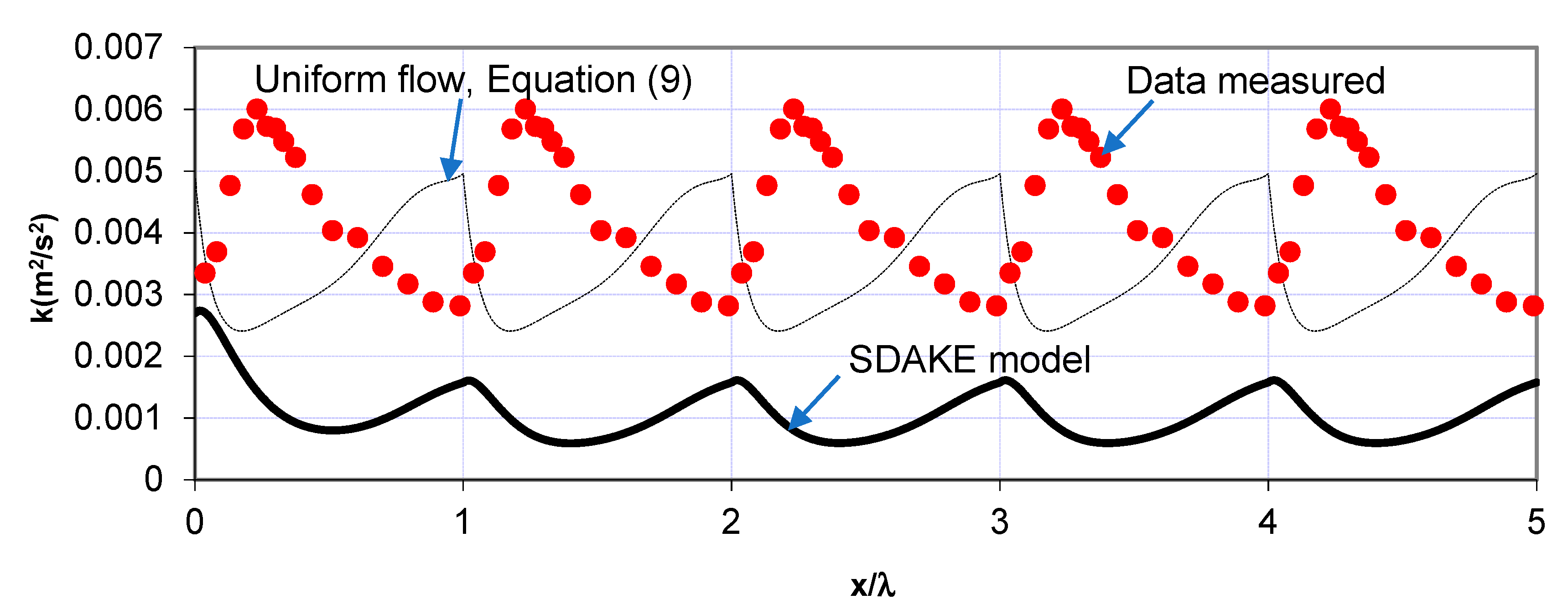
Figure 4 presents a comparison between the data and the calculated depth-averaged turbulent kinetic energy using the SDAKE model. The model’s results clearly appear to be out of phase with the measurements, as it predicts a maximum value near the crest and a minimum value around the point of reattachment. The disagreement with the measurements comes from the fact that the dominant production term in the model is related to the bed shear velocity, an assumption that is valid only for the case of uniform flow over a flat bed.

In the following subsection, a moment-based version of the k-ε model is presented to obtain better results than the SDAKE model for the cases of flow over a varying bed terrain.

3.3. A New Moment-Based Depth-Averaged k-ε (MDAKE) Model

Detailed measurements of turbulence over a train of fixed bedforms showed that the main contribution of the turbulence production is due to the strong free shear layer (generated downstream of the crest) and only a relatively small part comes from the internal boundary layer [19].

This means that the shear velocity is not a relevant scale for simulating the turbulence kinetic energy in this problem. Therefore, another velocity scale needs to be used to represent the strength in the shear layer or the average gradient of the velocity in the shear layer zone in the vertical plane. The idea presented here is based on a moment concept.

In the moment approach, the degrees of freedom in the model’s velocity profile are increased as each velocity profile is virtually converted to an equivalent linear velocity profile having the same moment of momentum around the mid-water depth. Following this idea, a new integral-moment velocity scale, $u_1$, could be defined and calculated using Equation (1).

Figure 3a shows a typical spatial variation in $u_1$ over one wavelength of a bedform. A large value of $u_1$ means that the average gradient in the velocity profile is large. Therefore, the new integral-moment velocity scale, $u_1$, could be used to express the strength of the shear layer and, consequently, the production of turbulence in the free shear zone.

It is interesting to notice that the location of maximum $\overline{k}$ (Figure 3b) lies downstream of the location of the maximum value of $u_1$, Figure 3a. This reveals that turbulence is mainly generated within the free shear layer and then transported downstream by the mean flow and this confirms that a sort of transport mechanism or equation is needed for modeling such a process.

As a first step of predicting $\overline{k}$ over bedforms, a one-equation model basically based on a version of depth-averaged k-equation was attempted. The main problem in the one-equation model is that the turbulent length scale should be assumed empirically [44]. Rifai and Smith [34] experimentally investigated the flow over a train of fixed triangular elements and they suggested that the macro-scale of turbulence is in the order of the height of the bed topography elements, not the flow water depth. Accordingly, the turbulent length scale in the k-equation is simply assumed to be a constant and is proportional to the bedform height. The resulted predictions showed that (figures are not presented here) the model significantly underpredicts the peak of the depth-averaged turbulent kinetic energy. This means that the turbulent length scale significantly changes over the bedform and it is incorrect to consider it as a constant through the spatial domain. Therefore, it was decided to move to the two-equation transport models, such as the k-ε equations.

In the proposed modification of the k-ε model, the depth-averaged production term could be represented as:

$${\rm P}\approx -\rho \overline{u\prime ·w\prime }\frac{\partial U}{\partial z}$$

(13)

By using the new integral-moment velocity, $u_1$, as a velocity scale, one can write:

$$\overline{-u\prime ·w\prime }~u_1^2\approx r\prime ·{\zeta }_k·u_1^2$$

(14)

r’ = r/2 is a constant (Equation (24)) and ${\zeta }_k$ is a calibration coefficient. Moreover, the velocity gradient could be approximated using a linear velocity assumption as:

$$\frac{\partial U}{\partial z}\equiv \frac{2·u_1}{h}$$

(15)

Therefore,

$$P\approx r·{\zeta }_k\frac{u_1^3}{h}$$

(16)

The value of the calibration coefficient $({\zeta }_{ko})$ in the case of uniform flow over a flatbed could be obtained from Equation (17) as follows:

$${\zeta }_{ko}=\frac{1}{r·{\alpha }^2{C}_{*}^2}$$

(17)

Similarly, the generation of a dissipation term can be formulated by assuming that the generation rate of ε is proportional to the production rate of k, which feeds the large-scale end of the spectrum [46,47].

The generation rate is:

$$\epsilon ~\frac{P}{t_s}=\frac{\epsilon }{k}P$$

(18)

where t_s represents the timescale of energy transported through the spectrum.

By using the new integral-moment velocity, $u_1$, as a velocity scale, one can write:

$$k~{u_1}^2$$

(19)

Realizing that dissipation may be scaled by large eddy parameters in the case of a high Reynolds number (i.e., existence of the inertial subrange spectrum), one can write dissipation as [46,47].

ε ~ u₁ ³/ℓ

(20)

where ℓ represents the average size of the most energetic eddies (ℓ/h ≈ Δ/h ≈ 0.1–0.3). Finally, the generation rate of ε can be reduced to:

Generation rate of

$$\epsilon \approx \frac{\Phi ·C_{\epsilon }·u_1^4}{h^2}$$

(21)

$$U_o\frac{\partial \overline{k}}{\partial x}=\frac{r·{\zeta }_k·u_1^3}{h}+2·C_{\mu }{\left(\frac{\partial U_o}{\partial x}\right)}^2\frac{{\overline{k}}^2}{\overline{\epsilon }}-\overline{\epsilon }$$

(22)

$$U_o\frac{\partial \overline{\epsilon }}{\partial x}=\frac{\Phi ·C_{\epsilon }·u_1^4}{h^2}+2·C_{1\epsilon }·C_{\mu }{\left(\frac{\partial U_o}{\partial x}\right)}^2\overline{k}-C_{2\epsilon }\frac{{\overline{\epsilon }}^2}{\overline{k}}$$

(23)

where:

R, F and a are dimensionless coefficients (in the following subsection, a discussion will be given in the next subsection to present how to determine their values).

κ is the von Karman constant (κ = 0.41).

The new moment-based k-ε model, Equations (22) and (23), are similar to the SDAKE model, except for the production of turbulence, the first term in the right-hand side of Equation (22), and the generation of dissipation, the first term in the right-hand side of Equation (23). Close inspection of Equation (22) shows that it represents a balance between the energy convection, energy production and viscous dissipation. It should be mentioned that the energy production due to the spatial gradient of the downstream velocity, the second term in the RHS of Equations (22), is significantly small compared to the dominant production due to the free shear layer, the first term in the RHS of Equation (22). Therefore, the second term in the RHS of Equation (22) and its corresponding term in Equation (23) are neglected in this study. Further, the diffusion contribution is neglected. This assumption is based on Nakagawa and Nezu’s findings [29] while studying the balance of turbulent energy for the case of turbulent water flow past a negative step, a problem that is quite similar to the current study.

3.4. Model Descritization

3.4.1. Preface

The 1D k-ε model (whether SDAKE or MDAKE) forms a typical steady-state set of transport equations. The convective terms for the equations are discretized using the first-order backward upwinding scheme.

Using a first-order upwinding scheme has, on the one hand, the advantage of simplicity to implement, and the scheme is stable and not oscillating. On the other hand, the scheme is first-order accurate and it is dissipative.

Using a suitable fine discretization value for ∆x can minimize the expected numerical diffusion and reduce the corresponding truncation error. In this study, for instance, a typical value of ∆x = 0.002 m is used for T5 and T6 experiments (refer to the calibration section), which corresponds to a discretization intensity index of (λ/∆x) = 800.

3.4.2. GCI

In order to examine whether the used ∆x is quite small or not, the Grid Conversion Index (GCI) is applied for the assessment of the quality of mesh discretization. The grid convergence index (GCI) is a relatively new discretization error estimation technique. The GCI is calculated to answer whether the adopted mesh in the simulation is refined enough or not [48]. A minimum of two mesh solutions is required, but three is recommended to calculate the GCI.

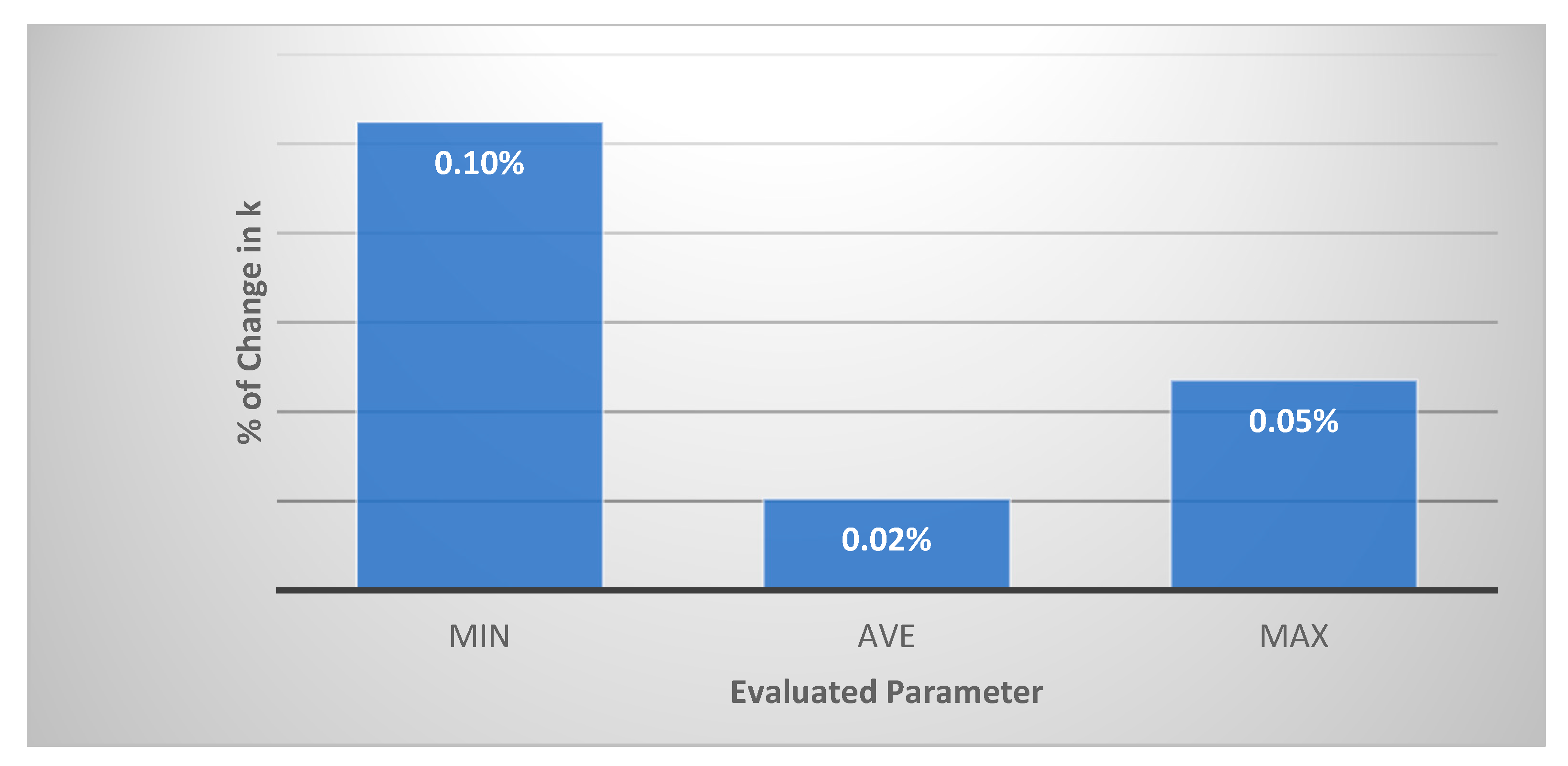
In this study, three mesh sizes are used to calculate the GCI. The sizes range from coarse to medium (the size adopted in the study) and then to fine. The sizes are (for experiments T5 and T6): 0.004 m, 0.002 m and 0.001 m, corresponding to λ/∆x values of 400, 800 and 1600, respectively. The assessment will track three variables: maximum, average and minimum depth-averaged turbulent kinetic energy throughout the whole train of bedforms. The following figure shows a snap shot of the GCI analysis.

Based on the GCI results shown in Figure 5, it is found that decreasing the mesh size from medium to fine will result in a change in the maximum $\overline{k}$ of only 0.05%. This means that adopting the medium-size mesh is quite sufficient.

4. Calibration of MDAKE Model

4.1. Introduction

The MDAKE model introduces a new velocity scale, u₁, that is important for the evaluation of the production and generation of turbulent kinetic energy and dissipation rate, respectively. The model equations (Equations (22) and (23)) contain a number of dimensionless coefficients r, Φ and ξ_k. Some of these coefficients can be determined analytically, whereas others require the use of measurements for calibration.

The role of the coefficients r and Φ is to force the MDAKE model to correctly predict the true depth-averaged turbulent kinetic energy if the model is applied for the benchmark case of uniform flow over a flat bed. Therefore, r and Φ can be determined by forcing Equations (22) and (23) to reduce to Equation (8) for the uniform flow case.

It should be emphasized that the expressions of both r and $\Phi$ coefficients are chosen to be interconnected with each other in a way that fulfills the following two objectives if the flow is turned out to be uniform over a flatbed:

-

The depth-averaged value of k automatically reduces to the true value of k for the benchmark case of uniform flow over a flatbed;

-

The solution of k becomes independent on the value of the coefficient ζ_k.

The following equations (Equations (24) and (25)) provide an estimation for the dimensionless coefficients r and Φ, respectively.

$$r=\sqrt{2.067C_r\frac{C_{\epsilon }}{C_{2\epsilon }}}$$

(24)

$$\Phi ={(C_{*}\alpha {\xi }_k)}^2$$

(25)

The coefficient α in Equation (25) provides the ratio between the integral velocity, $u_1$, and the mean velocity, U_o, in the case of uniform flow over a flat bed [3]. It is known that the log-law could be used to predict the velocity profile in the inner region in the case of uniform flow. Therefore, α can be obtained using the following equation.

$$\alpha =C_{\alpha }\frac{1.5}{C_{*}\kappa }$$

(26)

If the log-law is applied over the whole water depth, the coefficient C_α is found to be very close to 1. A more accurate way to get the coefficient C_α is to assume a log-wake relation, which gives a value of C_α = (1 + 8 Π/π²), where Π is the wake parameter and has a range from 0 to 0.2. Nezu and Rodi found that Π remains nearly constant and equals 0.2 when the Reynolds number is larger than 10⁵ [49]. However, it should be mentioned that there is no specific and accurate relation to calculate the wake parameter, Π. For the upper value of Π = 0.2, the corresponding upper value of C_α is ≈1.16.

In the section to follow, the modified model will be calibrated in order to estimate the dimensionless coefficient, ξ_k.

4.2. Lab Experiments for Model Calibration

The new k-ε model to be presented in the next subsections requires flow measurements for calibration.

Table 1. Summary of the geometrical and flow parameters of selected fixed-bedform experiments reported in the literature.

	T5 (1)	T6 (1)	Run2 (2)	Run3 (2)	Run4 (2)	Run5 (2)	Run6 (2)	Lyn2 (3)	Lyn3 (3)	Bennett (4)
λ (m)	1.60	1.60	0.80	0.80	0.40	0.40	0.40	0.15	0.15	0.63
∆ (m)	0.080	0.080	0.040	0.040	0.040	0.040	0.040	0.012	0.012	0.040
hav (m)	0.252	0.334	0.158	0.546	0.159	0.159	0.300	0.061	0.061	0.120
∆/h	0.317	0.240	0.253	0.073	0.252	0.252	0.133	0.197	0.197	0.333
∆/λ	0.050	0.050	0.050	0.050	0.100	0.100	0.100	0.080	0.080	0.063
Fn	0.25	0.28	0.30	0.12	0.30	0.16	0.31	0.35	0.71	0.44
ku (m2/s2)	0.00281	0.00371	0.00226	0.00071	0.00305	0.00100	0.00430	0.00159	0.00571	0.00320
ζk	0.004	0.009	0.014	0.020	0.008	0.009	0.025	-	-	0.019

⁽¹⁾ Van Mierlo and de Ruiter [50]; ⁽²⁾ Mclean et al. [51], ⁽³⁾ Lyn [52]; ⁽⁴⁾ Bennett, and Best [53].

lists the flow parameters and bed geometry of the selected experiments of water flow over a train of fixed bedforms that are available in the literature and to be used in this study. Most of these laboratory experiments are for transitional roughness surfaces where the dimensionless sand grain roughness lies between 5 and 70. The dimensionless Chezy coefficient ($C_{*}$) ranges from 15 to 20. The steepness ratio (∆/λ) ranges from 1/10 to 1/20, and the crest-height-to-water-depth ratios (∆/h) range from 0.07 to 0.3, with the Froude number (F_n) varying from 0.12 to 0.71 and a channel width (b) that varies from 0.08 to 1.5 m.

4.3. Calculation of $\overline{k}$ from Experimental Data

In order to compute the turbulent kinetic energy field from the turbulence measurements (for experiments listed in Table 1), all the components of the turbulent velocity in the three coordinates should be known, as shown in Equation (3). Unfortunately, the available laboratory experiments for flow over bedforms generally provide turbulence data for only the streamwise and the vertical components. The lateral, the spanwise, component is unknown. One way to predict the lateral turbulent component is to claim isotropic conditions, which means that $\sqrt{\overline{v^{\prime 2}}}=\sqrt{\overline{u^{\prime 2}}}$. However, this might be regarded as a crude assumption. Another approach is to assume that the spanwise turbulence values approximately equal the vertical turbulence values, i.e., $\sqrt{\overline{v^{\prime 2}}}=\sqrt{\overline{w^{\prime 2}}}$. Mendoza and Shen [28] proposed this assumption while comparing their 2D–k-ε numerical model with Raudivi’s experiment of flow over a train of ripples.

In the case of uniform flow over a flat bed, it is observed that $\sqrt{\overline{u^{\prime 2}}}>\sqrt{\overline{v^{\prime 2}}}>\sqrt{\overline{w^{\prime 2}}}$ [50]. Based on this observation, a third approach is to assume that the spanwise turbulence values lie midway between the streamwise and the vertical turbulence values. Song and Chiew [54] carried out 3D turbulent measurements using a 3D acoustic Doppler velocimeter in cases of nonuniform (accelerating/decelerating) open-channel flow. Their also data showed that the dimensional spanwise turbulent intensity lies in the midway between the corresponding values in the other two directions and the spanwise component equals to the average of the other two components, Equation (27). This approach was followed before by Van Mierlo and de Ruiter [50], who used Equation (27) to calculate k over a train of fixed bedforms. In 1985, Driver and Seegmiller [55] applied Equation (28) to obtain the distribution of the turbulent kinetic energy for airflow over a rearward-facing step. Nakagawa and Nezu [29] also used the same assumption to quantify the turbulent energy diffusion term in the turbulent energy balance equation while studying the structure of turbulent flow over a negative step. Siddiqui and Loewen [56] suggested to use Equation (28) to get the turbulent kinetic energy field for the microscale breaking waves that were generated by the influence of wind waves.

$$\sqrt{\overline{v^{\prime 2}}}=\left(\frac{1}{2}[\sqrt{\overline{u^{\prime 2}}}+\sqrt{\overline{w^{\prime 2}}}]\right)$$

(27)

$$v^{\prime 2}=\left(\frac{1}{2}\left[u^{\prime 2}+w^{\prime 2}\right]\right)$$

(28)

One possible way to assess the validity of the assumptions given by Equations (27) or (28) (within the depth-averaging framework) is to look at the recent highly accurate direct numerical simulation (DNS) results that are available for similar applications. In 2009, Bhaganagar and Hsu [57] conducted a DNS study for flow over a set of 2D and 3D wave ripples. Based on their available data, it is possible to calculate two values for the depth-averaged turbulent kinetic energy. The first value is directly obtained from the measurements and this will possibly provide the true value of $\overline{k}$ (from the DNS perspective) and the second value is obtained partly from the DNS measurement and by applying the approximation given by Equation (27).

Table 2. Comparison of depth-averaged turbulent kinetic energy calculation.

Simulation Run	$\overline{k}$	$\overline{k}$*	% of Variance
2D ripples (Ret = 180)	5.04	5.58	11%
2D ripples (Ret = 400)	6.58	7.05	7%

* Approximate value calculated using Equation (27).

, below, shows the summary of the results of two different NDS runs for flow over 2D ripples, where R_eτ is the Reynolds number based on the bed shear velocity. The table shows that adopting the assumption (given by Equation (27)) tends to overpredict the actual depth-averaged value by 7 to 11%. Despite the crudeness of the assumption but because of the depth-averaging process, it tends to reduce its effect on the calculated averaged value.

In this study, Van Mierlo’s proposal [50] will be applied and Equation (27) will be adopted.

It is also expected that assuming the lateral turbulence component will not significantly affect the trend of the spatial distribution of $\overline{k}$ but it might affect the amplitude and that could change the values in the calibration coefficient, ξ_k.

In order to account for the above-mentioned variance that is introduced by adopting Equation (27), a minus error bar (equivalent to the maximum variance shown in Table 2) is added to the measurements, as shown in Figure 6.

4.4. Model Calibration

Before calibrating the new model (Equations (22) and (23)), the spatial variables, h, U_o and $u_1$, should be determined. Despite the fact these variables could be calculated using VAM models (similar to [58,59,60,61,62]), in this work, they were derived from the measurements and were best fitted using spline curves. Via the spline curves, the spatial variations in h, U_o and $u_1$ were determined over the bedform wavelength.

Then $\overline{k}$ and $\overline{\epsilon }$ were calculated numerically using a simple first-order finite difference scheme. The spatial discretization, dx, was chosen to be quite small, dx = 0.0005 m, to decrease the effect of the artificial diffusion. A calculation domain consisting of a train of five bedforms is considered assuming the turbulent flow to be fully developed over each bedform. Accordingly, the flow variables will be repeated in a cyclic pattern through the domain. Then, Equations (22) and (23) were used to predict the corresponding depth-averaged turbulent kinetic energy and dissipation rate. The calibration coefficient, ξ_k, is adjusted in order to get the best match with the experimental data. The value of ξ_k for each experiment is given in Table 1.

5. Results and Discussion

5.1. Uniform Flow over Flatbed BenchMark Case

As the SDAKE model does not give the true depth-averaged values for the turbulent kinetic energy, it is of interest to know how the virtual values, $\tilde{k}$, differ from the true ones, $\overline{k}$. A simple way to do that is to use the SDAKE model (Equations (10) and (11)) to predict the turbulent kinetic energy for the case of uniform flow over a flat bed. In the case of uniform flow over a flat bed, all the spatial derivatives in Equations (10) and (11) can be dropped and, consequently, the two equations can be reduced to:

$${\frac{\tilde{k}}{u_{*}^2}|}_{UniformFlow}=\frac{C_{2\epsilon }·C_{*}^2}{C_{\epsilon }}$$

(29)

This can be further reduced using Equation (12) to:

$${\frac{\tilde{k}}{u_{*}^2}|}_{UniformFlow}=\frac{1}{3.6}\sqrt{\frac{C_{*}}{C_{\mu }}}$$

(30)

By comparing Equations (9) and (30), one can find that $\tilde{k}\approx \left(1.5-2.3\right)\overline{k}$ for the case of uniform flow over a flat bed. This means that the virtual values for $\tilde{k}$ estimated by SDAKE models tend to be higher than the true depth-averaged values $\overline{k}$, and SDAKE models tend to overestimate the true values in the depth-averaged turbulent kinetic energy $\overline{k}$ by 50% to 130% for the uniform flow over a flatbed benchmark case. For the idealized smooth bed case ($C_{*}$ = 10), the overestimation will be in the order of 50%, whereas for the very rough surfaces ($C_{*}$ = 20), the overestimation will be in the order of 130%.

5.2. Nonuniform Flow over a Train of Bedforms Case

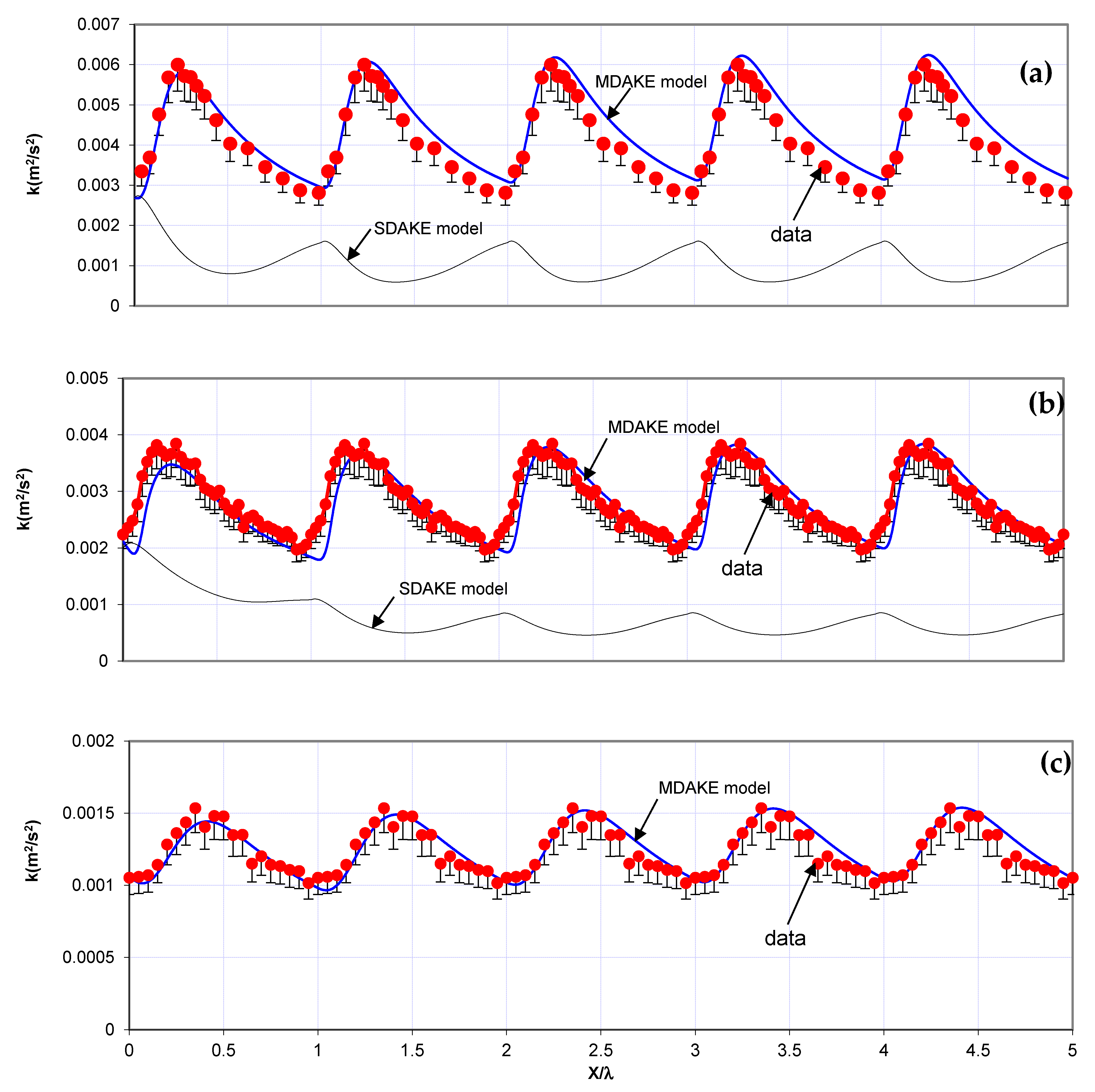
Figure 6a presents the spatial distribution of $\overline{k}$ over a train of five bedforms for experiment T5. It is noticed that the new model after calibration predicts the location of $\overline{k}$ max reasonably well and the predictions of the model are generally in good agreement with the measurements.

Figure 6b shows a comparison between the measured and the predicted values of $\overline{k}$ for the experiment (Run2). The prediction of the $\overline{k}$ max position seems to be slightly shifted downstream.

The results for experiment (Run5) are given in Figure 6c. Very good agreement is found between the measurements and the predictions after calibration.

Figure 7 presents the spatial variation in the eddy viscosity coefficient, Fν_t, (Equation (29)) over one wavelength of a bedform. It is interesting to notice that Fν_t is somewhat larger than the values reported in the case of uniform flow over a flat bed (Fν_t = 0.06–0.07). The large values of Fν_t (shown on Figure 7) generally refer to the large values for the flow eddy viscosity for the case of flow over bedforms (that is characterized by the existence of flow separation and high shear flow zones downstream of the crest) compared to the case of uniform flow over a flat bed.

Fν_t could be determined using the following equations:

$${\nu }_t=C_{\mu }·\frac{k^2}{\epsilon }$$

(31)

$$F_{\nu t}=\frac{{\nu }_t}{h·U_o/C_{*}}$$

(32)

where ν_t is the depth-averaged eddy viscosity, C_μ is a constant and equals 0.09.

The data shown in Figure 7 were produced from the T5 experiment [50], whereas the predictions (shown as solid black line) were obtained via Equations (31) and (32) of the MDAKE model. Good agreement was found between the measurements and the predictions of the new k-ε model.

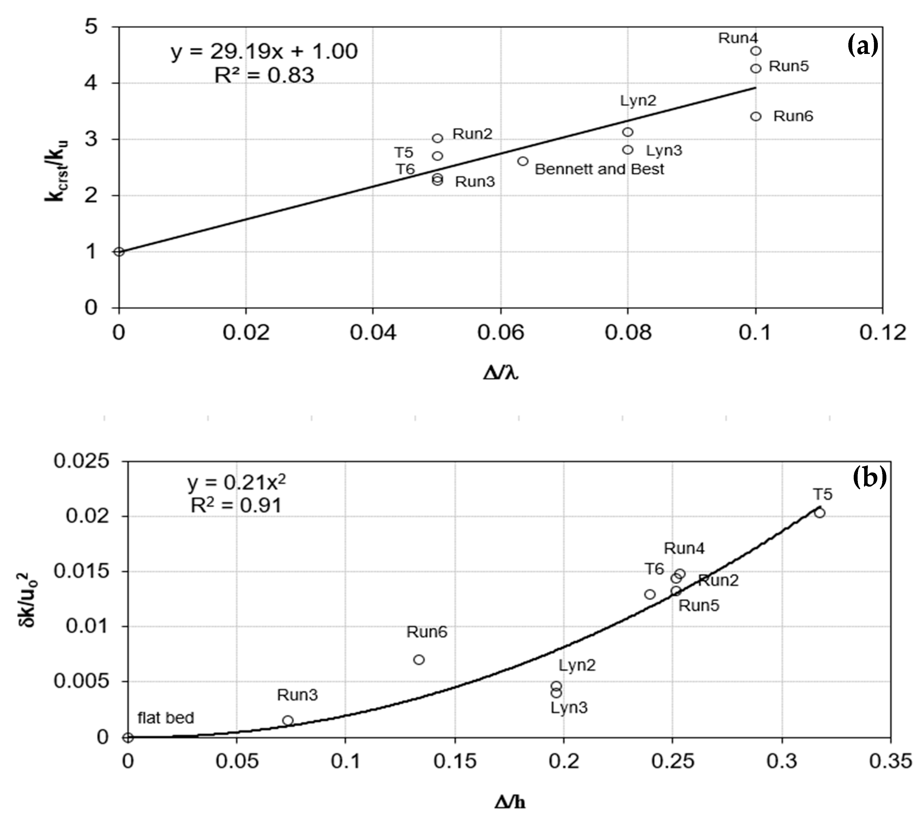
Figure 8a shows the effect of the bedform height and steepness on the depth-averaged turbulent kinetic energy over the crest at equilibrium conditions. The curve intersects the vertical axis at a value of unity, which is the case for a flatbed. As the steepness or the height of the bedform increases, the ratio ${\overline{k}}_{crst}/\overline{k_u}$ increases over unity and it reaches an average value of almost 2.5 for ∆/λ = 0.05, Figure 8a. This increase can be justified as follow: for a given water depth, as the bedform height increases, the resulting shear layer zone becomes larger and stronger. Consequently, more turbulence will be generated and transported downstream with the mean flow, causing ${\overline{k}}_{crst}/\overline{k_u}$ to increase.

Many researchers found that the bed roughness height tends to decrease the x-turbulence intensity [30]. The previous statement does not contradict Figure 8a. While bedforms can be considered as mega-roughness elements, their effects on the structure of the flow are different from the natural bed roughness particles (skin roughness) because of the existence of flow separation and the strong shear layer downstream of the crest.

As a result of flow separation downstream of the crest, strong shear layer flow exists and produces turbulence. Figure 8b describes the net increase in the depth-averaged turbulent kinetic energy, δk, over the bedform as a function of the ratio ∆/h; refer to Figure 3b for definition.

5.3. Limitations of the MDAKE Model

One of the drawbacks of the new MDAKE model is its dependence on the wake coefficient C_α. As was discussed before in Section 4.1, this coefficient depends on the wake parameter, Π; unfortunately, there is no specific universal and accurate relation to describe this parameter. However, it is noticed that C_α might range from a minimum value of 1 and a maximum value not larger than 1.2. The laboratory experiments used in this study suggest a value for C_α closer to 1.15. It was noticed that most of the experimental runs produce a good match with the data for C_α = 1.15 and one run (run2) provides a good match at C_α = 1.0. Nevertheless, more laboratory experiments are required to investigate the factors that affect C_α.

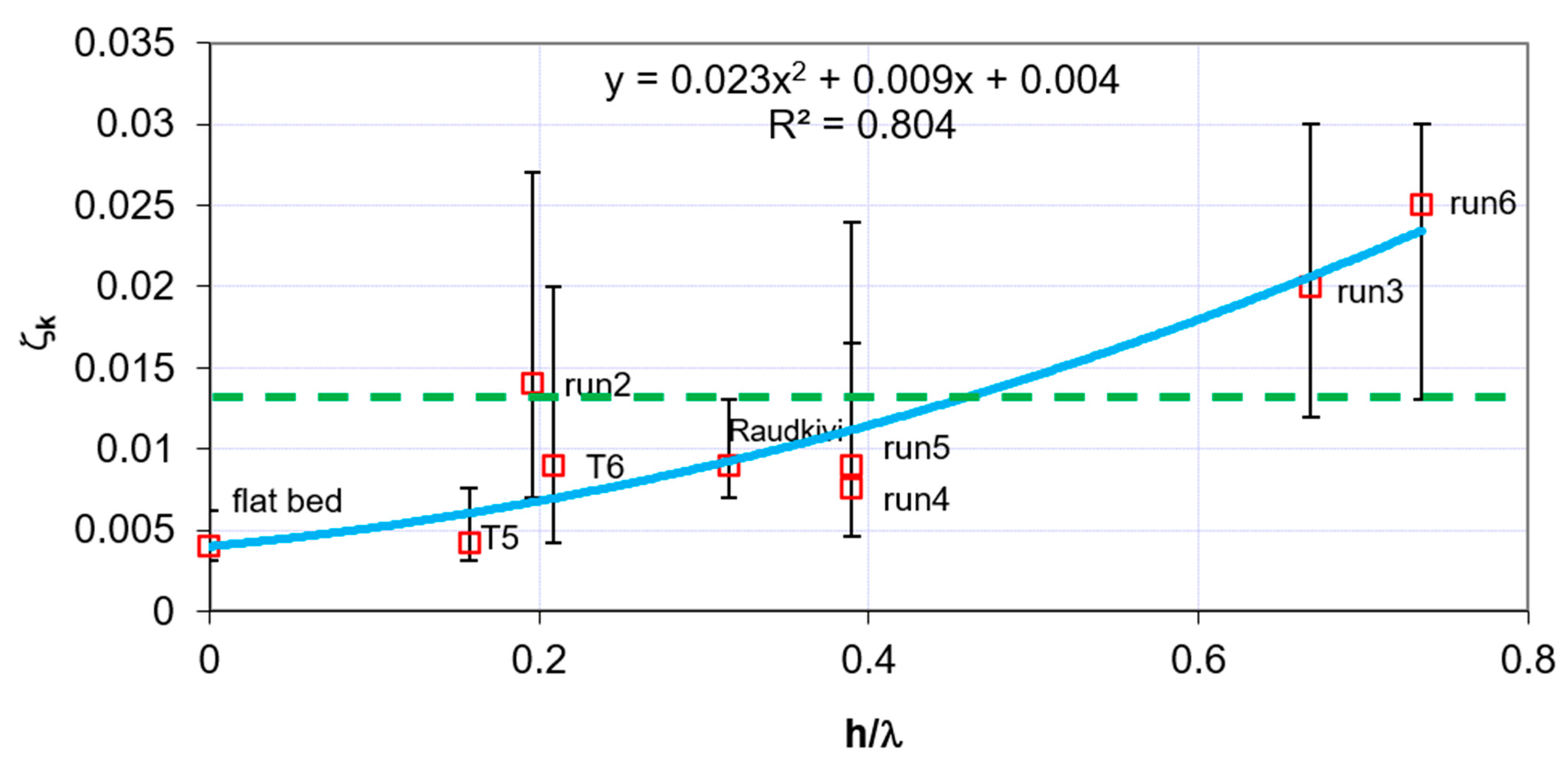
Figure 9 describes the outcome of the calibration in the MDAKE model with the laboratory experiments. The calibration coefficient, ξ_k, varies from about 0.004 to 0.025 and it can be related with the depth to wavelength ratio, h/λ, via a parabolic relation, as shown on Figure 8. It should be mentioned that the proposed relation also satisfies the uniform flow case over a flatbed (the intersection point with the vertical axis).

In Figure 9, three values of ξ_k are presented for each experiment: the medium value, which gives a good match with the data, the upper limit value of each bar, which gives, at most, 25% over-prediction of k_max and finally, the lower limit value, which gives, at most, 20% under-prediction of k_max.

It is of interest to investigate how much discrepancy will be produced upon using a global constant value of ξ_k for all the experiments. Figure 9 suggests a global value of about ξ_k = 0.013, as shown by the dashed line. Figure 10a–f presents the predictions of the MDAKE model using this global constant value for the calibration coefficient for all the experiments (ζ_k = 0.013). In general, good agreement is still obtained, except for experiment T5, where the model appears to over-predict kmax by about 50%. Despite this, it is interesting to notice that the model generally provides good predictions for $\overline{k}$ over the crest.

It should also be mentioned that the ratio of h/λ for fully developed bedforms is expected to be less than 0.4. This might suggest using a calibration coefficient that best fit only the experiments within this range. According to Figure 9, a value of (ζ_k = 0.075) might be more suitable.

6. Conclusions and Challenges

A 1-D depth-averaged k-ε model (based on the moment concept, MDAKE) was introduced to predict the depth-averaged turbulent kinetic energy for a fully developed turbulent flow over train bedforms. The MDAKE model makes use of the integral-moment velocity scale ($u_1$) to provide better estimates for the production of turbulent kinetic energy and also for the generation of energy dissipation. Due to the use of irrelevant velocity scales, the current study showed that the standard depth-averaged k-ε (SDSKE) model could overestimate the depth-averaged turbulent kinetic energy for the benchmark uniform flow case over a flatbed by 130% and the SDAKE model predictions also produce out-phase results of $\overline{k}$ for the varying bed topography cases. That said, the skin friction bed shear velocity cannot be used to describe the turbulent production in the vertical plane in the case of flow over bedforms as the majority of the turbulent production is due to the free shear layer zone that comes out of separation. Accordingly, the moment approach was proposed to provide the model with a relevant velocity scale, $u_1$, which can be used to describe the dominant production term in the problem. The model was calibrated using a number of laboratory experiments chosen from the literature. It was found that the calibration coefficient appears to increase as h/λ increases. It is noticed that a global constant value of 0.013 generally seems to give reasonable results for almost all the tested experiments within a range of (0 < h/λ ≤ 0.72). A lower value of 0.0075 might also be used for equilibrium bedforms, where (h/λ ≤ 0.4).

The new 1D MDAKE model could be extended to a 2D depth-averaged version. In this case, the lateral integral moment velocity scale ($v_1$) might be used in conjunction with the downstream integral moment velocity scale ($u_1$) to describe the generation terms in each direction. More effort needs to be made to determine the factors affecting the calibration parameters (ξ_k) in such a case.

It should be clearly mentioned that the proposed k-ε MDAKE model was not examined for the cases of developing flow and non-equilibrium turbulent conditions. Further studies are needed to assess the model in such conditions.

This study is considered an important step towards extending the validity of the depth-averaged flow models to be used in more complicated applications and it will help in obtaining better predictions (using the depth-averaged models) for different applications, including sediment transport, bedform evolution and water quality and mixing of contaminants in rivers.

References

1. Sarchani, S.; Seiradakis, K.; Coulibaly, P.; Tsanis, I. Flood inundation mapping in an ungauged basin. Water 2020, 16, 1532. [Google Scholar] [CrossRef]
2. Ongdas, N.; Akiyanova, F.; Karakulov, Y.; Muratbayeva, A.; Zinabdin, N. Application of HEC-RAS (2D) for flood hazard maps generation for Yesil (Ishim) river in Kazakhstan. Water 2020, 12, 2672. [Google Scholar] [CrossRef]
3. Elgamal, M. A Moment-Based Chezy Formula for Bed Shear Stress in Varied Flow. Water 2021, 13, 1254. [Google Scholar] [CrossRef]
4. Elgamal, M.H.; Steffler, P.M. A Bed Stress Model for Non-Uniform Open Channel Flow. In Proceedings of the 15th Hydrotechnical Conference, CSCE, Vancouver, BC, Canada, 30 May–2 June 2001. [Google Scholar]
5. Steffler, P.M.; Jin, Y.C. Depth averaged and moment equations for moderately shallow free surface flow. J. Hydraul. Res 1993, 31, 5–17. [Google Scholar] [CrossRef]
6. Avramenko, A.; Hamalainen, J. Two-dimensional depth-averaged model simulation. In AIP Conference Proceedings; AIP Publishing LLC: Melville, NY, USA, 2015; Volume 1648, p. 850017. [Google Scholar]
7. Sanchez, A.; Wu, W.; Beck, T.M. A depth-averaged 2-D model of flow and sediment transport in coastal waters. Ocean. Dyn. 2016, 66, 1475–1495. [Google Scholar] [CrossRef]
8. Bai, F.; Yang, Z.; Huai, W.; Zheng, C. A depth-averaged two dimensional shallow water model to simulate flow-rigid vegetation interactions. Procedia Eng. 2016, 154, 482–489. [Google Scholar] [CrossRef]
9. Kang, L.; Jing, Z. Depth-averaged non-hydrostatic hydrodynamic model using a new multithreading parallel computing method. Water 2017, 9, 184. [Google Scholar] [CrossRef] [Green Version]
10. Papa, M.N.; Sarno, L.; Vitiello, F.S.; Medina, V. Application of the 2D depth-averaged model, FLATModel, to pumiceous debris flows in the Amalfi Coast. Water 2018, 10, 1159. [Google Scholar] [CrossRef] [Green Version]
11. Lai, Y.G. A two-dimensional depth-averaged sediment transport mobile-bed model with polygonal meshes. Water 2020, 12, 1032. [Google Scholar] [CrossRef] [Green Version]
12. Wang, W.; Martin, T.; Kamath, A.; Bihs, H. An improved depth-averaged nonhydrostatic shallow water model with quadratic pressure approximation. Int. J. Numer. Methods Fluids 2020, 92, 803–824. [Google Scholar] [CrossRef] [Green Version]
13. Rastogi, A.; Rodi, W. Prediction of Heat and Mass Transfer in Open Channels. J. Hyd. Div. ASCE 1978, 97, 397–420. [Google Scholar] [CrossRef]
14. Yu, L.; Righetto, A.M. Depth-averaged turbulence k–w model and applications. Adv. Eng. Softw. 2001, 32, 375–394. [Google Scholar] [CrossRef]
15. Wu, W.; Wang, P.; Chiba, N. Comparison of five depth-averaged 2-D turbulence models for river flows. Arch. Hydro-Eng. Environ. Mech. 2004, 51, 183–200. [Google Scholar]
16. Fe, J.; Navarrina, F.; Puertas, J.; Vellando, P.; Ruiz, D. Experimental validation of two depth-averaged turbulence models. Int. J. Numer. Methods Fluids 2009, 60, 177–202. [Google Scholar] [CrossRef]
17. Duan, J.G.; Nanda, S.K. Two-dimensional depth-averaged model simulation of suspended sediment concentration distribution in a groyne field. J. Hydrol. 2006, 327, 426–437. [Google Scholar] [CrossRef]
18. Nelson, J.M.; Mclean, S.R.; Wolfe, S.R. Mean Flow and Turbulence Fields Over Two-Dimensional Bed Forms. Water Resour. Res. 1993, 29, 3935–3953. [Google Scholar] [CrossRef]
19. Nelson, J.M.; Shreve, R.L.; Mclean, S.R.; Drake, T.G. Role of Near-bed Turbulence Structure in Bed Load Transport and Bed Form Mechanics. Water Resour. Res. 1995, 31, 2071–2086. [Google Scholar] [CrossRef]
20. Mclean, S.R.; Nelson, J.M.; Wolfe, S.R. Turbulence structure over two-dimensional bed forms: Implications for sediment transport. J. Geophys. Res. 1994, 99, 12729–12747. [Google Scholar] [CrossRef]
21. Lee, H.; Ha, M.Y.; Balachandar, S. Work-based criterion for particle motion and implication for turbulent bed-load transport. Phys. Fluids 2012, 24, 116604. [Google Scholar] [CrossRef]
22. Ali, S.Z.; Dey, S. Bed particle saltation in turbulent wall-shear flow: A review. Proc. R. Soc. A 2019, 475, 20180824. [Google Scholar]
23. Barati, R.; Neyshabouri, S.A.A.S.; Ahmadi, G. Issues in Eulerian–Lagrangian modeling of sediment transport under saltation regime. Int. J. Sediment Res. 2018, 33, 441–461. [Google Scholar] [CrossRef]
24. Radice, A.; Nikora, V.; Campagnol, J.; Ballio, F. Active interactions between turbulence and bed load: Conceptual picture and experimental evidence. Water Resour. Res. 2013, 49, 90–99. [Google Scholar] [CrossRef] [Green Version]
25. Paiement-Paradis, G.; Marquis, G.; Roy, A. Effects of turbulence on the transport of individual particles as bedload in a gravel-bed river. Earth Surf. Processes Landf. 2011, 36, 107–116. [Google Scholar] [CrossRef]
26. Zgheib, N.; Fedele, J.J.; Hoyal, D.C.J.D.; Perillo, M.M.; Balachandar, S. Direct numerical simulation of transverse ripples part ii. self-similarity, bedform coarsening, and effect of neighbouring structures. J. Geophys. Res. Earth Surf. 2018, 123, 448–477. [Google Scholar] [CrossRef]
27. Guan, L.; Salinas, J.S.; Zgheib, N.; Balachandar, S. The role of bed-penetrating Kelvin–Helmholtz vortices on local and instantaneous bedload sediment transport. J. Fluid Mech. 2021, 911, A50-1-14. [Google Scholar] [CrossRef]
28. Yang, J.Q.; Nepf, H.M. A turbulence-based bed-load transport model for bare and vegetated channels. Geophys. Res. Lett. 2018, 45, 10–428. [Google Scholar] [CrossRef]
29. Nakagawa, H.; Nezu, I. Experimental Investigation on Turbulent Structure of Backward-Facing Step Flow in an Open Channel. J. Hydr. Res. 1987, 25, 67–88. [Google Scholar] [CrossRef]
30. Nezu, I.; Nakagawa, H. Turbulence in Open-Channel Flows; Balkema, A.A., Ed.; Routledge: Rotterdam, The Netherland, 1993. [Google Scholar]
31. Grass, A.J. Structural features of turbulent flow over smooth and rough boundaries. J. Fluid Mech. 1971, 50, 233–255. [Google Scholar] [CrossRef]
32. Lu, J.Y.; Chen, J.Y.; Hong, J.H.; Lu, T.F.; Liu, C.S. Turbulence Intensities of Shallow Rain-Impacted Flow over Rough Bed. J. Hydr. Engrg. ASCE 2001, 127, 881–886. [Google Scholar] [CrossRef]
33. Raudkivi, A.J. Study of Sediment Ripple Formation. ASCE J. Hydr. Div. 1963, 89, 15–33. [Google Scholar] [CrossRef]
34. Rifai, M.F.; Smith, K.V.H. Flow over Triangular Elements Simulating Dunes. J. Hyd. Div. 1971, 97, 963–976. [Google Scholar] [CrossRef]
35. Nelson, J.M.; Smith, J.D. Mechanics of Flow over Ripples and Dunes. J. Geophys. Res. 1989, 94, 8146–8162. [Google Scholar] [CrossRef]
36. Johns, B.; Soulsby, R.L.; Xing, J. A Comparison of Numerical Experiments of Free Surface Flow over Topography with Flume and Field Observations. J. Hydr. Res. 1993, 31, 215–228. [Google Scholar] [CrossRef]
37. Peric, M.; Ruger, M.; Scheuerer, G. Calculation of the Two-Dimensional Turbulent Flow over a Sand Dune Model; University of Erlangen: Erlangen, Germany, 1988; Rep. No. SRR-TN-88-O2. [Google Scholar]
38. Michelassi, V. Testing of Turbulence Models with an Artificial Compressibility Solution Method; University of Karlsruhe: Karlsruhe, Germany, 1989; Rep. SFB 210/T/49. [Google Scholar]
39. Mendoza, C.; Shen, H.W. Investigation of Turbulent Flow over Dunes. J. Hydr. Engrg. ASCE 1990, 116, 459–477. [Google Scholar] [CrossRef]
40. Sajjadi, S.G.; Aldridge, J.N. Prediction of Turbulent Flow over Rough Asymmetrical Bed Forms. Appl. Math. Model. 1995, 19, 139–152. [Google Scholar] [CrossRef]
41. Lefebvre, A. Three-dimensional flow above river bedforms: Insights from numerical modeling of a natural dune field (Río Paraná, Argentina). J. Geophys. Res. Earth Surf. 2019, 124, 2241–2264. [Google Scholar] [CrossRef]
42. McGuirk, J.J.; Rodi, W. A depth-averaged mathematical model for the near field of side discharges into open-channel flow. J. Fluid Mech. 1978, 86, 761–781. [Google Scholar] [CrossRef]
43. Launder, B.E.; Spalding, D.B. The numerical computation of turbulent flows. In Numerical Prediction of Flow, Heat Transfer, Turbulence and Combustion; Pergamon: Oxford, UK, 1983; pp. 96–116. [Google Scholar]
44. ASCE Task Committee on Turbulence Models in Hydraulic Computations. Turbulence Modeling of Surface Water Flow and Transport: Part I&II. J. Hydr. Engrg. 1988, 114, 970–991. [Google Scholar]
45. Kundu, P.K.; Cohen, I.M.; Dowling, D.R. Fluid Mechanics; Academic Press: Cambridge, MA, USA, 2015. [Google Scholar]
46. Wilson, J.D. Review of Turbulence Energy Closure Models for Momentum Transport, Lecture Notes; University of Alberta: Edmonton, AB, Canada, 2001. [Google Scholar]
47. Pinard, J.J.; Wilson, J.D. First-and second-order closure models for wind in a plant canopy. J. Appl. Meteorol. 2001, 40, 1762–1768. [Google Scholar] [CrossRef]
48. Journal of Fluids Engineering Editorial Policy, Statement on the Control of Numerical Accuracy. Available online: https://www.asme.org/wwwasmeorg/media/resourcefiles/shop/journals/jfenumaccuracy.pdf (accessed on 24 June 2022).
49. Nezu, I.; Rodi, W. Open-Channel Flow Measurements With A Laser Doppler Anemometer. J. Hydr. Engrg. ASCE 1986, 112, 335–355. [Google Scholar] [CrossRef]
50. Van Mierlo, M.C.L.M.; de Ruiter, J.C.C. Turbulence Measurements above Artificial Dunes. Delft Hydraul. 1988, 1–2, Q789. [Google Scholar]
51. Mclean, S.R.; Wolfe, S.R.; Nelson, J.M. Predicting Boundary Shear Stress and Sediment Transport over Bed Forms. J. Hydr. Engrg. ASCE 1999, 125, 725–736. [Google Scholar] [CrossRef]
52. Lyn, D.A. Turbulence Measurements in Open-Channel Flows over Artificial Bed Forms. J. Hydr. Engrg. ASCE 1993, 119, 306–325. [Google Scholar] [CrossRef]
53. Bennett, S.J.; Best, J.L. Mean Flow and Turbulence Structure over Fixed, Two-Dimensional Dunes: Implications for Sediment Transport and Bedform Stability. Sedimentology 1995, 42, 491–513. [Google Scholar] [CrossRef]
54. Song, T.; Chiew, Y.M. Turbulence Measurement in Nonuniform Open-Channel Flow Using Acoustic Doppler Velocimeter (ADV). J. Engr. Mech. 2001, 127, 219–232. [Google Scholar] [CrossRef]
55. Driver, D.M.; Seegmiller, H.L. Feature of a Reattaching Turbulent Shear Layer in Divergent Channel Flow. AIAA J. 1985, 23, 163–171. [Google Scholar] [CrossRef]
56. Siddiqui, M.K.; Loewen, M.R. The Influence of Microscale Breaking Waves on Wind-Driven Near-Surface Turbulence. Submitt. J. Fluid Mech. 2001, 573, 417–456. [Google Scholar] [CrossRef]
57. Bhaganagar, K.; Hsu, T.J. Direct numerical simulations of flow over two-dimensional and three-dimensional ripples and implication to sediment transport: Steady flow. Coast. Eng. 2009, 56, 320–331. [Google Scholar] [CrossRef]
58. Ghamry, H.K.; Peter, M.S. Two dimensional vertically averaged and moment equations for rapidly varied flows. J. Hydraul. Res. 2002, 40, 579–587. [Google Scholar] [CrossRef]
59. Ghamry, H.K.; Steffler, P.M. Two-dimensional depth-averaged modeling of flow in curved open channels. J. Hydraul. Res. 2005, 43, 44–55. [Google Scholar] [CrossRef]
60. Cantero-Chinchilla, F.N.; Castro-Orgaz, O.; Khan, A.A. Vertically-averaged and moment equations for flow and sediment transport. Adv. Water Resour. 2019, 132, 103387. [Google Scholar] [CrossRef]
61. Cantero-Chinchilla, F.N.; Bergillos, R.J.; Gamero, P.; Castro-Orgaz, O.; Cea, L.; Hager, W.H. Vertically averaged and moment equations for dam-break wave modeling: Shallow water hypotheses. Water 2020, 12, 3232. [Google Scholar] [CrossRef]
62. Albers, C.; Steffler, P. Estimating transverse mixing in open channels due to secondary current-induced shear dispersion. J. Hydraul. Eng. 2007, 133, 186–196. [Google Scholar] [CrossRef]
Figure 1. Definition of Moment Velocity Scale u1.
Water 14 02196 g001
Figure 2. Variation in the Integral Moment Velocity Scale u1 for Accelerating and Decelerating Flow. (a) Decelerating Flow, (b) Accelerating Flow.
Water 14 02196 g002
Figure 3. (a) A typical spatial variation for the integral velocity u1 over one wavelength of a train of bedforms; (b) a typical variation for the depth-averaged turbulent kinetic energy, for fully developed turbulent flow; (c) bed geometry of one wavelength for a train of dunes.
Water 14 02196 g003
Figure 4. Spatial distribution of depth-averaged turbulent kinetic energy. The graph also shows a comparison between different models with data from experiment (T5).
Water 14 02196 g004
Figure 5. GCI Analysis (Medium to Fine Set).
Water 14 02196 g005
Figure 6. Spatial variation in the depth-averaged turbulent kinetic energy over a train of 5 bedforms for fully developed turbulent flow for: (a) experiment (T5), (b) experiment (Run2), (c) experiment (Run5).
Water 14 02196 g006
Figure 7. Spatial distribution of eddy viscosity coefficient over one wavelength of bedforms (data from experiment T5).
Water 14 02196 g007
Figure 8. (a) Effect of bedform height on the equilibrium value of the depth-averaged turbulent kinetic energy over the crest. (b) Effect of bedform height on the net increase in the depth-averaged turbulent kinetic energy, dk, over bedforms (refer to Figure 3 for definitions).
Water 14 02196 g008
Figure 9. Calibration coefficient for the MDAKE model. The upper limit of each bar gives at most 25% over-prediction of kmax whereas the lower limit gives at most 20% under-prediction of kmax.
Water 14 02196 g009
Figure 10. Depth-averaged predictions of MDAKE model using ζk = 0.013 (solid line). Solid circles represent data of: (a) experiment T5, (b) experiment T6, (c) Run2, (d) Run4, (e) Run5, (f) experiment by Bennett and Best.
Water 14 02196 g010