2.1. Setpoint Curve
The SC is a theoretical exponential increasing curve that for a range of flows shows the height that the pumping station must supply so that the pressure at the critical node of the network (the one with the lowest pressure) remains at the minimum required value to meet demand. Each pumping station has a single setpoint curve, so the operating curve of the pumping system must adapt to this curve to meet the requirements of the network. On the other hand, it should be noted that the setpoint curve is calculated for each pumping station regardless of the number of pumps that may be in them.
In general, SC calculation depends on the number of pumping stations, whether the consumptions are pressure dependent or independent, the flow limitations of the different pumping stations and whether or not there is storage capacity in the network. A simple way to obtain the SC is through the use of hydraulic calculation models such as EPANET, so the description of the methodology for the calculation is made referring to the mentioned software environment. To do this, the following must be assumed: (a) pumping stations behave like nodes, (b) each supply source has an associated pumping station and (c) not all pumping stations have associated supply sources.
The simplest case refers to a network without storage capacity, with non-pressure-dependent consumptions and with a single pumping station. As there is no storage capacity, the analysis of the hydraulic model will be static; that is, the network will be resolved each time the total network demand changes. Usually, the change in demand is associated with a period of time; therefore, for descriptive purposes, whenever reference is made to the demand of the network, it will be indicated as the analysis period (i). For each analysis period (i), a SC point will be obtained. The first step is to represent the pumping station of the analysis network as a reservoir. This assumes that the decision variable will be the pressure head of the reservoir
in each analysis period (i). To find the value of the pressure head, it will be necessary to carry out (n) iterations. The first value of the pressure head will be arbitrary. Subsequently, the critical node is identified, as well as its pressure head . A comparison is then made between and the minimum pressure required by the network at the consumption nodes . If is greater than , there is excess pressure in the network, and therefore, must decrease. If, on the other hand, is less than , then there will be a pressure deficit, which means that must increase. The process ends when the two values match. It can be noted that the function of the critical node is to serve as a reference for obtaining the minimum height required in the pumping station. The last step consists of registering two values that will be used for the subsequent representation of the SC. The first is the pumping head of the station represented by the reservoir , which is obtained by subtracting from the height at which the station is located. The second value is the flow supplied by the reservoir . The process is repeated for each analysis period (i) until the total number of scenarios considered (Ne) is completed. When consumptions are pressure-dependent, each time changes, so will , and therefore, the number of iterations for the correction of will be greater.
In the case where there is more than one pumping station, with non-pressure-dependent consumptions and without storage capacity, the previous process undergoes some variations. The first is that only one of the pumping stations is represented as a reservoir, and the others that exist will be represented as injection nodes that supply a specific flow to the network (in terms of EPANET, this assumes that the value of the demand is negative). Therefore, in addition to
the flow
to be supplied by each pumping station (
s) during the analysis period (
i) will be added as decision variables. The values of
are not arbitrary but respond to the demand needs of the network, in such a way that the sum of the flows supplied by each of the pumping stations must coincide with the value of the demand for the moment of analysis (
i). For simplicity,
can be expressed as:
where
is a proportion of the flow demanded
during the simulation period (
i) to be supplied by the station (
s). The ratio can be kept constant throughout the simulation period, or it can be variable based on the operating conditions imposed on each pumping station. In the event that there are flow limitations in the pumping station in both minimum flow
and maximum flow
, Equation (2) is applied. It is important to note that
will be between 0 and 1.
It should be mentioned that whether the flow is assigned based on Equation (1) or Equation (2), the condition of Equation (3) must be met, which is applied to the total number of pumping stations (
Ns) in each simulation period (
i):
Once the flow rates have been assigned, the process continues in the same way as in the previous case. The critical node pressure is contrasted, and the correction of is made until the required value is obtained. In this case, in addition to the flow and pumping head values of the reservoir node, the information on the remaining pumping stations will have to be recorded, that is, and the pumping head of each station (s) for the simulation period (i) until reaching the total number of simulation periods (Np). When the consumptions are pressure-dependent, it must be taken into account that each time is adjusted, the value of the flow demanded will change and therefore must be recalculated so that the condition of Equation (3) can be fulfilled, after which the process is the same as previously explained. So far, the process for calculating the SC is relatively simple and can be manual or automatic considering the number of pumping stations in the network.
When there is storage capacity (in other words, reservoir tanks), the analysis of the hydraulic model will be over an extended period, and it will no longer be possible to represent a pumping station as a reservoir to adjust the pressure of the critical node. This is because
will inevitably exceed
when it is necessary to fill the tanks, and at other times, the pressure will depend exclusively on the tank levels. Therefore, for this case, all pumping stations will be represented exclusively as injection nodes. The allocation of flows will be made through:
where
is a multiplicative factor for the average daily flow demanded
. This change is made because, unlike Equation (1), the consumption in the network is affected by the flow inputs and outputs of the tanks, and therefore, it is easier to assume a fixed value. Thus, it is no longer necessary to satisfy Equation (3). The value of FM must be sufficient so that the flow available to the pumping stations can satisfy the consumption in the network, although Equation (2) can also be used. A big difference with the other methodologies described is that the flows are allocated not only for the simulation period under analysis but for the entire simulation period, which is the result of the extended period analysis. This means that a total of
Ne flows must be assigned to each pumping station (
s) to later solve the network model. Once resolved, two conditions must be verified: (1) that
rfor each period (
i) and (2) that the initial level
of the tank (
ta) is less than or equal to the final level
of the same tank, a condition that must be verified for the total number of tanks in the network (
Nta). As may be evident, when the distribution network has storage capacity, the allocation of flows requires the formulation of an objective function as well as the use of an optimization algorithm.
In the event that there are re-pumping stations, these are still represented as nodes, with the addition that at the re-pumping points, two nodes will be needed to represent the pumping stations instead of one. One will correspond to the pumping station (in other words, it is the injection node) and the other will be a consumption node demanded by the same flow injected by the pump. This has the simple objective of giving continuity to the network and is a simple adaptation of the model for the application of the methodology already explained.
2.2. Objective Functions
From a purely energy point of view, it is important to know the optimal discharge of the pumping stations since, depending on the pressure zone in which they are located, it will be convenient for them to pump more or less flow to the network. Otherwise, if more water is pumped than necessary and even if the operating points are optimal, the use of additional energy will be necessary since the losses in the pipes are increased by the flow squared. Therefore, using the procedure for calculating SC in networks with more than one supply source, with pressure-dependent or independent consumptions, with or without flow limitations, and without storage capacity, the function to obtain the minimum energy consumption is
where the decision variable is given only by
, while the rest of the variables are obtained from the resolution of the hydraulic model.
It can be said that energy optimization per se leads to economic savings due to the estimation of the excess energy associated with the pumping curves, which always require more energy to deliver lower flows. However, this is insufficient from the perspective of operating costs, since due to the complexity of electricity rates, energy savings do not always coincide with cost reductions. Therefore, pumping costs have been considered through the inclusion of electricity rates. It may also happen that in the event that the pumping station (
s) is associated with a water source, the pumped flow rate is influenced by the treatment costs, which translates into the pumping of expensive water in addition to network operating costs, for which a treatment rate
is assigned to each station (
s) during the period (
i). Additionally, the treatment rate can vary over time or can be considered constant depending on the costs included in its calculation (energy in treatment, cost of chemicals, among others); however, it is not the objective of this study to delve into the calculation of these costs. For notation purposes, there will not be distinction between the pumping station represented as a reservoir and those that are represented as injection nodes as in Equation (5). Ultimately, the objective function is stated as
where
is the specific gravity of water;
is the performance of the station (
s) during the period (
i);
is the pumping time that corresponds to the duration of the simulation period (
i); and
is the electricity rate assigned to the station (
s) for the period (
i). It should be noted that in the case of wanting to know the SC to which existing pumping stations in the network must be adjusted, representative performance values of the pumping systems will be assumed.
On the other hand, it is important to note that the two objective functions formulated so far are subject to the two constraints inherent to the process of calculating the setpoint curve. The first is that the sum of the discharge flows from the pumping stations is equal to the flow demanded by the network at each moment of analysis. The second is that the pressure at the critical node is equal to the minimum required. However, as already mentioned in the preceding section, this does not happen when network storage capacity is included. In the case of considering storage, the pressure and storage volume constraints become part of the objective function as penalty costs added to pumping costs and water treatment costs (Equation (7)):
In the above equation, is a cost conversion factor that can stiffen or soften the non-compliance of the pressure by the critical node; is a cost inclusion factor with only two possible values, one or zero (one when the pressure constraint is violated and zero otheise); is the cost conversion factor for the constraint regarding tank levels; and is the cost inclusion factor that will take the value of one whenever the final level of the tank is lower than the initial level and zero otherwise.
2.3. Optimization Algorithms
For the resolution of the three formulated optimization functions, two algorithms were used: Hooke and Jeeves [
20] and differential evolution [
19]. A more detailed description of the algorithms can be found in the corresponding references. Both algorithms are designed to address nonlinear, multidimensional, non-differentiable problems with the presence of constraints. However, their uses are based on the number of dimensions that enable it to treat one or the other.
Hooke and Jeeves [
19] was used in the case of Equations (5) and (6) since the dimensions of the problem (in other words, number of pumping stations) is often small and the search space is limited (in other words, restricted by pressure and flow conditions). This algorithm searches for the optimum through two steps known as exploratory movement and pattern movement. The exploratory movement consists of conducting a search through all the dimensions of the problem using a predefined starting point. This requires the parameter known as step length, a value that is added or subtracted to each dimension in order to find better values of the objective function. Once you have finished exploring all the dimensions, there are two alternatives. The first occurs in the case of not finding a better value for the objective function and, therefore, either the stopping criterion of the algorithm is met or the step length is reduced and a new exploratory movement is carried out. The second occurs if a better value is found, in which case the pattern movement is carried out, after which, if a positive result is not obtained, the last favorable search point is used, and the exploratory movement begins again. It should be noted that the algorithm, despite having problems with local optimum, is efficient enough for the study problem at hand. However, it is advisable to carry out several searches in order to guarantee a good solution.
Regarding Equation (7) where the network storage capacity is included, the differential evolution [
20] algorithm has been used. This is due to the need to handle a much larger number of variables (in other words, product between
Ne and
Ns). In addition, the objective function is not subject to the same constraints as the two previous cases; therefore, the search space is much wider and the ability to solve problems with local minima is vitally important.
The differential evolution algorithm initially requires a population of
Np solution vectors, and each solution vector will have
dimensions for which the objective function will be evaluated. The algorithm follows three steps: mutation, crossing and selection. Mutation is the main sub-process of the methodology and consists of mutating the entire population through random selection and mathematical operations that occur between the solution vectors using an augmentation factor that controls the degree of the mutation. Crossing is nothing more than the combination of the elements that make up the mutated vectors with the elements of the vectors of the starting population to form new solution vectors; this process is also random. Selection refers to the choice of solution vectors that will make up a new population. If the new vectors obtained after the crossing produce better values of the objective function, they become part of the new generation. On the contrary, if the new solution vectors produce worse results, the vectors of the starting population will be preserved as members of the new generation. In this way, a new population is created that will be used to carry out a new search until the stopping criterion that has been defined is met.
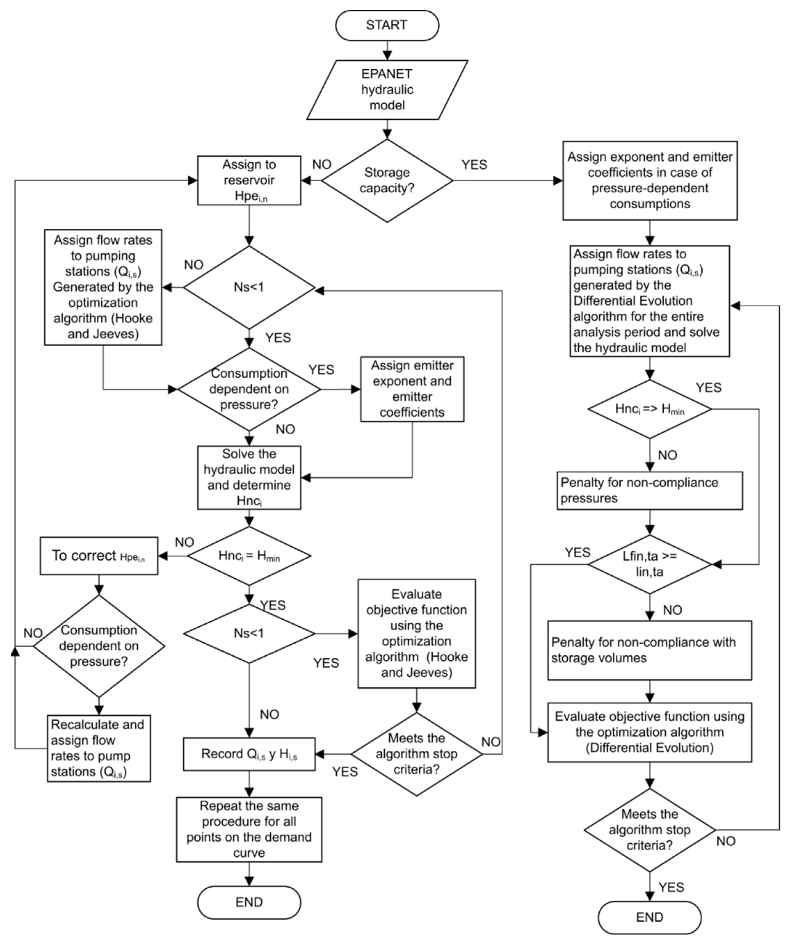
Figure 1 shows a scheme in which the process of the optimization of the setpoint curve is reflected as well as the implementation of the different algorithms.


 ,
, 


