Abstract
In recent years, due to the frequent occurrence of extreme weather due to climate change, the Taiwan region has often suffered from landslides and debris flows in the past 20 years. This study used the ground surface vibration signals collected by the geophone from seven debris flow events in the Shenmu area. Data were processed to represent the time series of velocity and accumulated energy per second. Datasets were established for model training and validation. In this study, Support Vector Machine (SVM) and Random Forest (RF) algorithms were used for comparison. After analyzing the data through balance processing (Synthetic Minority Oversampling Technique, SMOTE), a signal model of debris flow was established. The research results showed that the models using SVM and RF training had good accuracy, recall, and AUC values when choosing input data average of every 6 s and the 10-s time interval within which the data were marked as the occurrence of debris flow. The performance of SVM was better than that of RF after validation. Through the aforementioned research, the vibration signals of debris flow can be regarded as a reference factor, and the model established by the SVM method had acceptable performance and can be used for early-warning of debris flow.
1. Introduction
Taiwan is an island located in the hot zone of the Circum-Pacific Earthquake Belt, typhoons, and subtropics monsoon climatic region. Among the natural hazards, the slope-related hazards, landslides and debris flows, are the two most serious disasters to people in Taiwan [1]. The term of “debris flow” usually refers to a “very rapid to extremely rapid flow of saturated non-plastic debris in a steep channel [2,3]. By the definition, a debris flow usually occurs as the complex mixture of abundant water and sediment that may come from the channel slopes or the erosion of the beds. In addition to the non-plastic or non-Newtonian flow behavior, the typical features of debris flows are a steep boulder front-end, inverse grading of the deposit, a lateral leveed path, high flow velocity, and a peak discharge that can greatly exceed the peak discharge of debris floods or hyperconcentrated flows [4,5,6,7].
The mechanism of debris flow is a major research topic, including the initiation and movement of debris flows. The initiation of debris flows usually occurs by several mechanism, such as landslides, dam collapse, and bed erosion in the steep slope [8]. The study of debris-flow mechanism contains the effects of hydrodynamic force, the sediment concentration, and the ratio of fine-to-coarse sediments [8,9,10,11]. The effects of runoff in a steep stream are also discussed and considered in the triggering mechanism [6,12].
Among the previous studies about debris flows, the features or factors used in either the numerical model or the practical relationships, rely on the available monitoring data that are measured on-site or in the labs. The intention of these studies is mainly to find out the pattern that can be applied for debris-flow prediction or debris-flow warning. Regardless of research or warning intentions, many monitoring systems have been established worldwide, and the number of existing sites has grown significantly in the last 20 years [7]. The instruments commonly used for a debris-flow monitoring system are the sensors to measure the rainfall, soil moisture, and flow speed [1,7,13].
Similar to these debris-flow monitoring systems, the monitoring systems of lahar have been established at many volcanoes around the world, like the examples from Indonesia [14]. Some available debris-flow monitoring techniques, like those associated with the ground surface vibration-signal detectors, came from the lahar monitoring systems on volcanoes [15,16,17,18]. Itakura et al. [19] presented a list of about 70 research papers related to debris-flow monitoring, providing study sources related to warning, prediction, and modelling. The application of ground surface vibration signals in Taiwan’s debris-flow monitoring system is the focus of this study.
To protect people from the impacts of debris flows, Taiwan government, Soil and Water Conservation Bureau (SWCB), started to build debris- flow monitoring stations and a warning system since 2002. Currently there are 19 debris-flow monitoring stations in Taiwan. Most of the stations are located in central Taiwan.
The warning system developed by SWCB for debris-flow disasters was primarily based on the estimation and prediction of rainfalls. The warning model was derived from research in which the rainfall was widely used as the major triggering factor for debris flows [20,21]. The measurement of rainfall, however, is an indirect measurement of debris flows [13]. The rainfall warning is useful for disaster response but usually results in “false alarms”. A recent review [7] discusses the achievements and open problems in debris-flow monitoring. The monitoring site conditions, local features of Shenmu area, and debris flow events were used as an important monitoring case in many studies [1,7,13,22].
Instead of the rainfall factors used in the previous studies, the analysis of ground surface vibration generated during a debris flow is the main purpose of this study. Artificial intelligence has become a popular data analysis method in recent years [23] utilizing machine learning, and deep learning algorithms have become more efficient and reliable in recent years. The machine learning algorithm, Supporting Vector Machine (SVM) and Random Forest (RF), was often used for landslide-related hazards, including debris flows, and are the study focus of this paper.
Finally, the performance of the proposed SVM and RF model was evaluated, and two events of heavy rainfalls in the case history of debris flow in the Shenmu area were used for external performance tests. The insights from the newly developed SVM model were also included in this paper.
2. Study Area and Database
The study area is at the Shemu area and there are three highly potential debris-flow torrents in this region. The three debris-flow torrents, Aiyuzi Stream, Huosa Stream, and Chusuei Stream, merge together around the village and the entire drainage area covers about 72.2 km2 [1,7]. These streams belong to the watershed of Chen-Yu-Lan River in the central part of Taiwan. The terrain and landslide areas of streams and the basic information are shown in Figure 1 and Table 1, respectively. In the study area, the debris flows commonly occurs at the Aiyuzi Stream due to its shorter length and larger landslide areas located in its upstream since Typhoon Morakot in 2009.
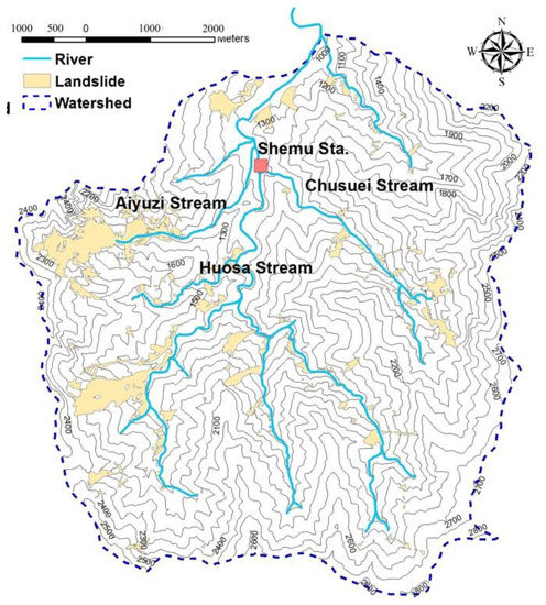
Figure 1.
The terrain and landslide areas (after 2009) of the study area in Shemu [24].

Table 1.
The landslide area in Shenmu after 2009 [1].
Aiyuzi Stream is the wild stream in the upper stream of the Chen-Yu-Lan River catchment area. The stream is labelled as DF226 and with a rainfall warning value of 250 mm for debris-flow hazards. The topographical elevation is between 1200–2500 m, and the average slope of the catchment area is about 39.3°, of which the slope greater than 55% is more than 75% of the total catchment area [25]. According to Chen [26], the landslide ratio (landslide projected area/total catchment area) of this catchment area is about 12~34.2% (1996–2009), and there is a trend of increasing year by year.
Referring to the rainfall data (from June 1987 to February 2017) of Shenmu Village Station of the Taiwan’s Central Weather Bureau (CWB), the average annual rainfall in this catchment area is about 3054.7 mm, of which the average total accumulated rainfall in the rainy season (from April to October each year) is 2644.5 mm [22]. Because of the rainfall and abundant landslide-induced soil and rock debris at the upstreams, debris flows often occurred in the Aiyuzi Stream during heavy rains and typhoons.
A debris flow monitoring station was built in 2002 in the Shenmu area (Figure 2), and the monitoring station includes different sensors to collect data principally focusing on debris-flow warning. The major sensors and devices installed in the Shenmu Monitoring Station are rain gauges and geophone, as shown in Figure 2. The measurement of rainfall is usually used for early warning of debris flows in Taiwan. The data obtained by the geophone are the ground surface vibration signals and the variation of the signals can directly indicate the occurrence of debris flows. The specification of the geophone installed in the Shenmu area is listed in Table 2.
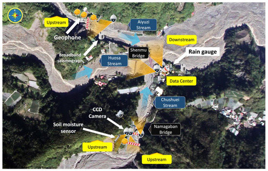
Figure 2.
The layout of monitoring devices in the Shenmu area.
Table 2.
Specification of geophone OYO Geospace GS-20DX [22].
The recorded debris flow events are summarized in Table 3. Among these events, the vibration signals from geophones are available only for several events. Seven events of 0713 Rainfall and 1110 Rainfall in 2011, 0504 Rainfall and 0610 Rainfall in 2012, 0517 Rainfall and 0713 Rainfall (Typhoon Saulik) in 2013, and 0520 Rainfall in 2014 were used in this study. Data from the first five of seven events were used for model training and the other two events were used for external validation of model performance. Figure 3, Figure 4, Figure 5 and Figure 6 show the plots of vibration signals in terms of time series of velocity and accumulated energy per second.
Table 3.
Debris flow hazard history of Shenmu [24].
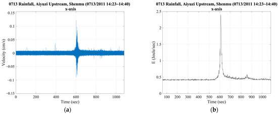
Figure 3.
The data of 0713 Rainfall in 2011 (a) vibration signals (b) accumulated energy per second.
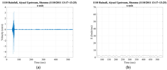
Figure 4.
The data of 1110 Rainfall in 2011 (a) vibration signals (b) accumulated energy per second.
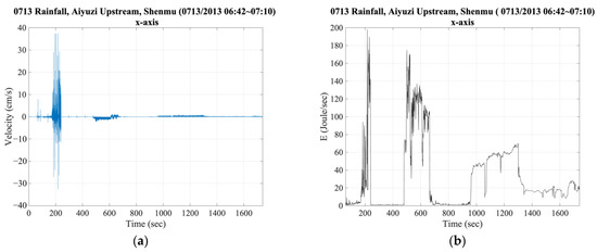
Figure 5.
The data of Typhoon Saulik (0713) Rainfall in 2013 (a) vibration signals (b) accumulated energy per second.
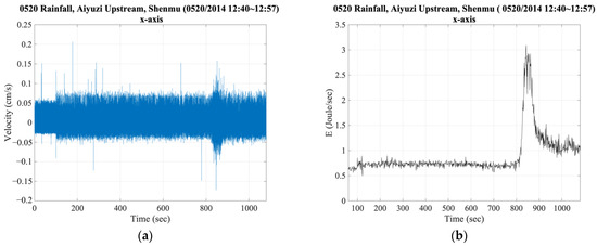
Figure 6.
The data of 0520 Rainfall in 2014 (a) vibration signals (b) accumulated energy per second.
3. Evaluation Methods
To set up the evaluation model using vibration signals of debris flows, the major work was to determine the factors that could describe the vibration-signal patterns of debris flows. The pattern in this study was defined as the periods of pre- and post-debris flow, especially the background vibration signals during the non-event time, and the period that the debris flow passed through the locations of geophones. Therefore, the timing of broken wire-sensors was used as reference to determine the time intervals used for pattern evaluation. From the plots of signals, it had been found that the arrival of debris flows usually had peaks in the recorded vibration signals.
Previous studies suggested that the original geophone signals, in terms of velocity (cm/s), and the correspondingly estimated accumulated energy, in the unit of joule (J), of the three axes, x, y, and z, were the major factors used for vibration-signal analysis [1,24]. This study used the recorded signals and processed the velocity data recorded by the geophones to obtain the corresponding accumulated energy values. The factor of accumulated energy per second was used in the study. The signals form all three axes were processed in the same way before constructing the training and validating datasets. Figure 3 shows an example of time series plots of original signals and the accumulated energy per second.
The datasets were built by first averaging the 500 data entries per second (250-Hz sampling rate) of three axes for each event, to obtain the velocity time series in seconds, which were defined as velocity factors of Vx, Vy, and Vz. Then the accumulated energy per second, defined as energy factors of Ex, Ey, and Ez, was estimated accordingly by the converting process. There were two datasets of vibration signals used in this study. One was the training dataset (from the first five debris flow events) and the other was the validation dataset (from the other two debris flow events).
In combination with the velocity and energy factors, the patterns of signals were defined as shown in Figure 7, by labeling data as 0 and 1, representing the periods of pre- and post-debris flow, and the occurrence of debris flow, respectively. For a given debris-flow vibration signal plot, the peak value was the reference point to divide the time series of data into sections. The selection of time interval of Label-1 was evaluated and determined by assuming different periods of 10, 20, 30, and 45 s. The trials of these time intervals were conducted in the models by using machine learning methods. As an example, Table 4 shows the number of samples of Label-0 and Label-1 based on the 45-s time interval of each event.
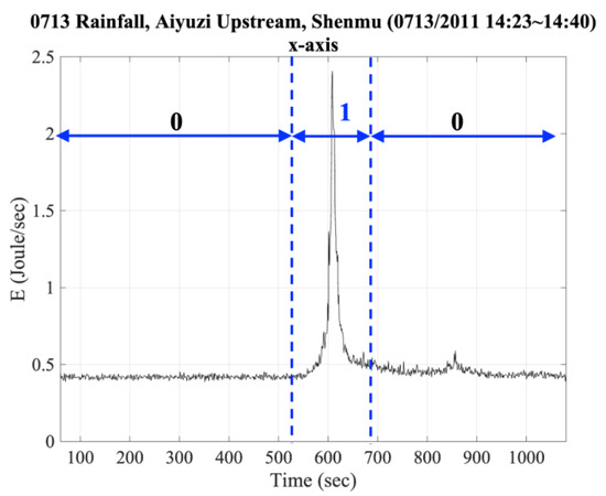
Figure 7.
The illustration of labeling of debris-flow vibration signals.
Table 4.
Sample numbers of 45-s interval trial.
The factors used for selection were velocity factors, Vx, Vy, and Vz, and the accumulated energy per second, Ex, Ey, and Ez, of three axes. With these factors, the analysis of this study conducted in two stages. Stage one focused on the factor selection to use fewer factors in the modeling. Next stage was set to test the performance of models by applying different combinations of time series and time intervals of labeling. For time series, the trial dataset was constructed by picking up the entry from every second to every 10 s. For labeling intervals, as mentioned previously, four intervals of 10, 20, 30, and 45 s, were used in the testing. The confusion matrix of the model (Table 5) was used to evaluate the outcomes of each trial.
Table 5.
The confusion matrix of debris-flow occurrence based on the vibration signal labeling.
Based on the confusion matrix, the indices of accuracy (ACC), sensitivity or recall, precision, area under the ROC curve (AUC), and Kappa (kappa index of agreement, KIA) were used to validate the performance of each trial combination. Because of the imbalanced original data of Label-0 and Lable-1, the result of only using the index of accuracy had tended to over-fit the classification of no debris flow, because there were more Lable-0 data than Label-1 data. Instead, the index of Kappa was more reliable when evaluating the model performance since its value represented the bias of conditions if any. Therefore, both indices of accuracy and Kappa were used for evaluation, and the Kappa was the key factor for final decision. A Kappa value greater than 0.75 is considered as good precision [27].
The algorithm of SVM and RF were adopted for model training and validation, and the program WEKA [28] was used in this study. The synthetic minority oversampling technique (SMOTE) was also applied to ease the impact of imbalanced dataset.
4. Results and Discussion
Based on the factor combinations mentioned in the previous section, there were total of 482 trail models generated during the first stage. In this stage, both algorithm of SVM and RF were used with the same data ratio of training to self-validation, i.e., 7:3, and the gain ratios from WEKA were obtained to determine the importance ranking of factors. The close the gain ratio is to 1, the greater the influence. After performing SVM and RF on all combinations of factors, Figure 8 shows the sum of gain ratios, and it was noted that the top three important factors were the accumulated energy per second of the axes. Thus, the accumulated energy per second was used as the main factor in the following model setup and evaluation.
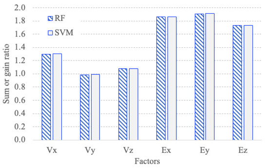
Figure 8.
The factor ranking based on the gain rations.
The next stage of modeling was to evaluate the performance of combinations from the choices of input data from the average every second to the average every 10 s, and the time intervals of Label-1, i.e., 10, 20, 30, and 45 s. Both SVM and RF were applied again and the three indicis of accuracy, recall, and Kappa were used to represent the ranking order of each choice. Figure 9, Figure 10 and Figure 11 show the results of input-data average from every second to every 10 s, and it was noted that input-data average of every 6 s was the best performance from all three indices. For time intervals of Label-1, Figure 12 shows the results of accuracy index, implying that the best performance was achieved by using the time interval of 10 s.
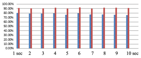
Figure 9.
The accuracy values of input data average (blue bars for SVM and red bars for RF).
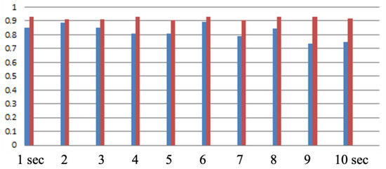
Figure 10.
The recall values of input data average (blue bars for SVM and red bars for RF).
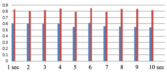
Figure 11.
The Kappa values of input data average (blue bars for SVM and red bars for RF).
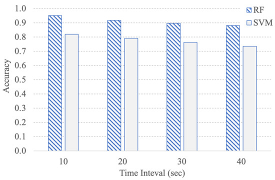
Figure 12.
The accuracy values of time intervals.
After the two-stage testing, the final model was established by choosing the input-data average of every 6 s, and the time interval of 10 s as the Label-1 data. The data from five events of 0713 Rainfall and 1110 Rainfall in 2011, 0504 Rainfall and 0610 Rainfall in 2012, and 0517 Rainfall in 2013, were used for model training and self-validation. Then, the cases of 0713 Rainfall (Typhoon Saulik) in 2013 and the 0520 Rainfall in 2014 were used for additional performance validation. Table 6 shows the results of performance validation.
Table 6.
External validation results.
According to the results of external verification, both two algorithms had high accuracy, very good recall values and high AUC, indicating the low missing rate of the model. From the precision index, however, SVM model performed much better than RF model, implying that SVM model had much lower rate of misjudgment. Also, higher Kappa value of SVM indicated that the SVM model was more suitable than the RF model. From the abovementioned five indices, the SVM model was more reliable than the RF model in terms of capturing the vibration-signal patter of debris flows.
5. Conclusions
With the evaluation of the vibration signals of several debris flows in the Shenmu area, the analysis led to the following conclusions.
The purpose of this research is to investigate whether the signal data obtained from the geophones can be used to determine the occurrence of events through the classification algorithm SVM and RF. The results shows that the performance of the proposed model was considerably acceptable, and the vibration signal is potentially practical for debris flow prediction and warning
- The factors that affected the model performance were compared and it was found that the energy factor, the accumulated energy per second of the X, Y, and Z axes, was the most important and influential factor in the model. The test of data selection also implied that the every-6-s average value of the accumulated energy per second, and the Lable-1 data of 10-s interval before and after the peak signals had better performance in capturing the debris-flow vibration-signal pattern. Therefore, the data preparation using 6-s average of accumulated energy per second and 10-s interval for labeling debris-flow occurrence were considered suitable for model training.
- The performance validation using two cases had shown that both the SVM and RF models had high accuracy greater than 0.9, but the precision and Kappa values implied that the SVM model was better than the RF model. Therefore, the proposed SVM model, with the data selection method addressed in this study, was considered applicable in predicting the debris flow in the study area. Based on the analysis results, the procedure of setting up machine learning model in this study can be extended to the practical level for debris-flow disaster management.
Author Contributions
Conceptualization, Y.-M.H.; methodology, Y.-M.H.; software, C.-C.C.; validation, Y.-M.H. and C.-C.C.; formal analysis, Y.-M.H. and C.-C.C.; investigation, Y.-M.H.; resources, Y.-M.H.; data curation, Y.-M.H. and C.-C.C.; writing—original draft preparation, Y.-M.H.; writing—review and editing, Y.-M.H.; visualization, Y.-M.H. and C.-C.C.; supervision, Y.-M.H.; project administration, Y.-M.H.; funding acquisition, Y.-M.H. All authors have read and agreed to the published version of the manuscript.
Funding
This research was funded by Soil and Water Conservation Bureau, Council of Agriculture, Executive Yuan, Taiwan, grant number SWCB-1110111015A.
Institutional Review Board Statement
Not applicable.
Informed Consent Statement
Not applicable.
Data Availability Statement
No new data were created or analyzed in this study. Data sharing is not applicable to this article.
Acknowledgments
Authors would like to thank the editor and anonymous reviewers for the careful review of the original manuscript.
Conflicts of Interest
The authors declare no conflict of interest. The funders had no role in the design of the study; in the collection, analyses, or interpretation of data; in the writing of the manuscript, or in the decision to publish the results.
References
- Huang, Y.M.; Chu, C.R.; Fang, Y.M.; Tsai, M.C.; Lee, B.J.; Chou, T.Y.; Lee, C.Y.; Chen, C.Y.; Yin, H.Y. Characteristics of debris flow vibration signals in Shenmu, Taiwan. In Proceedings of the Interpraevent International Symposium, Lucerne, Switzerland, 30 May–2 June 2016; 2016. Available online: https://interpraevent2016.ch/ (accessed on 28 September 2022).
- Hungr, O.; Evans, S.G.; Bovis, M.J.; Hutchinson, J.N. A review of the classification of landslides of the flow type. Environ. Eng. Geosci. 2001, 7, 221–238. [Google Scholar] [CrossRef]
- Hungr, O.; Leroueil, S.; Picarelli, L. The Varnes classification of landslide types, an update. Landslides 2014, 11, 167–194. [Google Scholar] [CrossRef]
- Iverson, R.M. The physics of debris flows. Rev. Geophys. 1997, 35, 245–296. [Google Scholar] [CrossRef]
- Jakob, M.; Hungr, O. Debris-Flow Hazards and Related Phenomena; Springer: Berlin/Heidelberg, Germany, 2005; p. 739. [Google Scholar]
- Takahashi, T. Debris Flow: Mechanics, Prediction and Countermeasures, 2nd ed.; CRC Press/Balkema: Boca Raton, FL, USA, 2019. [Google Scholar]
- Hürlimann, M.; Coviello, V.; Bel, C.; Guo, X.; Berti, M.; Graf, C.; Hübl, J.; Miyata, S.; Smith, J.B.; Yin, H.-Y. Debris-flow monitoring and warning: Review and examples. Earth-Sci. Rev. 2019, 199, 52. [Google Scholar] [CrossRef]
- Hairani, A.; Rahardjo, A.P. A Theoretical Model for Debris Flow Initiation by Considering Effect of Hydrodynamic Force. In Proceedings of the 4th International Conference on Sustainable Innovation 2020–Technology, Engineering and Agriculture (ICoSITEA 2020), Yogyakarta, Indonesia, 13–14 October 2021; Atlantis Press: Dordrecht, The Netherlands; pp. 38–42. [Google Scholar] [CrossRef]
- Guo, C.X.; Zhou, J.W.; Cui, P.; Hao, M.H.; Xu, F.G. A theoretical model for the initiation of debris flow in unconsolidated soil under hydrodynamic conditions. Nat. Hazards Earth Syst. Sci. Discuss 2014, 2, 4487–4524. [Google Scholar]
- Schippa, L. Modeling the effect of sediment concentration on the flow–like behaviour of natural debris flow. Int. J. Sediment Res. 2020, 35, 315–327. [Google Scholar] [CrossRef]
- Schippa, L. Yield Stress Model for Natural Debris Flows in Presence of Fine and Coarse–Grained Sediments. Water 2021, 13, 1865. [Google Scholar] [CrossRef]
- Mukhlisin, M.; Kosugi, K.; Mizuyama, T. Temporal and spatial variations in the probability of debris flow initiation in volcanic watersheds. J. Jpn. Soc. Eros. Control. Eng. 2005, 57, 3–14. [Google Scholar]
- Huang, Y.M.; Chen, W.C.; Fang, Y.M.; Lee, B.J.; Chou, T.Y.; Yin, H.Y. Debris Flow Monitoring—A Case Study of Shenmu Area in Taiwan. Disaster Adv. 2013, 6, 1–9. [Google Scholar]
- Lavigne, F.; Thouret, J.C.; Voight, B.; Young, K.; LaHusen, R.; Marso, J.; Suwa, H.; Sumaryono, A.; Sayudi, D.S.; Dejean, M. Instrumental lahar monitoring at Merapi Volcano, Central Java, Indonesia. J. Volcanol. Geotherm. Res. 2000, 100, 457–478. [Google Scholar] [CrossRef]
- Bautista, B.C.; Bautista, M.L.P.; Garcia, D.C. Seismic monitoring: A useful tool for mudflow detection at Mayon volcano, Albay, Philippines. Philipp. J. Volcanol. 1986, 3, 90–108. [Google Scholar]
- Marcial, S.; Melosantos, A.A.; Hadley, K.C.; LaHusen, R.G.; Marso, J.N. Instrumental lahar monitoring at Mount Pinatubo. In Fire and Mud: Eruptions and Lahars of Mount Pinatubo, Philippines; Newhall, C.G., Punongbayan, R.S., Eds.; Washington Press: Seattle, WA, USA, 1996; pp. 1015–1022. [Google Scholar]
- Suwa, H.; Okano, K.; Kanno, T. Forty years of debris-flow monitoring at Kamikamihorizawa Creek, Mount Yakedake. Ital. J. Eng. Geol. Environ. Nov. 2011, 605–613. [Google Scholar] [CrossRef]
- Itakura, Y.; Fujii, N.; Sawada, T. Basic characteristics of ground vibration sensors for the detection of debris flow. Phys. Chem. Earth Part B 2000, 25, 717–720. [Google Scholar] [CrossRef]
- Itakura, Y.; Inaba, H.; Sawada, T. A debris-flow monitoring devices and methods bibliography. Nat. Hazards Earth Syst. Sci. 2005, 5, 971–977. [Google Scholar] [CrossRef]
- Jan, C.D.; Lee, M.H.; Huang, T.H. Effect of Rainfall on Debris Flows in Taiwan. In Proceedings of the International Conference on Slope Engineering, Hong Kong, China, 8–10 December 2003; Volume 2, pp. 741–751. [Google Scholar]
- Jan, C.D.; Lee, M.H. A Debris-Flow Rainfall-Based Warning Model. J. Chin. Soil Water Conserv. 2004, 35, 275–285. [Google Scholar]
- Wei, S.C.; Liu, K.F.; Huang, Y.M.; Fang, Y.M.; Yin, H.Y.; Huang, H.Y.; Lin, C.L. Characteristics and Warning Methods of Ground Vibrations Generated by Debris Flows at Ai-Yu-Zi Creek. J. Chin. Soil Water Conserv. 2018, 49, 77–88. [Google Scholar] [CrossRef]
- Tan, L.; Guo, J.; Mohanarajah, S.; Zhou, K. Can we detect trends in natural disaster management with artificial intelligence? A review of modeling practices. Nat. Hazards 2021, 107, 2389–2417. [Google Scholar] [CrossRef]
- Huang, Y.M.; Fang, Y.M.; Yin, H.Y. The Vibrational Characteristics of Debris Flow in Taiwan. In Proceedings of the 7th International Conference on Debris-Flow Hazard Mitigation, Golden, CO, USA, 10–13 June 2019; p. 8. [Google Scholar] [CrossRef]
- Huang, C.J.; Yin, H.Y.; Chen, C.Y.; Yeh, C.H.; Wang, C.H. Ground vibrations produced by rock motions and debris flows. J. Geophys. Res. 2007, 112, F02014. [Google Scholar] [CrossRef]
- Chen, S.C.; Chen, S.C.; Wu, C.H. Characteristics of the landslides in Shenmu watershed in Nantou County. J. Chin. Soil Water Conserv. 2012, 43, 214–226. [Google Scholar] [CrossRef]
- Fleiss, J.L.; Levin, B.; Paik, M.C. Statistical Methods for Rates and Proportions, 3rd ed.; Wiley-Interscience: Hoboken, NJ, USA, 2003. [Google Scholar]
- Eibe, F.; Hall, M.A.; Witten, I.H. The WEKA Workbench. Online Appendix for Data Mining: Practical Machine Learning Tools and Techniques, 4th ed.; Morgan Kaufmann: San Francisco, CA, USA, 2016. [Google Scholar]


Publisher’s Note: MDPI stays neutral with regard to jurisdictional claims in published maps and institutional affiliations. |
© 2022 by the authors. Licensee MDPI, Basel, Switzerland. This article is an open access article distributed under the terms and conditions of the Creative Commons Attribution (CC BY) license (https://creativecommons.org/licenses/by/4.0/).