Abstract
Hydraulic models of rivers are essential for vulnerability assessment in disaster management. This study simulates the 2019 Typhoon Hagibis at the Nanakita River using a dynamic roughness model. The model estimates the roughness of the river on a pixel level from the relationship between the Manning roughness coefficient and the degree of submergence of vegetation. This degree is defined as the ratio of water depth to plant height. After validating the model, the effect of vegetation on the water level in different seasons from April 2020 to March 2021 was assessed. The vegetation area and height were obtained on a pixel level using unmanned aerial vehicle photogrammetry. The dynamic roughness model showed that the water level profile increased by 7.03% on average. The seasonal effect of vegetation was observed, revealing a strong correlation between variations in the vegetation conditions and water level profile. This approach may help mitigate flood damage by indicating the factors that can increase the risk of flooding.
1. Introduction
Hydraulic models of rivers are essential for vulnerability assessment in disaster management, especially in areas prone to floods due to cyclones and typhoons. These models are influenced by various parameters, with roughness as the most critical. Roughness has several influencing factors [1], with vegetation as the dominant [2]. Several investigations on the effect of vegetation on flow and roughness have been made [2,3,4,5,6,7,8,9,10,11,12]. Studies have attributed the roughness variation to the degree of submergence of plants [2,5,6,7,8] and plant density [2,9,10,11]. It is important to note that other factors such as the plant morphology and flexibility play an important role in the roughness determination [12]. Physical parameters are the primary determinants of roughness, and the ratio of the average canopy height to the mean flow depth is the most accurate descriptor of roughness [5]; consequently, with depth fluctuations in flood events, the roughness value is a dynamic variable. Hence, constant roughness is not applicable for every type of flow condition [2]. Mohammadi and Kashefipour [13] considered the flow depth and velocity as variables to calculate a dynamic roughness value in the Kārūn River, Iran, without directly considering the vegetation. Yoshida et al. [14] used vegetation information acquired by LiDAR to calculate a distributed roughness based on the vegetative drag force dynamically in a flood model. Variations of vegetation characteristics due to seasonal change alter the flow dynamics of rivers [15], making vegetation control at the riverbank a crucial task.
Vegetation characteristics are often excluded from hydraulic modeling due to high time consumption and financial cost. Unmanned aerial vehicles (UAVs) are useful tools for acquiring the data through river mapping [14,16,17,18,19]. Combining high-resolution UAV imagery with artificial neural networks (ANN) is a good strategy to identify vegetation and other features in river environments [17]. In addition, UAV imagery has enabled the creation of three-dimensional (3D) terrain models through structure from the motion (SfM) approach [18], being used to monitor seasonal variations of riparian vegetation height [19]. UAVs with real-time kinematic (RTK) positioning have obviated the need for ground control points to generate accurate digital surface models (DSMs) from 3D point clouds, improving the photogrammetry process. This has further reduced the computational cost and time required to generate 3D point clouds accurate to less than 10 cm [20]. Studies that consider the vegetation-induced roughness in hydraulic modeling from remote-sensed vegetation data, especially height and density, are needed [21]. Furthermore, the pixel-based acquisition of vegetation information through UAV imagery has allowed the application of dynamic vegetative roughness estimation for flood analysis. In addition, affordable UAV imagery and photogrammetry with RTK positioning allow frequent observations and acquisitions of seasonal vegetation information.
With many rivers, Japan is often affected by typhoons and suffers constant river flooding. Yet, the country has not implemented sufficient vegetation management to mitigate typhoon induced inundations. About 90% of Japan’s river length is administered by prefectural governments, of which only a few rivers are overseen by management strategies owing to budgetary constraints. On 12 October 2019, Typhoon Hagibis devastated ten prefectures in Japan with record rainfall and wind speeds [22]. According to the Ministry of Land, Infrastructure, Transport and Tourism [23], the event overtopped approximately 130 embankments along several rivers, causing 90 deaths and nine disappearances and damaging approximately 80,000 houses. In Miyagi prefecture, the floods severely damaged the town of Marumori and abutting areas [24]. To ensure the safety of the population, flood vulnerability studies are very important for indicating factors that can increase the flood risk at determined locations [25]. This is mostly important for small- and medium-sized rivers because they tend to flood more severely than large rivers.
The objectives of this study are (1) to estimate the seasonal effect of the riparian vegetation on flow dynamics using a dynamic roughness hydraulic model, (2) to obtain the vegetation conditions throughout the year from 3D point cloud data, (3) to quantify the effect of riparian vegetation on flood vulnerability through a case study of Typhoon Hagibis, and (4) to assess the effect of the seasonal variation of vegetation conditions on the changes in water level using the hydraulic event of Typhoon Hagibis.
2. Study Area
The rivers in Japan are classified into Class A and Class B depending on their dimension as well as their social importance [26]. Class A rivers are managed by the national government, whereas Class B rivers are managed by the prefectural governments. Nanakita River is a Class B river located in Miyagi prefecture; it courses through the cities of Sendai and Tagajo. According to Viet et al. [27], the river has a length of 45 km and a catchment area of 229 km2, the average annual discharge is 10 m3/s, and the flood discharge of a 100-year return period is 1650 m3/s. The bed slope of the Nanakita River is about 0.0016 in the relatively upstream reach and about 0.0003 in the lower reach [28].
The effect of vegetation on the flow dynamics is more visible in Class B rivers owing to their smaller size, and therefore, the Nanakita River is suitable for achieving the research objectives of this study. The Nanakita Dam was constructed in the upstream part of the river basin. According to the Japan Dam Foundation [29], the dam type is a rockfill dam; it has a water surface area of 50 hectares and a capacity of 9,200,000 m3, with the purpose of flood control, river flow maintenance, and water supply. According to the prefecture’s administration, the dam was not assigned the control of the river discharge at the time of Typhoon Hagibis.
The Nanakita River is the only Class B river in the prefecture with a flood forecast system, which is effective in the downstream portion of the river. The upstream region relies on a water level awareness system. The river catchment is a flood-prone area and the river has overflowed several times in the past due to heavy rains. The last flood occurred in 2015 caused by typhoons 17 and 18 [30].
Figure 1a–c show a map of the Nanakita River basin location in Miyagi prefecture, its topography and river system with the location of the dam and five water level gauge stations, and the 2 km stretch of the river chosen for the two-dimensional (2D) hydraulic simulation, respectively. This stretch has a dense population and is frequented by residents, with many houses on the coast. It is densely vegetated, with a predominant population of Pueraria montana var. Lobata (Kudzu), Miscanthus sinensis, Phragmites australis, and Solidago canadensis, making it ideal for studying the effects of a typhoon. In addition, although the water level reached a considerable height, no overtopping of the embankments happened during the typhoon event.
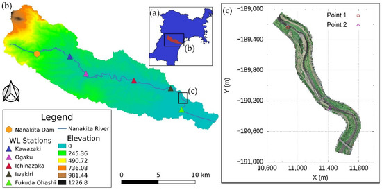
Figure 1.
Study area: (a) Location of the Nanakita River basin in Miyagi prefecture; (b) basin map with the topography used as calculation area for the rainfall-runoff inundation model; (c) the 2 km stretch of the Nanakita River obtained from the UAV observation of September 2019 used as calculation area for the 2D hydraulic model.
Thirteen UAV observations took place in the stretch shown in Figure 1c, once in September 2019 and then monthly from April 2020 to March 2021. The prefecture removed the vegetation in October 2019, right after the disaster, as a countermeasure but could not continue the efforts owing to regrowth.
3. Methodology
The 2019 Typhoon Hagibis was simulated with a 2D hydraulic model in the UAV observed area shown in Figure 1c; the model was altered to dynamically calculate the Manning roughness coefficient considering the vegetation height (dynamic roughness model). The discharge of the event in the upstream section of the stretch was first generated by the rainfall–runoff–inundation (RRI) model.
The vegetation conditions in September 2019 and from April 2020 to March 2021 were obtained from the 3D point cloud data files.
The recreation of Typhoon Hagibis using the dynamic roughness model used the vegetation conditions obtained from the September 2019 UAV observation, which contained the pre-event conditions. The results of the simulation were compared with those of a static roughness simulation (2D hydraulic model before the alteration). Both simulations used the same topography and discharge, the only difference being the roughness setting; whereas the dynamic model calculated the Manning roughness coefficient for the entire simulation period, the static model considered it a constant value.
After model validation, the seasonal effect of the vegetation on the water level of the river was assessed. To this end, the same hydrologic event was simulated 12 more times, wherein only the vegetation conditions obtained from the monthly UAV observations from April 2020 to March 2021 were varied.
3.1. UAV Observations
The purpose of UAV photogrammetry was to obtain the vegetation information and determine the seasonal changes of the riparian vegetation on the river floodplains. We captured photographs once in September 2019 and then monthly from April 2020 to March 2021. Thus, we generated 13 orthophotographs and 3D point cloud data files. The UAV (Phantom 4RTK (DJI)) has an RTK module that receives data from satellites and fixed bases and accurately corrects the position of the image in flight in real time. The observations were shot from an altitude of 50 m. The wrap rate was set at 80% overlap and 60% side wrap. To improve the accuracy of the images in the vertical direction, a camera inclined at 70° was mounted for the SfM analysis.
The point cloud had a vertical accuracy of less than 10 cm at the top of the embankment (approximately 8 cm).
Metashape (Agisoft) was used for the SfM analysis, and the point cloud density was 400 points m–2.
3.2. Hydrologic Model
The RRI model was used for the hydrologic simulation; it is a 2D model that can simulate both rainfall–runoff and inundation [31,32,33,34]. The model used the following input data: (1) the observed rainfall data collected from radar/rain gauge-analyzed (RA) precipitation [35] with hourly observations spanning 48 h from October 12 to 14, 2019; (2) the MERIT hydro digital elevation model (DEM) [36] with a resolution of 90 m used for the topographic data; and (3) the land-cover map from the MLITT [23] with a resolution of 100 m. In this model, a Manning roughness coefficient value of 0.04 was adopted for the river channel. In the slope area, the values were 0.5, 0.3, and 0.04 for vegetated areas, urban areas, and water bodies, respectively. The soil depth of the vegetated area was assumed to be 1.0 m, whereas that of the other two areas were assumed to be 0.1 m. Simulated and observed water depth in the five water level gauge stations shown in Figure 1b were used to validate the model.
3.3. Two-Dimensional Hydraulic Model
The 2D hydraulic model used for flood inundation was developed by Iwasa and Inoue [37] and Inoue et al. [38], and further used in Hashimoto et al. [39]. The model utilizes the continuity and momentum equations in the x- and y-directions as governing equations, shown in Equations (1)–(3).
where h is the depth, x and y are the flux directions, and u and v are the flow velocities in the x and y directions, respectively. M = u × h, N = v × h, n is the roughness factor, and H is the water level.
The topographic data for the model was constructed by interpolating the 21 cross-sections spaced 100 m apart provided by the Miyagi prefecture administration. Thus, a DEM with 23,040 cells with 10 m resolution was generated. The 10 m grid cell was chosen because it accurately represents the vegetation in the UAV-observed area. The hydraulic data used as input was the discharge obtained from RRI model.
3.4. Dynamic Roughness
The hydraulic model was patched with a pixel-based dynamic-roughness calculation routine based on the degree of submergence of vegetation. The concept of the degree of submergence is illustrated in Figure 2, as described in Nikora et al. [5], and is defined by the ratio of the water depth to the vegetation height (Equation (4)).
where hwater is the water depth of the section, and hvegetation is the vegetation height.
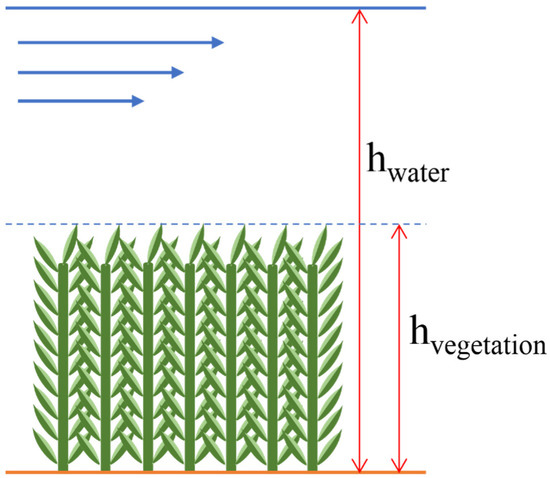
Figure 2.
Scheme showing the degree of submergence of the vegetation.
The code adaptation comprehends the creation of a new input file with the location of the grid cells with vegetation and the vegetation height in each cell. The model then calculates the pixel-based roughness at every vegetated grid cell for each loop of the simulation, based on the degree of submergence of vegetation using the formula presented in Equation (5), obtained from the analysis of the relationship between the two parameters by the Japan Institute of Country-ology and Engineering [40]. The data present in [40] was obtained by field experiment, and the equation was obtained from regression analysis using MATLAB. The analysis produced a coefficient of determination (R²) of 0.88 and a root mean square error (RMSE) of 0.007. Unlike the dynamic roughness calculation method of Mohammadi and Kashefipour [13], which used only water depth and velocity threshold to define roughness, this model directly correlated the hydraulic resistance with the vegetation height.
Figure 3 shows a representation of the relationship between the Manning roughness coefficient and the degree of submergence of various types of vegetation obtained from the Japan Institute of Country-ology and Engineering [40] and the regression equation. The equation from this relationship was derived from all the points shown in Figure 3, unifying all types of grass vegetation hardness into a single curve.
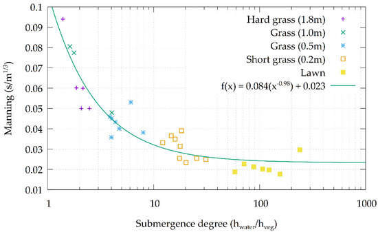
Figure 3.
Relationship between the Manning roughness coefficient and the degree of submergence for different types of vegetation hardness and the regression curve.
In the code adaptation, the estimation of the Manning roughness coefficient is only applicable for fully submerged vegetation, when the degree of submergence is higher than 1; therefore, when the vegetation is emerging (degree of submergence less than or equal to 1), the model assumes a no-flow condition, where the water enters the cell and is trapped until it submerges the vegetation. For non-vegetated grid cells, the Manning roughness coefficient was set to a constant value of 0.022, a value recommended by Arcement and Verne [41], considering the surface material to be a smooth, firm soil.
The results from the dynamic roughness model were compared with those from the static model. The latter used constant Manning roughness coefficient values of 0.022 for the channel area and 0.038 for the floodplains; the values were fixed by river management. The value for the channel was set according to the bed material, composed mainly of firm soil and sand, whereas the value for the floodplains was chosen considering the range between 0.025 and 0.050 that represents a large amount of vegetation, according to Arcement and Verne [41]. To identify channel and floodplain, a simulation in the same area was performed with the average yearly discharge of 10 m3/s. Both simulations were validated by comparing the water level profile in the peak with the floodmark points at specific locations.
3.5. Vegetation Characteristics
A Fortran 90 program was written to obtain digital surface models (DSMs) and RGB orthoimages from each of the UAV 3D point cloud data files. The RGB images were used to obtain the vegetation location with a multi-layer perceptron (MLP) algorithm trained based on the RGB values, and the DSMs were used to obtain the vegetation height for each month.
Because of the change of the vegetation color with the passing of seasons, two MLP models were trained, one for the spring and summer seasons (group 1) and another for the autumn and winter (group 2). Figure 4 depicts a flowchart with the steps for the acquisition of the vegetation location for the spring and summer seasons.
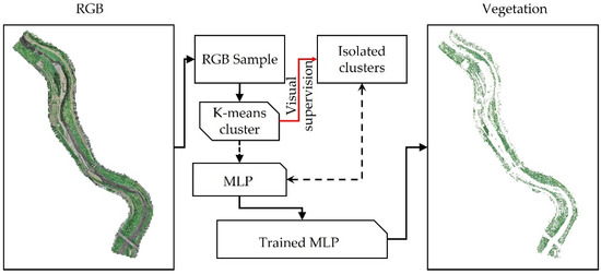
Figure 4.
Flowchart of the method for the identification of the vegetated grid cells.
The method of identification of the vegetated pixel was similar to the method applied by Casado et al. [17]: rather than identifying all the features in the river environment, this study focused only in the identification of the vegetation. First, two samples of the RGB images of September 2019 and January 2021 with resolution of 1 m were cropped and submitted to a k-means cluster algorithm. Different from Casado et al. [17], who used the CIELAB color spectrum to cluster the pixels, in this methodology, the RGB color spectrum was used. Each cluster was isolated, and visual supervision was used to obtain the vegetated pixels for the two samples. Once the vegetation was located, the MLP models were trained for each group. Subsequently, the trained models were used to predict the vegetation location in the entire RGB images. The images were re-sampled to a 10 m grid size with ArcMAP 10.5, using the Majority algorithm to match the cell size chosen for the hydraulic simulations. The Majority algorithm determined the new value of the larger cell based on the most popular values between the smaller grid cells in the location. This method produced smoother results than the nearest neighbor method, avoiding the overestimation of the vegetation conditions.
With the vegetated grid cells located, the vegetation height could be calculated. As discussed in Weidner and Förstner [42], the DSM differs from the DEM because it comprehends not only the ground level but the level of the objects above; therefore, by normalizing the DSM with the DEM, the height of the aboveground objects can be determined. Thus, the vegetation height was obtained by this method only at the vegetated grid cells. Differing from the methodology used by van Iersel et al. [19], the normalization was performed with the DEM obtained from the interpolated cross-sections rather than from a digital terrain model (DTM), which is calculated from the DSM by removing the objects above ground level. The accuracy of the DTM depends on the time when the UAV observation is performed, varying with the seasons.
4. Results and Discussion
4.1. Vegetation Conditions
Both MLP models obtained good accuracy and made good predictions of the vegetation location, like the results obtained in [17]. The model accuracy for group 1 was 0.99. Group 2 obtained an accuracy of 0.96, as shown in Table 1, along with other evaluation parameters.

Table 1.
Evaluation parameters of the MLP model of both groups.
The precision and accuracy achieved for group 2 was considerably lower than the accuracy of group 1. The same can be observed for the precision; thus, the MLP trained for group 1 was able to classify the pixels with more correction than group 2. In addition, misclassification of group 2 was higher, meaning that more non-vegetated pixels were wrongfully classified as vegetated pixels in group 2 than in group 1, although, with the misclassification value of 4%, the wrongfully classified pixels were not great in number; therefore, it was considered an acceptable value for this research.
The lower values of accuracy and precision, along with the higher misclassification achieved by the group 2 MLP, occurred because the training sample represented the vegetation in the winter season, when there is a lack of greenness in the plants due to the loss of foliage; this promotes confusion with sand banks and the flood control structures.
The recall shows the percentage of corrected classification of the vegetated pixels. The value of 98% for the MLP trained for group 1 demonstrates that most of the vegetated pixels were correctly identified. For group 2 on the other hand, the recall of 74% shows that a considerable part of the vegetated pixels was not identified by the MLP. These results show that the vegetated area of spring and summer seasons were in closer accordance with the reality, but for autumn and winter seasons, the MLP produced an underestimation of the vegetated area.
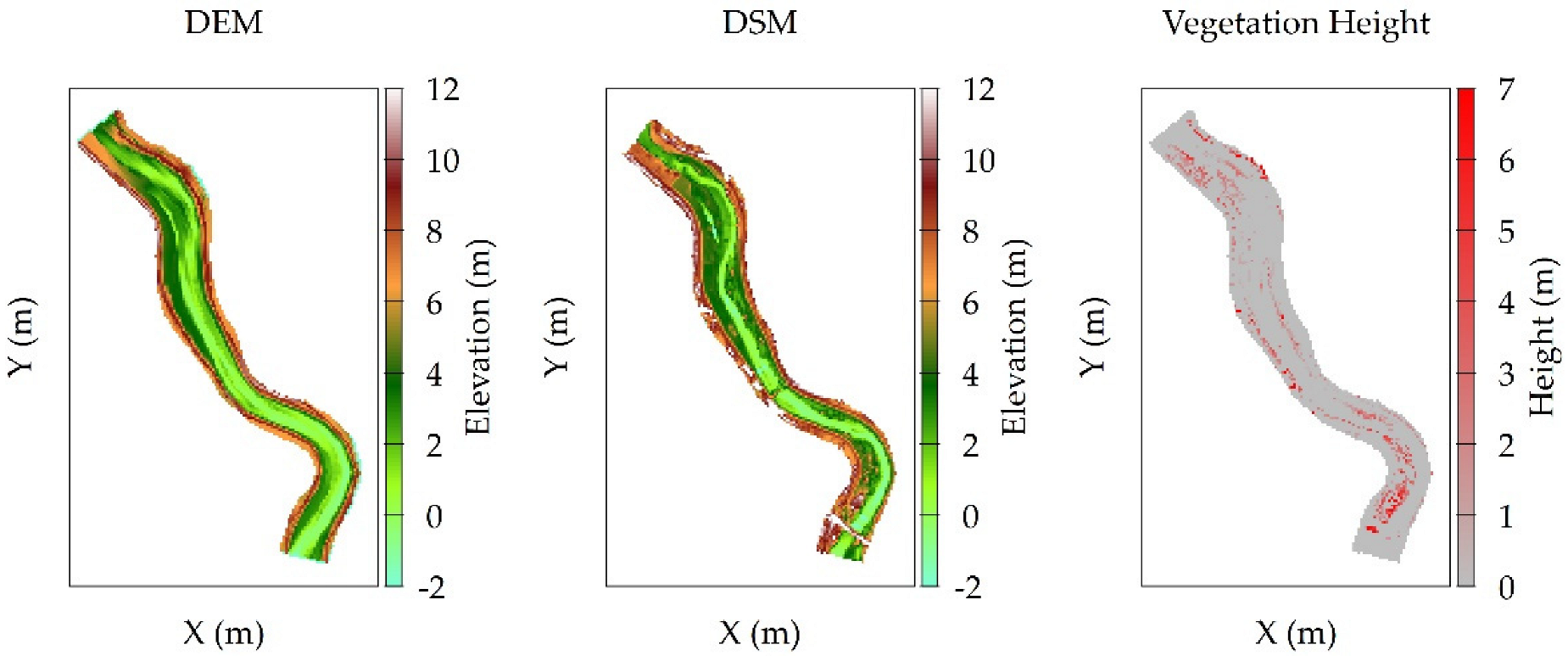
Figure 5 illustrates the DSM, DEM, and vegetation height as per the UAV observations from September 2019. From this image, the clear difference between the DSM and the DEM in the vegetated pixels is shown, expressing the vegetation height.

Figure 5.
Image of the DEM (left), DSM (center), and vegetation height (right); vegetation height is the result of DSM–DEM for the vegetated grid cells.
The vegetation area and height varied significantly with the passing of seasons. The vegetation area has been shown to follow a clear pattern of variation according to the seasons. The highest area coverage was observed in the summer, when precipitation and temperature are high. In contrast, with low temperature and precipitation, the winter showed the lowest amount of vegetation coverage area. The average height also showed a similar pattern of variation, although less accentuated than the area. Figure 6 shows the values of area and average height for each month from April 2020 to March 2021.
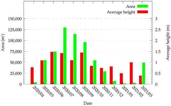
Figure 6.
Vegetated area and vegetation average height in the UAV-observed stretch shown in Figure 1c from April 2020 to March 2021.
4.2. Hydrologic Simulation
The results of the RRI model simulation conformed to the observed data. The simulated hydrograph in the outlet revealed a peak discharge of approximately 1250 m3 s–1, lower than the 100-year return period of 1650 m3 s–1 affirmed by Tanaka et al. [26]. Figure 7 shows the discharge in each station, in the upstream section of the UAV-observed area and the outlet. The comparison between the observed and simulated water level in each station is shown in Figure 8. Nash–Sutcliffe efficiency and RMSE were calculated for each station to validate the model. Except for the Kawazaki station, all stations showed Nash–Sutcliffe values ranging from 0.62 to 0.88. Because the Nash–Sutcliffe efficiency of most of the gauge stations was close to 1, the model could be considered sufficiently accurate.
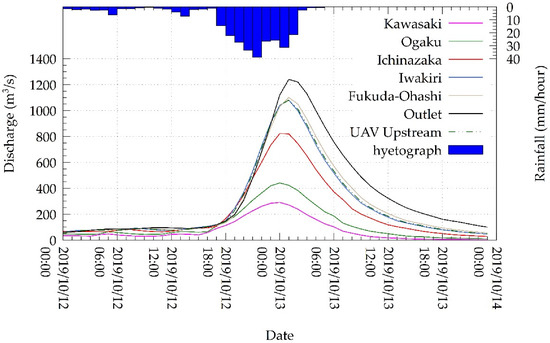
Figure 7.
RRI simulated discharges in all the water level gauge stations shown in Figure 1b, in the UAV upstream section, and in the outlet.
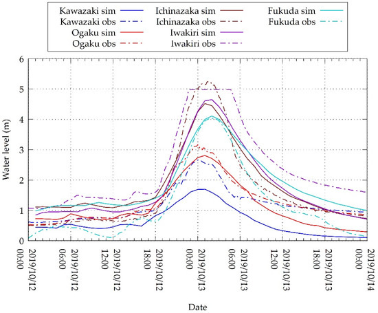
Figure 8.
Comparisons between the RRI simulated and observed water levels in the 5 gauge stations.
The results of the simulation were like those of Bhagabati and Kawasaki [32], producing a reasonable discharge while overestimating the flooded area on a flat region of the river basin. The peak inundation (Figure 9) showed a virtual inundation in the residential area west of the Nanakita River between the Iwakiri and Fukuda Ohashi stations. This overestimation occurred because the model did not consider the city’s drainage system. In the same stretch, a small flood was also observed because the model did not consider the flood control structures. Thus, a minor reduction in the discharge occurred from the Iwakiri to the following station, Fukuda Ohashi. This result contradicts those of Nastiti et al. [31], which produced a realistic inundated area but unrealistic discharge.
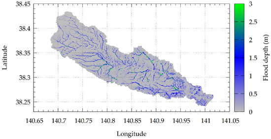
Figure 9.
RRI-simulated peak inundation caused by the typhoon event in the river basin shown in Figure 1b.
4.3. Hydraulic Simulation
Considering the vegetation conditions of September 2019, the dynamic roughness model simulated a higher water level profile than that of the static roughness model. Both results were compared with the observed peak water level at specific locations. The dynamic roughness model obtained a more precise result, obtaining an RMSE of 0.17 m compared with that of 0.67 m produced by the static roughness simulations. As proposed by Ebrahimi et al. [2], the adoption of a non-constant Manning roughness coefficient routine improved the quality of the results, which are also in agreement with the results obtained by Mohammadi and Kashefipour [13]. The increased higher accuracy obtained from the dynamic roughness model demonstrates that, as in Yoshida et al. [14], the distributed vegetation in the reach can be considered a good parameter to calculate the roughness in the reach scale.
As shown in Figure 10, the water level in the dynamic roughness simulation increased by 7.03% on average compared with that in the static roughness simulation. The absolute water levels increased by 57 cm at 500 m and 39 cm at 2000 m from the downstream end. The water level increased by a maximum height of 61 cm at 700 m from the downstream boundary. These differences in the actual flood levels evidenced using the dynamic roughness calculation routine confirmed the statement of Wu et al. [8] regarding the consequences of using a constant roughness coefficient, demonstrating that the set Manning roughness coefficient value of 0.038 for the floodplain areas in the static roughness simulation was not enough to represent the vegetation effect in this river stretch.
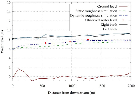
Figure 10.
Simulated water level profiles of the simple Manning roughness coefficient setting simulation and the dynamic Manning roughness coefficient calculation simulation.
Measuring the increase in the water level is important for the prediction of areas with greater likelihood of overtopping, aiding in flood vulnerability assessment. The results of the dynamic roughness adaptation in the 2D model prove its usefulness in urban flood control and inundation prediction. The proposed model is better suited for preparedness once it has predicted a worsened and more realistic scenario.
Sensitivity analysis of the Manning value in the floodplain areas was performed in the static roughness model aiming to achieve a roughness value that better represents the roughness caused by the vegetation and other surfaces. The comparison between observed and simulated water levels in each case is presented in Figure 11. As expected, increasing the Manning value in the floodplains brought the water level profile closer to the observed values, and validated the previous statement that Manning of 0.038 was not enough to represent the roughness in the location. RMSE was calculated for each simulation and the values are demonstrated in Table 2.
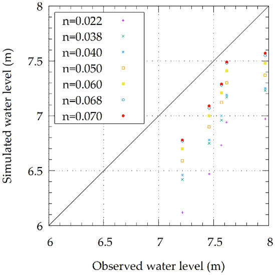
Figure 11.
Comparison of simulated and observed water level values from the static roughness model using several Manning values.

Table 2.
RMSE values achieved by the different floodplain Manning values of each simulation.
As shown in Table 2 and Figure 11, the Manning of 0.070 was the value that most approached the observed water level, better representing the effect of the floodplain roughness, with the RMSE of 0.340, although, this error is still larger than RMSE obtained from the dynamic roughness model.
The behavior of the Manning roughness coefficient in the vegetated grid cells in the dynamic roughness model can be seen in Figure 12a,b, where the comparison between the variation in the Manning roughness coefficient of two different grid cells is shown. In Figure 12c,d, the Manning values of the static model in same cells is demonstrated. The results confirmed what could be observed in Wu et al. [8], that the Manning roughness coefficient value is inversely proportional to the water depth. Figure 12a shows a channel grid cell. In that case, because the water rapidly submerges the vegetation, the calculation routine is activated from the start of the simulation. It shows that while the water depth increases, the Manning roughness coefficient value decreases until the peak water depth. In contrast, when the water level starts to decrease, the Manning roughness coefficient value starts to increase. Figure 12b at the right shows the Manning roughness coefficient behavior in a floodplain grid cell. It can be noticed that until the 22nd hour of the simulation, the water did not fully submerge the vegetation, and therefore the water was trapped in the cell and the value was not calculated. Once the degree of submergence was higher than 1, the values were calculated, ranging from 0.05 to 0.1, confirming once more that the value of 0.038 considered in the static roughness simulation was not high enough to represent the vegetation. While the variation of Manning values can be observed in Figure 12a,b, the values are constant in Figure 12c,d, which represent the static roughness model.
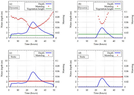
Figure 12.
Pixel-level behavior of the Manning roughness coefficient estimation along the simulation time for: (a) the dynamic roughness model in September 2019 at point 1 from Figure 1c, (b) the dynamic roughness model in September 2019 at point 2 from Figure 1c, (c) the static roughness model at point 1 in Figure 1c, and (d) the static roughness model at point 2 in Figure 1c.
The use of the dynamic roughness calculation routine based on the degree of submergence of the vegetation provoked considerable fluctuations in the Manning roughness coefficient. The rapid and intense increase in the discharge caused a fast rise of the water level, drastically altering the Manning roughness coefficient in the grid cells. During the beginning of the event, before the water level reached its peak, the degree of submergence of the vegetation increased, reducing the Manning roughness coefficient, to the point where it reached its lowest values. Toward the end of the typhoon event, the discharge decreased, reducing the water level and the degree of submergence of the plants, causing an increase in the Manning roughness coefficient.
The main advantage of the dynamic roughness model is that it does not require the same calibration process as the static roughness model since the Manning values are calculated from the vegetation itself. In addition, by using dynamic Manning in the vegetated grid cells, the effect of the vegetation can be assessed in the model, in contrast to the static roughness model. As discussed in Ebrahimi et al. [2], the use of a constant Manning cannot fully express the effect of the vegetation on the flow dynamics. Nevertheless, there are factors that limit the application of the dynamic roughness model. Firstly, Equation (5) unified different types of shrubs and tall grass vegetation under a single curve, not considering the effect of trees and neglecting that different patches of vegetation types would have local effects on the roughness. The vegetation height in each grid cell is constant, not considering the plant flexibility, which also provokes variations on the Manning value, as seen in [12]. Furthermore, the blockage of water in vegetated grid cells restrain the model applicability in scenarios where the vegetation is emergent for long periods. Therefore, the applicability of the dynamic roughness model is restrained to scenarios where the flow depth is predominantly higher than the vegetation and in which there are large fluctuations of water level and a considerable amount of vegetation. The model is especially useful when the degree of submergence remains low for long periods, when the roughness value is larger and has more influence on the flow dynamics. For flood scenarios in which the discharge remains very high for longer periods, the high degree of submergence tends to provide a lower Manning roughness coefficient, causing little influence in the flow dynamics. In addition, regarding the types of vegetation, the model should be considered only in river stretches where the vegetation is mostly comprised of shrubs and tall grass.
4.4. Seasonal Effect of Vegetation on the Water Profile
In Song et al. [15], the estimation of the year-round seasonal Manning roughness coefficient variation was performed by calibrating the Manning roughness coefficient value through trial and error for a month as a single value along the entire river stretch to match the flow condition for that month. The proposed model determined the Manning roughness coefficient from the vegetation characteristics of the floodplains rather than by trial and error, simulating the effect of the vegetation on the water level from April 2020 to March 2021.
The results of the simulations demonstrated that water level significantly varies due to changes in the vegetation area and height. The variation of roughness observed by the water level change occurred in conformity to the Manning roughness coefficient variation observed in Song et al. [15], showing the peak water level in the summer period and the lowest in the winter. Figure 13a,b depict the peak water level simulated for each month in the central section of the stretch compared with the variation in the vegetation height and area, respectively.
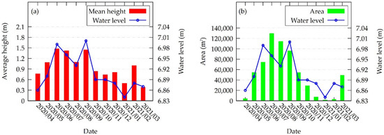
Figure 13.
Water level profiles simulated by the 2D hydraulic model using the dynamic roughness model with: (a) the vegetation average height and (b) vegetation area from April 2020 to March 2021.
The seasonal variation of the vegetated area generally agrees with the water level variation and this agreement is also observed regarding the variation of the average height of the vegetation. In agreement with de Doncker et al. [43], the results demonstrate that the increase in vegetation further roughens the channel, triggering an increase in the water level. Furthermore, the large seasonal variation in the vegetation area and height substantially alters the roughness.
A linear relationship between the water level and the vegetation area and height can be seen in Figure 14a,b, respectively. The correlation coefficient (R) and the coefficient of determination (R2) of vegetation average height versus water level were 0.91 and 0.83, respectively, confirming a stronger relationship than that of the vegetation area versus water level, with R of 0.79 and R2 of 0.63. The parameters are dependent on each other, influencing the overall Manning roughness coefficient of the floodplains.
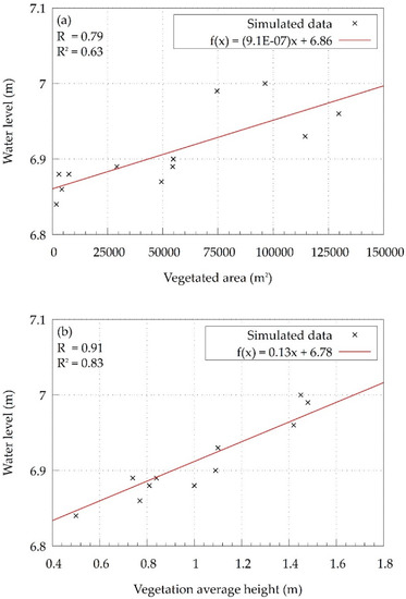
Figure 14.
Linear relationship between the water level in the middle section of the UAV observed area and the vegetation parameters: (a) area; (b) average height.
5. Conclusions
The riparian vegetation in the UAV-observed 2 km stretch of the Nanakita River greatly varies in coverage area and height throughout the passing of the seasons. Identifying the vegetation using the MLP algorithm has achieved an accuracy of 99% for summer and spring and 96% for autumn and winter, which represents a useful aid for riparian vegetation classification. As in Casado et al. [17], the results show that artificial intelligence algorithms are powerful tools for river mapping and management. The lower recall of 74% obtained for autumn and winter demonstrates that classifying vegetation during the period of foliage loss is a challenging task. This happens because of the confusion of the vegetation color with that of other features present in the orthoimages.
The dynamic and static roughness models obtained RMSEs of 0.17 m and 0.67 m, respectively, leading to the conclusion that the dynamic roughness model achieved a more realistic simulation of Typhoon Hagibis than the static roughness model did. This demonstrates that the consideration of a fluctuating Manning roughness coefficient based on the degree of submergence of the plants improved the simulation results, as suggested by previous studies [2,5,8]. As predicted by Wu et al. [8], the use of varied Manning roughness coefficient values provoked considerable discrepancies in the simulated water levels. The largest difference of the simulated water level between the static model and the dynamic model was 61 cm, with the higher water level being predicted by the dynamic roughness model. The dynamic roughness model was shown to improve the safety for flood vulnerability studies in the Nanakita River.
Seasonal variations in vegetation area and height have a clear effect on the flow dynamics of the river. From the results of the simulations, it could be concluded that the water level is proportional to the amount of vegetation in the riparian zones. The highest water level was obtained in the summer, when the vegetation volume is at its peak, and the lowest value during the winter, when there is less vegetation. A low water level was also simulated in the early spring season, in April 2020, owing to the removal of the plants by Miyagi prefecture in October 2019, after the typhoon event.
The vegetation area and average height were demonstrated to have a good correlation with the simulated water levels, with average height achieving the strongest relationship, with an R of 0.91 and R2 of 0.83. Therefore, considering only the vegetation area to estimate the water level, as does the static roughness model, would be less efficient. Considering the distributed vegetation height together with the vegetation area provides a stronger relationship between the riparian vegetation and the water level.
The method to obtain the vegetation location and its distributed height, with the consideration of the parameters in the dynamic roughness model proposed in this study was proven to be applicable for the purpose of river management in Nanakita River.
In the future, the limitations of the dynamic roughness model will be addressed. The identification of the different types of vegetation in the floodplains will be performed; thus, vegetation flexibility and the flow in emergent conditions will be considered in the model. Therefore, the applicability of the model will be broader, and it can be tested in other locations.
Author Contributions
Conceptualization, A.A.F. and M.H.; methodology, A.A.F., M.H. and K.U.; software, A.A.F. and M.H.; validation, A.A.F., M.H., K.U., K.I. and S.S.; investigation, A.A.F., M.H., K.U. and K.I.; resources, M.H., K.U. and K.I.; writing—original draft preparation, A.A.F.; writing—review and editing, A.A.F., M.H. and K.U.; supervision, M.H. and K.U.; project administration, K.U. and S.S.; funding acquisition, K.U. All authors have read and agreed to the published version of the manuscript.
Funding
This research was supported by a collaboration research fund of International Research Institute of Disaster Science, Tohoku University and Fukken Gijyutsu Consultants Co., Ltd.
Institutional Review Board Statement
Not applicable.
Informed Consent Statement
Not applicable.
Data Availability Statement
Not applicable.
Acknowledgments
The authors acknowledge the support of the Miyagi prefecture for providing the water depth data of the Nanakita River used for the model validation, as well as the cross-sections of the river used to generate the terrain topography.
Conflicts of Interest
The authors declare no conflict of interest.
References
- Cowan, W.L. Estimating hydraulic roughness coefficients. Agric. Eng. 1956, 37, 473–475. [Google Scholar]
- Ebrahimi, N.G.; Fathi-Moghadam, M.; Kashefipour, S.M.; Saneie, M.; Ebrahimi, K. Effects of flow and vegetation states on river roughness coefficients. J. Appl. Sci. 2008, 8, 2118–2123. [Google Scholar] [CrossRef][Green Version]
- Darby, S.E. Effect of riparian vegetation on flow resistance and flood potential. J. Hydraul. Eng. 1999, 125, 443–454. [Google Scholar] [CrossRef]
- Sun, X.; Shiono, K.; Rameshwaran, P.; Chandler, J.H. Modelling vegetation effects in irregular meandering river. J. Hydraul. Res. 2010, 48, 775–783. [Google Scholar] [CrossRef]
- Nikora, V.; Larned, S.; Nikora, N.; Debnath, K.; Cooper, G.; Reid, M. Hydraulic resistance due to aquatic vegetation in small streams: Field study. J. Hydraul. Eng. 2008, 134, 1326–1332. [Google Scholar] [CrossRef]
- Wang, P.; Wang, C.; Zhu, D.Z. Hydraulic resistance of submerged vegetation related to effective height. J. Hydrodynam. 2010, 22, 265–273. [Google Scholar] [CrossRef]
- Wilson, C.A.M.E. Flow resistance models for flexible submerged vegetation. J. Hydrol. 2007, 342, 213–222. [Google Scholar] [CrossRef]
- Wu, F.-C.; Shen, H.W.; Chou, Y.-J. Variation of roughness coefficients for unsubmerged and submerged vegetation. J. Hydraul. Eng. 1999, 125, 934–942. [Google Scholar] [CrossRef]
- Devi, T.B.; Kumar, B. Experimentation on submerged flow over flexible vegetation patches with downward seepage. Ecol. Eng. 2016, 91, 158–168. [Google Scholar] [CrossRef]
- Jalonen, J.; Järvelä, J.; Aberle, J. Leaf area index as vegetation density measure for hydraulic analyses. J. Hydraul. Eng. 2013, 139, 461–469. [Google Scholar] [CrossRef]
- Schoneboom, T.; Aberle, J.; Dittrich, A. Hydraulic resistance of vegetated flows: Contribution of bed shear stress and vegetative drag to total hydraulic resistance. In River Flow; Dittrich, A., Koll, K., Aberle, J., Geisenhainer, P., Eds.; Bundesanstalt für Wasserbau: Karlsruhe, German, 2010; pp. 269–276. ISBN 978-3-939230-00-7. [Google Scholar]
- Caroppi, G.; Järvelä, J. Shear layer over floodplain vegetation with a view on bending and streamlining effects. Environ. Fluid Mech. 2022, 22, 587–618. [Google Scholar] [CrossRef]
- Mohammadi, S.; Kashefipour, S.M. Numerical modeling of flow in riverine basins using an improved dynamic roughness coefficient. Water Resour. 2014, 41, 412–420. [Google Scholar] [CrossRef]
- Yoshida, K.; Maeno, S.; Ogawa, S.; Mano, K.; Nigo, S. Estimation of distributed flow resistance in vegetated rivers using airborne topo-bathymetric LiDAR and its application to risk management tasks for Asahi River flooding. J. Flood Risk Manag. 2020, 13, e12584. [Google Scholar] [CrossRef]
- Song, S.; Schmalz, B.; Xu, Y.P.; Fohrer, N. Seasonality of roughness—The indicator of annual river flow resistance condition in a lowland catchment. Water Resour. Manag. 2017, 31, 3299–3312. [Google Scholar] [CrossRef]
- Carbonell-Rivera, J.P.; Estornell, J.; Ruiz, L.A.; Torralba, J.; Crespo-Peremarch, P. Classification of UAV-based photogrammetric point clouds of riverine species using machine learning algorithms: A case study in the Palancia River, Spain. Int. Arch. Photogramm. Remote Sens. Spatial Inf. Sci. 2020, XLIII-B2-2020, 659–666. [Google Scholar] [CrossRef]
- Casado, M.R.; Gonzalez, R.B.; Kriechbaumer, T.; Veal, A. Automated identification of river hydromorphological features using UAV high resolution aerial imagery. Sensors 2015, 15, 27969–27989. [Google Scholar] [CrossRef]
- Javernick, L.; Brasington, J.; Caruso, B. Modeling the topography of shallow braided rivers using structure-from-motion photogrammetry. Geomorphology 2014, 213, 166–182. [Google Scholar] [CrossRef]
- van Iersel, W.; Straatsma, M.; Addink, E.; Middelkoop, H. Monitoring height and greenness of non-woody floodplain vegetation with UAV time series. ISPRS J. Photogramm. Remote Sens. 2018, 141, 112–123. [Google Scholar] [CrossRef]
- Forlani, G.; Dall’Asta, E.; Diotri, F.; di Cella, U.M.; Roncella, R.; Santise, M. Quality assessment of DSMs produced from UAV flights georeferenced with on-board RTK positioning. Remote Sens. 2018, 10, 311. [Google Scholar] [CrossRef]
- Zahidi, I.; Yusuf, B.; Cope, M. Vegetative roughness estimation for hydraulic modelling: A review. Res. Civ. Environ. Eng. 2014, 2, 1–10. [Google Scholar]
- Shakti, P.C.; Hirano, K.; Iizuka, S. Flood inundation mapping of the Hitachi region in the Kuji River basin, Japan, during the October 11–13, 2019 extreme rain event. J. Disaster Res. 2020, 15, 712–725. [Google Scholar] [CrossRef]
- MLITT. National Land Data Information. Ministry of Land, Infrastructure, Transport and Tourism. Available online: https://nlftp.mlit.go.jp/ksj/gml/datalist/KsjTmplt-L03-b_r.html (accessed on 7 August 2022).
- Moriguchi, S.; Matsugi, H.; Ochiai, T.; Yoshikawa, S.; Inagaki, H.; Ueno, S.; Suzuki, M.; Tobita, Y.; Chida, T.; Takahashi, K.; et al. Survey report on damage caused by 2019 Typhoon Hagibis in Marumori Town, Miyagi Prefecture, Japan. Soils Found. 2021, 61, 586–599. [Google Scholar] [CrossRef]
- Tali, M.G.; Tavakolinia, J.; Heravi, A.M. Flood vulnerability assessment in northwestern areas of Tehran. J. Disaster Res. 2016, 11, 699–706. [Google Scholar] [CrossRef]
- Tanaka, H.; Adityawan, M.B.; Mano, A. Morphological changes at the Nanakita River mouth after the Great East Japan Tsunami of 2011. Coast. Eng. 2014, 86, 14–26. [Google Scholar] [CrossRef]
- Viet, N.T.; Tanaka, H.; Nakayama, D.; Yamaji, H. Effect of morphological changes and waves on salinity intrusion in the Nanakita River mouth. Proc. Hydraul. Eng. 2006, 50, 139–144. [Google Scholar] [CrossRef][Green Version]
- Pilailar, S.; Sakamaki, T.; Izumi, N.; Tanaka, H.; Nishimura, O. The characteristic change of fine particulate organic matter due to a flood in the Nanakita River. Proc. Hydraul. Eng. 2003, 47, 1033–1038. [Google Scholar] [CrossRef][Green Version]
- Japan Dam Foundation. Nanakita Dam [Miyagi Pref.]—Dams in Japan. Available online: http://damnet.or.jp/cgi-bin/binranA/enAll.cgi?db4=0302 (accessed on 7 August 2022).
- Sato, S.; Kure, S.; Moriguchi, S.; Udo, K.; Imamura, F. Online information as real-time big data about heavy rain disasters and its limitations: Case study of Miyagi Prefecture, Japan, during Typhoons 17 and 18 in 2015. J. Disaster Res. 2017, 12, 335–346. [Google Scholar] [CrossRef]
- Nastiti, K.D.; Kim, Y.; Jung, K.; An, H. The application of rainfall-runoff-inundation (RRI) model for inundation case in upper Citarum watershed, West Java-Indonesia. Procedia Eng. 2015, 125, 166–172. [Google Scholar] [CrossRef]
- Bhagabati, S.; Kawasaki, A. Consideration of the rainfall-runoff-inundation (RRI) model for flood mapping in a deltaic area of Myanmar. Hydrol. Res. Lett. 2017, 11, 155–160. [Google Scholar] [CrossRef]
- San, Z.M.L.T.; Zin, W.W.; Kawasaki, A.; Acierto, R.A.; Oo, T.Z. Developing flood inundation map using RRI and SOBEK models: A case study of the Bago River basin, Myanmar. J. Disaster Res. 2020, 15, 277–287. [Google Scholar] [CrossRef]
- Sayama, T.; Ozawa, G.; Kawakami, T.; Nabesaka, S.; Fukami, K. Rainfall–runoff–inundation analysis of the 2010 Pakistan flood in the Kabul River basin. Hydrol. Sci. J. 2012, 57, 298–312. [Google Scholar] [CrossRef]
- Ishizaki, H.; Matsuyama, H. Distribution of the annual precipitation ratio of radar/raingauge-analyzed precipitation to AMeDAS across Japan. SOLA 2018, 14, 192–196. [Google Scholar] [CrossRef]
- Yamazaki, D.; Ikeshima, D.; Sosa, J.; Bates, P.D.; Allen, G.H.; Pavelsky, T.M. MERIT hydro: A high-resolution global hydrography map based on latest topography dataset. Water Resour. Res. 2019, 55, 5053–5073. [Google Scholar] [CrossRef]
- Iwasa, Y.; Inoue, K. Mathematical simulations of channel and overland flood flows in view of flood disaster engineering. J. Nat. Disaster Sci. 1982, 4, 1–30. [Google Scholar]
- Inoue, K.; Nakagawa, H.; Toda, K. Numerical analysis of overland flood flows by means of one-and two-dimensional models. In Proceedings of the 5th JSPS-VCC Seminar on Integrated Engineering, Engineering Achievement and Challenges, Johor Bahru, Malaysia, 12–14 November 1994; pp. 388–397. [Google Scholar]
- Hashimoto, M.; Yoneyama, N.; Kawaike, K.; Deguchi, T.; Hossain, M.A.; Nakagawa, H. Flood and substance transportation analysis using satellite elevation data: A case study in Dhaka City, Bangladesh. J. Disaster Res. 2018, 13, 967–977. [Google Scholar] [CrossRef]
- Japan Institute of Country-ology and Engineering. Manual of plans for river channel (in Japanese). In Manual of Plans for River Channel; Sankaidou: Tokyo, Japan, 2002. [Google Scholar]
- Arcement, G.J.; Schneider, V.R. Guide for Selecting Manning’s Roughness Coefficients for Natural Channels and Flood Plains; Water Supply Paper 2339; United States Federal Highway Administration: Washington, DC, USA, 1989; pp. 1–44. [CrossRef]
- Weidner, U.; Förstner, W. Towards automatic building extraction from high-resolution digital elevation models. ISPRS J. Photogramm. Remote Sens. 1995, 50, 38–49. [Google Scholar] [CrossRef]
- de Doncker, L.; Troch, P.; Verhoeven, R.; Bal, K.; Meire, P.; Quintelier, J. Determination of the Manning roughness coefficient influenced by vegetation in the river Aa and Biebrza river. Environ. Fluid Mech. 2009, 9, 549–567. [Google Scholar] [CrossRef]
Publisher’s Note: MDPI stays neutral with regard to jurisdictional claims in published maps and institutional affiliations. |
© 2022 by the authors. Licensee MDPI, Basel, Switzerland. This article is an open access article distributed under the terms and conditions of the Creative Commons Attribution (CC BY) license (https://creativecommons.org/licenses/by/4.0/).


