Article

A GIS-Based Comparative Analysis of Frequency Ratio and Statistical Index Models for Flood Susceptibility Mapping in the Upper Krishna Basin, India

1
Department of Geography, HPT Arts and RYK Science College, Nashik 422005, Maharashtra, India
2
Department of Geography, Faculty of Humanities and Social Sciences, Chiang Mai Rajabhat University, Mueang, Chiang Mai 50300, Thailand
3
Institute for Sustainable Industries & Livable Cities, Victoria University, P.O. Box 14428, Melbourne, VIC 8001, Australia
4
College of Engineering and Science, Victoria University, P.O. Box 14428, Melbourne, VIC 8001, Australia
5
Department of Civil Engineering, Faculty of Engineering, Sri Lanka Institute of Information Technology, Malabe 10115, Sri Lanka
*
Authors to whom correspondence should be addressed.
Water 2022, 14(22), 3771; https://doi.org/10.3390/w14223771
Submission received: 1 November 2022 / Revised: 17 November 2022 / Accepted: 18 November 2022 / Published: 20 November 2022
(This article belongs to the Section Hydrology)

Abstract

:
The Upper Krishna Basin in Maharashtra (India) is highly vulnerable to floods. This study aimed to generate a flood susceptibility map for the basin using Frequency Ratio and Statistical Index models of flood analysis. The flood hazard inventory map was created by 370 flood locations in the Upper Krishna Basin and plotted using ArcGIS 10.1 software. The 259 flood locations (70%) were selected randomly as training samples for analysis of the flood models, and for validation purposes, the remaining 111 flood locations (30%) were used. Flood susceptibility analyses were performed based on 12 flood conditioning factors. These were elevation, slope, aspect, curvature, Topographic Wetness Index, Stream Power Index, rainfall, distance from the river, stream density, soil types, land use, and distance from the road. The Statistical Index model revealed that 38% of the area of the Upper Krishna Basin is in the high- to very-high-flood-susceptibility class. The precision of the flood susceptibility map was confirmed using the receiver operating characteristic and the area under the curve value method. The area under the curve showed a 66.89% success rate and a 68% prediction rate for the Frequency Ratio model. However, the Statistical Index model provided an 82.85% success rate and 83.23% prediction rate. The comparative analysis of the Frequency Ratio and Statistical Index models revealed that the Statistical Index model was the most suitable for flood susceptibility analysis and mapping flood-prone areas in the Upper Krishna Basin. The results obtained from this research can be helpful in flood disaster mitigation and hazard preparedness in the Upper Krishna Basin.

1. Introduction

Floods are well-known catastrophic hydro-meteorological disasters that cause huge damage to human life, settlements and industries, agriculture and animals, and the economy [1,2,3,4,5,6,7]. Globally, about 170 million people have been affected due to floods every year [8,9]. Under climate change, the frequency and magnitude of floods have increased significantly due to environmental degradation, excessive growth of the population, urbanization, and changing land use pattern [10,11]. According to Alfieri et al. [12], the frequency of floods has increased by over 40% in the last two decades throughout the world, which has caused damages of about 75 billion USD per year. Although measuring the magnitude and reporting the destruction because of inundation are enormously challenging [2], assessments and approximations of floods have significantly increased [13,14]. To minimize potential losses to the natural and artificial environment because of floods, flood prevention is essential [15]. Therefore, recognizing and plotting flood susceptibility zones significantly help with flood early warning systems, flood management and mitigation, emergency services, and disaster risk reduction [16,17,18,19]. Many scholars have conducted studies on Flood Susceptibility Mapping (FSM) using Remote Sensing (RS) and Geographical Information Systems (GISs) for flood hazard analysis [20,21,22,23,24,25,26,27].
The FSM includes environmental, geological, geomorphological, meteorological, topographical factors, and soil characteristics [28,29,30,31]. The Logistic Regression (LR), Frequency Ratio (FR), Weight of Evidence (WoE), Statistical Index (SI), Analytical Hierarchy Process (AHP), and Artificial Neural Network (ANN) models have been used by several researchers and government agencies to estimate flood susceptibility precisely [32,33,34,35,36,37,38,39]. Although numerous models have been used for flood susceptibility analysis (FSA), the results obtained by different models varied slightly from region to region. The meteorological and physical characteristics of the river basin are the main factors contributing to floods [40]. Therefore, testing and evaluation of these models can provide optimal and more reliable results [41]. Over the years, statistical methods (LR and SI) have been applied for FSA and natural hazards mapping, and the results of these models are accurate, reliable, and effective for flood disaster management and planning. FR and SI models are simple to run in a GIS environment and can develop valid FSM [27,34,36,37].
India receives more than 75% of its annual rainfall during the monsoon season from June to September [42]. During the monsoon season, flooding in the major rivers of India is the usual phenomenon, for example, the Ganga, Brahmaputra, Narmada, Tapi, Mahi, Godavari, Krishna, and Kaveri Rivers [11,43,44]. According to the NITI Aayog report [45], about 7.17 million hectares of areas of India are affected by floods annually. In addition, about 1.2 million houses are damaged by floods, 1654 human lives are lost, and 618,248 cattle lives are lost annually. The average annual economic losses are Rs 5649 crores. Previous scholars have specified that flood risk zone identification and defensive structural and non-structural risk reduction measures could efficiently decrease flood losses to some extent [46,47]. According to Ullah and Zhang [48], FSM is extensively used to determine flood-prone zones in flood management studies. Therefore, the foremost objective of the present research is a comparative analysis of the FR and SI models for FSM in the Upper Krishna Basin (UKB).

2. Study Area

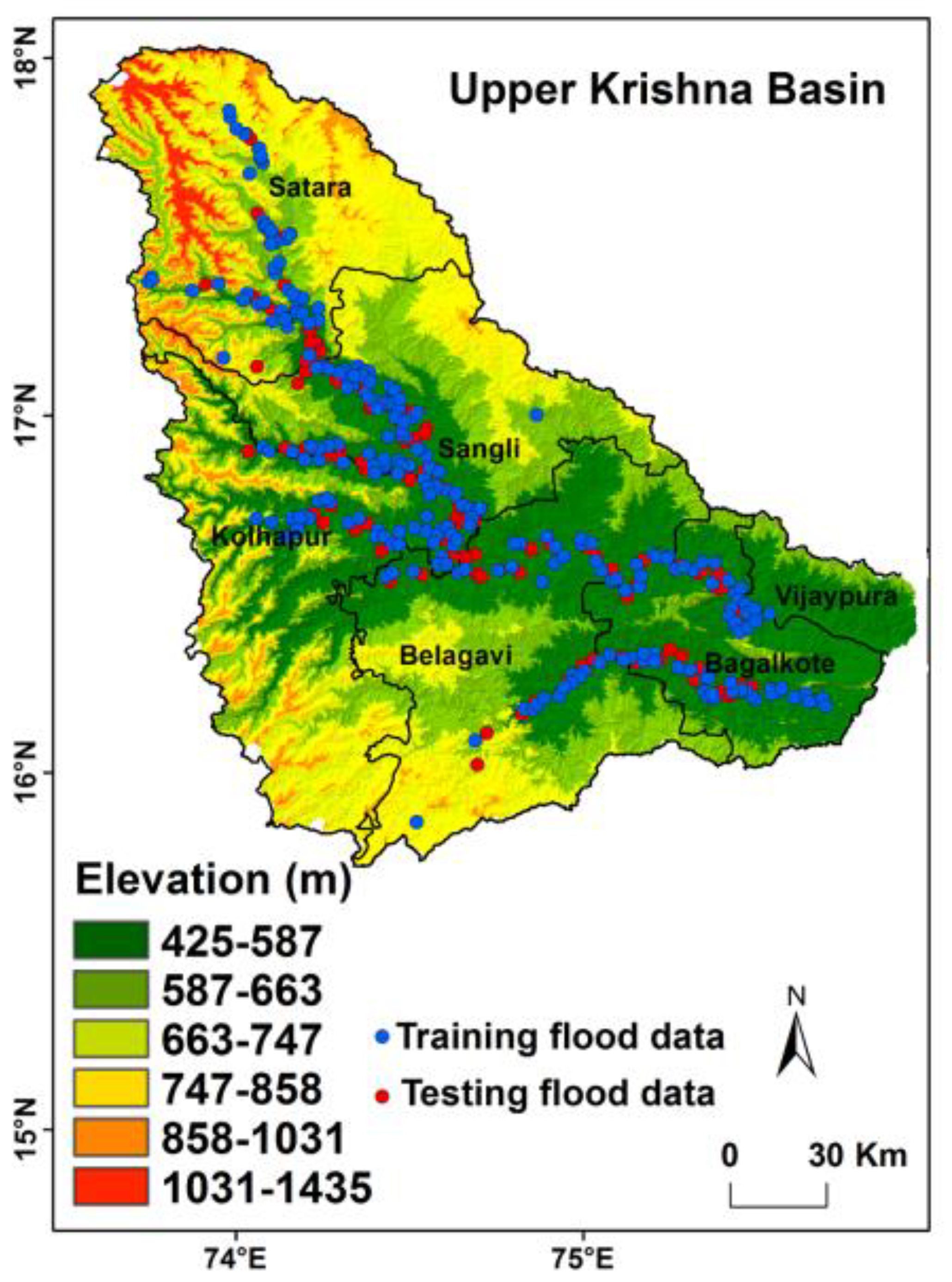
The Krishna Basin is the second-largest river basin in Peninsular India [49] (refer to Figure 1a). The river has its source near Jor village (Mahabaleshwar) at an elevation of 1337 m in Maharashtra. The river flows for a length of 1400 km and joins the Bay of Bengal in Andhra Pradesh. The Krishna Basin extends over the parts of Maharashtra, Karnataka, Telangana, and Andhra Pradesh. The total area of the Krishna Basin is 2.59 Lakh sq. km. The present study is mainly confined to the UKB up to the Almatti Dam in Karnataka [50] (refer to Figure 1b). The UKB covers parts of Satara, Sangli, and Kolhapur districts in Maharashtra and Belagavi, Bagalkote, and Vijaypura districts in Karnataka (refer to Figure 1c). The catchment area above Almatti dam is approximately 35,925 km2 [50]. The major tributaries of Krishna in the upper reaches are Koyna, Warna, Panchganga, Dudhganga, and Ghataprabha. The UKB is roughly triangular. It is entirely covered by Deccan trap lava flows. The alluvium mainly occurs along the banks of Krishna River and its major tributaries and thickness vary from 2 to 20 m. The average annual rainfall (AAR) of the UKB is 1347 mm. Nevertheless, annual rainfall varies from 600 mm to 6208 mm. According to the 2011 census, the total population in the UKB occupying three districts in Maharashtra is about 8,170,973 [51]. In the UKB, the Krishna River and its tributaries are susceptible to recurrent flooding during the monsoon season). Some of the recent devastating floods that occurred in the UKB were in 2005, 2006, 2009, 2011, and 2019. Recently, a disastrous flood hit the UKB in August 2019. The list of the locations affected by the 2019 flood was obtained from various published reports [52,53]. The flood data were classified into training and testing datasets.

3. Materials and Methods

Flood conditioning factors (FCFs) data were obtained from various sources and Table 1 depicts the details. The FSM output was validated by the receiver operating characteristics (ROC) curve. Figure 2 shows a detailed methodology used for FSA.

3.1. Flood Location Data

Flood location data are critical to investigate the association between flood-influencing aspects and flood incidences. The flood inventory map was prepared using the 370 flood locations affected by the August 2019 flood in the UKB (refer to Figure 3). The flood location data were obtained through various reports. The flood sites were classified randomly as training (70%) and (30%) testing sites to build and evaluate the flood models. Accordingly, 259 (111) flood locations were used as training (testing) data.

3.2. Flood Controling Factors

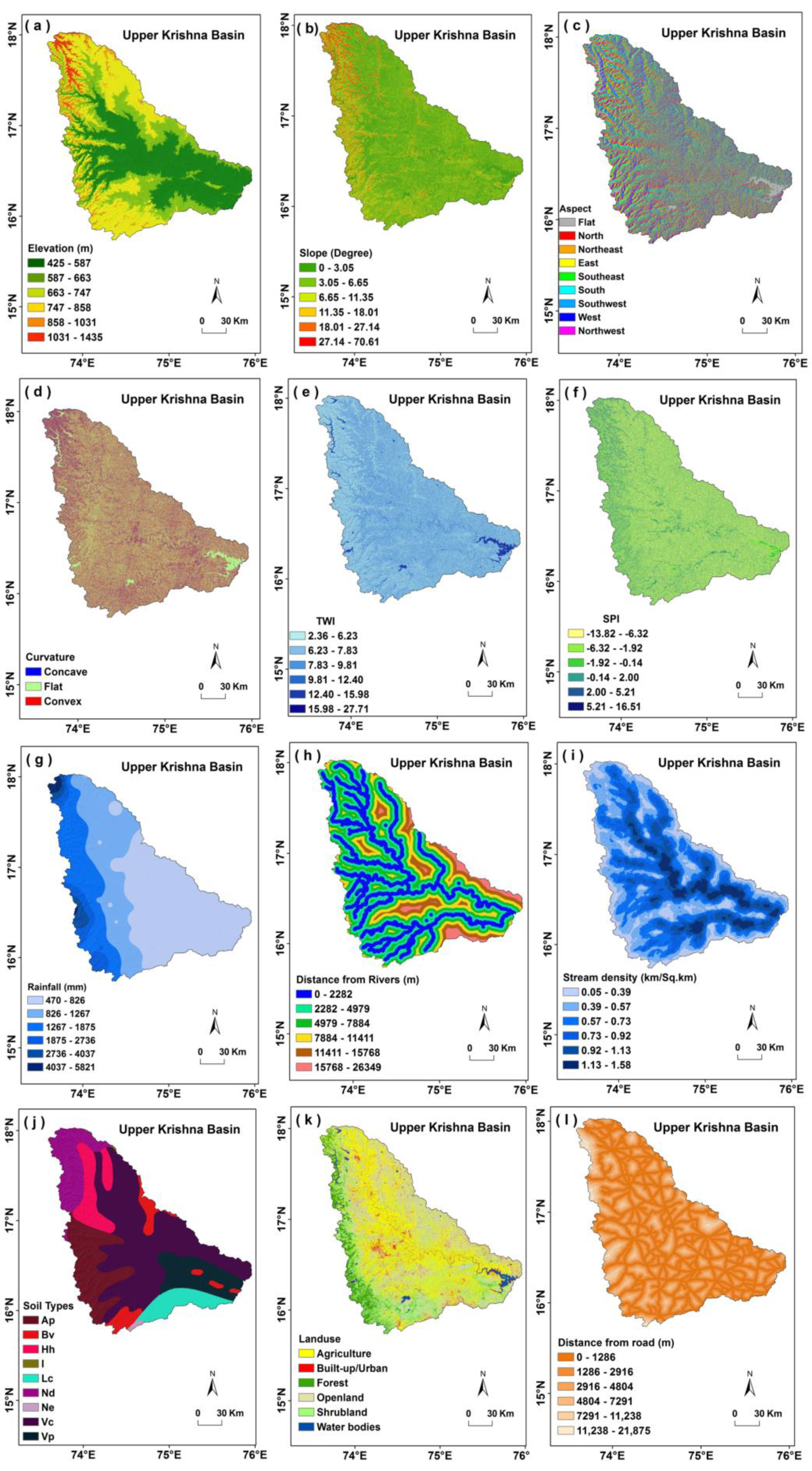
The FCFs were selected based on the area’s physical characteristics, data availability, and literature reviews [54,55,56,57,58]. The analyses of the relationship between flood-controlling elements and flood occurrences required a precise flood inventory map [59]. The flood conditioning parameters comprised elevation, slope, aspect, curvature, Topographic Wetness Index (TWI), Stream Power Index (SPI), rainfall, distance from rivers, stream density, soil types, land use, and distance from the road (refer to Table 1). All factors were converted into raster format with 30 × 30 m spatial resolution. The scaling factors (elevation, slope, TWI, SPI, rainfall, stream density, and distance from the rivers and road) were classified into six classes using the natural breaks classification (refer to Figure 4). The elevation is the most recurrently used key factor for FSM. The lower-elevation areas have a high possibility of flooding and are more susceptible to flood disasters [37,60]. The UKB elevation map was prepared using the Digital Elevation Model (DEM) (refer to Figure 4a). The elevation in the UKB stretched between 425 m and 1435 m. According to Souissi et al. [61], the velocity of surface runoff and the infiltration rate of water are affected by the slope. Therefore, ground slope is essential for FSA and FSM (refer to Table 1). The slope of the basin varied from 0 degrees to 70.61 degrees (refer to Figure 4b). The aspect is one of the crucial FCFs [62]. It influences the received rainfall and shows the direction of the maximum slope of the area surface. The aspect map of the UKB was classified into the 9 classes, and the aspect map of the UKB was created in ArcGIS (refer to Figure 4c). Curvature was categorized into three classes: concave, flat, and convex. According to Young and Mutchler [63], a convex slope can generate considerably extra runoff as compared to a concave slope. Hudson and Kesel [64] (2000) revealed that an area with a curvature value from 1.0 to 2.0 is more susceptible to flooding. The curvature map of the UKB was prepared using ArcGIS 10.1 (refer to Figure 4d). TWI represents the cumulative flow at any point within the watershed. It also denotes the spatial distribution of wetness in the basin. TWI has significance in the FSA and flood mapping [24,36,37,54]. TWI was computed using Equation (1) [23,65] and a TWI map was prepared from the DEM in ArcGIS 10.1 (refer to Figure 4e).
TWI = ln [ A s t a n   B ]
where A s is the cumulative area to a specific pixel and B is the slope angle in degrees. According to Jebur et al. [66], SPI refers to the rate of the erosive power of surface runoff in a specified site in a river basin and can be given in Equation (2). SPI was reclassified into 6 classes and the SPI map for the UKB was generated in ArcGIS 10.1 software (refer to Figure 4f).
SPI   = A s × t a n B
Rainfall is one of the FCFs that is widely used in flood prediction studies [35,36]. The intensity of rainfall in a short period over an area can cause devastating floods [67]. The long-term rainfall data for the UKB were collected from various sources (refer to Table 1). Several scholars have used the Inverse Distance Weighting (IDW) method for spatial and temporal analysis of rainfall [68,69]. Accordingly, the rainfall distribution map of the UKB based on annual average rainfall (AAR) was prepared (refer to Figure 4g). Distance from the rivers controls the magnitude and spread of floods. There is an inverse relation between the distance from the streams and flood spread [61]. In order to measure distance from the rivers, the Euclidean Distance tool in ArcGIS software was used, and the stream density map of the UKB was generated using the DEM (refer to Figure 4h). According to Shekhar and Pandey [70], the risk of flooding increases when drainage density is high. Accordingly, a stream density map of the UKB was prepared using ArcGIS (refer to Figure 4i). Soil types, texture, and organic matter content affect the rates of surface runoff infiltration in the ground [71,72]. Therefore, the soils in the basin play a significant role in flood magnitude and extent. In addition, the water-holding capacity of soils (soil moisture) depends on the characteristics of soils. Soil type and characteristics were studied from the digital global soil data in shapefile format prepared by the Food and Agriculture Organization (FAO) of the United Nations (refer to Figure 4j). Hölting and Coldewey [73] pointed out that floods are also determined by land cover types. The LC affects surface runoff, infiltration rates, time of concentration of rainwater in the basin, and potential flood extent [74,75]. Nevertheless, areas with dense vegetation cover the decrease in the rate of runoff and increase in the percolation rate, whereas a built-up (urban) area obstructs water intrusion into the ground and accelerates the runoff [76,77]. Therefore, LU data of the UKB were obtained from the Landsat-8 images of the 2021 using random forest classification in the Google Earth Engine platform. The LU data were classified into six classes of land use: agriculture, built-up area, forest land, open land, shrub land, and water bodies (refer to Figure 4k). Lastly, distance from the road was derived with the Euclidean Distance tool in ArcGIS and classified into six categories to determine the distance of specific pixels to the nearest road line (refer to Figure 4l).

3.3. Frequency Ratio (FR) Model

The FR is one of the widely used models in various natural hazard (flood, landslide, and forest fire) analyses and mapping [78,79,80,81]. It was used to identify the probabilistic relationship between flood occurrence and FCF. The FR of each conditioning factor class can be expressed as the ratio of the class percentage and the total flood percentage. A greater bivariate probability indicates a stronger correlation, whereas a low FR value means a weak correlation. The FR value is expressed in Equation (3) as follows [34].
F R =   N i j P i j / N P
where FR is the frequency ratio of the sub-classes, N i j is the number of flood locations, P i j is the total number of flood locations in the study area, N is the total number of pixels for each class of the factor, and P is the total number of pixels in the study area. Then, to calculate the flood susceptibility index (FSI), the FR values of each class were combined following Equation (4).
F S I F R = FR
where F S I F R is the flood susceptibility index of the FR method and FR is the total FR values of all classes from each conditioning factor.

3.4. Statistical Index (SI) Model

The statistical index (SI) model was developed by van Westen [82] for landslide susceptibility mapping. SI weight values are calculated using the natural logarithm of the flood existence in each class of the conditioning factor divided by the total flood density in the study area. The higher positive SI value means a strong relationship between flood occurrence and the class of conditioning factors. The negative value shows the low possibility of flooding the class [83]. In this study, the SI weight values of each class of each conditioning factor were obtained using the following Equation (5) [82].
W i j = ln ( D i j D )   = l n [   ( N i j S i j / N S ) ]
where W i j is the statistical index value given to the i class of j factors; D i j is the density of floods over the i class of j factor; D is the total density of floods over the entire area; N i j   is the number of floods in i class of j factor and is the total number of floods in the study area; S i j is the number of pixels in i class of j factor. N is the total number of flood pixels of the study area and S is the total number of pixels of the study area.
The W i j weights were given to conditioning factors using a reclassification method. Finally, the reclassified factors were summed up to generate the flood susceptibility index (FSI) using a raster calculator in the ArcGIS 10.1 software. The FSI calculation is shown by the following Equation (6).
F S I S I = W i j
where F S I S I is the flood susceptibility index of the SI method and W i j are the total W i j values of all classes from each conditioning factor.

3.5. Models Validation

Validation is an essential component in natural hazard susceptibility mapping to check the effectiveness and applicability of the model. This study applied the ROC to signify the graphical association of FSI and the cumulative percentage of flood occurrence. Frequently, ROC and area under ROC curves (AUC) are applied to evaluate the binary response model such as a logistics model [84,85]. They were used for both training data (70%) and testing data (30%). The AUC was also used to calculate the success and prediction rates for training and testing data. The computed results were depicted in the percentage of the study area categorized as FSI (x-axis) versus the cumulative percent of flood occurrence (y-axis). The AUC was calculated using the following equation [86].
A U C = i = 0 n ( x i x i 1 ) y i [ ( x i x i 1 ) ( y i y i 1 ) 2 ]
where x i   is the percentage of the area and y i is the area of the flood. AUC values vary between a maximum value of 1 or 100% and 0.5 or 50%. According to Silalahi et al. [87], based on the AUC value, results can be classified as a very good model (0.9), a good model (0.8–0.9), a medium or reasonable model (0.7–0.8), and a poor model (<0.6).

4. Results and Discussion

4.1. Flood Susceptibility Analysis by the Frequency Ratio Model

The result of the FR was obtained for each sub-class of all flood-controlling factors and is summarized in Table 2. Table 2 shows that the maximum (2.31) FR value with a high flood area (86.87%) for lower elevation class (425–587 m) proves the high probability of flooding in the lower-elevation area of the UKB. Conversely, zero values of FR were observed for the higher elevation classes (858–1031 m and 1031–1435 m) in the basin that signified that these areas have less probability of flooding. Normally, as the elevation increases, the FR value decreases, revealing a high positive relation between FR and flooding events [35]. The slope of the UKB basin has a relationship with flooding events. The steeper slopes produce runoff more quickly toward the downslope. FR values above 1.00 were observed for slopes between 3.05° and 6.65° (1.38) and slopes from 6.65° to 11.35° (1.23), which has the highest susceptibility to flooding. The maximum flood area (52.12%) was observed for a slope varying between 3.05° and 6.65° in the UKB (refer to Table 2). An FR value greater than one is significant for support of flooding [5]. Zero FR values were noted for the higher slopes above 18.01°, which have the lowest susceptibility to flooding in the UKB (refer to Table 2). According to Jaiswal et al. [88], a high slope ultimately increases the flood probability of the flood by increasing the swiftness of discharge, and a high-slope area has less time to infiltrate water in the ground. The slope curvature parameter of floods has a significant effect on flood susceptibility. The maximum FR values of the aspect parameter of flood control were noted for aspects facing southwest (1.67), west (1.37), and northwest (1.17). Therefore, these slope directions had the greatest control on flood occurrence in the basin (refer to Table 2). The concave slopes had the highest FR value (1.17) followed by flat areas with a value of 0.98. About 89% of flood areas were concave and flat in the UKB (refer to Table 2). Khosravi et al. [35] observed maximum flood areas for concave and flat slope areas in the Haraz watershed. In the case of TWI, the first two classes (2.36–6.23 and 6.23–7.83) had an FR of more than 1, which revealed a higher probability of flood occurrences in these zones in the UKB (refer to Table 2). Sharif et al. [89] stated that TWI signifies the influence of landscape on the location and extent of saturated source zones in producing surface runoff in a basin. The maximum FR value (1.46) was observed for the first class of SPI, which varied between −13.82 and −6.32. However, for the remaining classes, the FR was less than one. According to Khosravi et al. [35] the smaller the SPI, the greater the probability of flooding in the basin.
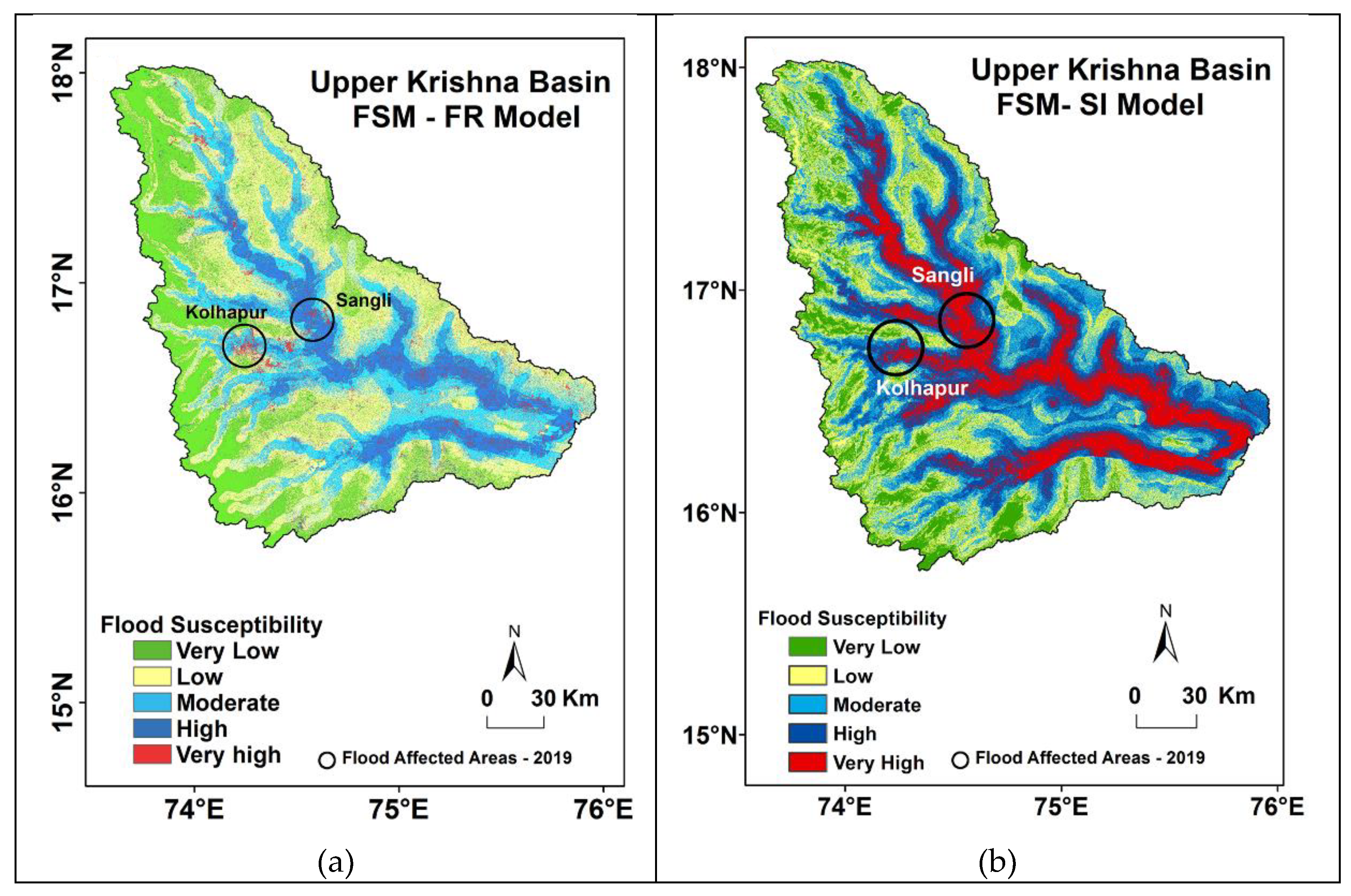
Maximum FR values (above 1) were observed for low-AAR classes (from 470 to 1267 mm) and the FR was zero for the areas with AAR varying between 1875 mm and 5821 mm in the basin (refer to Table 2). This shows that areas with low AAR are more susceptible to flooding as compared to high-AAR areas in the UKB. The distance from the river flood condition factor denoted that the first class of this parameter had the highest FR value (3.03), which suggests that areas from a stream to 2282 m distance are more susceptible to flooding in the UKB (refer to Table 2). In the case of stream density, the high FR values (greater than 1) were noted for areas with stream density varying between 0.73 km/sq.km and 1.58 km/sq.km. This specified that areas with high stream density are more susceptible to flooding than those with less stream density (refer to Table 2). In the UKB, the maximum FR value (2.78) was identified for Pellic Vertisols (Vp) followed by Chromic Vertisols (Vc), which was 1.19 (refer to Table 2). Vertisols soils have a high moisture-holding capacity due to the maximum clay content, which varies between 40 and 80% [90,91]. Therefore, the areas of the UKB with Vertisols soils (Vc and Vp) are more vulnerable to flooding than other types of soils. Land use is a very crucial aspect of the FSA of the UKB. A high FR value (13.36) was noted for the built-up area with about 53% of the flood area (refer to Table 2). The built-up area increases the surface runoff rate and decreases the infiltration rate. This suggests that growth in the urban or built-up area increases flood susceptibility in the UKB basin. The highest FR values for distance from the road were identified for distance classes of 0–1286 m (FR = 1.13) and 1286–2986 m (FR = 1.16), which denoted high flood susceptibility (refer to Table 2). The FSM of the UKB (refer to Figure 5a) was created by categorizing the FSI obtained from the FSA using the FR model. The FSI was classified into five susceptible zones, namely very low susceptibility, low susceptibility, moderate susceptibility, high susceptibility, and very high susceptibility. A proportion of 3% of the area of the UKB fell in the very-high-susceptibility class, while 12% of the area of the basin fell under the high-susceptibility class. Proportions of 25%, 35%, and 25% of the areas of the basin were identified in the moderate, low, and very low classes of susceptibility, respectively (refer to Figure 5a). Overall, areas with low elevation, low slopes, flat curvature, maximum stream density, maximum TWI, low SPI, near the river, highly urbanized, and covered by Vertisols are more susceptible to flooding in the UKB.

4.2. Flood Susceptibility Analysis by the Statistical Index Model

SI model results are summarized in Table 2. Higher positive SI values specify the maximum possibility of flood incidence, and negative values denote a low chance of flood existence in the region. The highest (84) SI value was noted for heights ranging between 425 and 587, whereas with the elevation increase, the SI values either became negative or zero (refer to Table 2). A negative SI value (−28) was observed for a varying slope between 0° and 3.05°. The maximum SI values of the slope class 3.05°–6.65° (SI = 32) and 6.65°–11.35° (SI = 21) revealed that areas between these slopes are more susceptible to flooding (refer to Table 2). A positive SI (16) was obtained for the concave curvature, while negative SI values were identified for the convex (−55) and flat (−2) curvatures. This specified that concave surfaces were more vulnerable to flooding in the UKB (refer to Table 2). The highest value of SI (36) was obtained for the TWI flood factor class between 2.36 and 6.23, and negative and zero SI values were found for TWIs above 7.83 (refer to Table 2). For the SPI, the highest SI (38) was obtained for the class of −13.82 to −6.32, and the negative or zero SI values were noted for the rest of the SPI classes (refer to Table 2). In this study, the highest SI (25) value was observed in the lowest rainfall class (470–826 mm), which was the lowland areas in the east of the UKB. The distance from the river of 0–2282 m displayed the highest SI value (111), while other classes were obtained as negative and zero SI values (refer to Table 2). It is obvious that with the increase in distance from the river, the flood possibility decreases [35]. The area with low stream density gained negative SI values (−299, −311, and −144), while the highest SI value (166) was obtained for the stream density class varying between 1.13 and 1.58 km/sq.km (refer to Table 2). According to the soil type factor, the Vertisols soil showed its influence on flood occurrence with high SI values for Vp (SI = 102) and Vc (SI = 17). With the high content of clay and moisture storage, the area with these soil types is more at risk for flooding. In contrast, negative SI values were observed for the Plinthic Acrisols (Ap), Vertic Cambisols (Bv), Chromic Luvisols (Lc), and Dystric Nitosols (Nd) soils (refer to Table 2). In the case of the land use factor, the highest SI (259) was derived for the built-up area (urban), which occupied 13.36% of the flood area, while negative SI values were observed for agricultural land and open land (refer to Table 2). The maximum SI (15) values observed for the second class (1286 m–2916 m) of the distance from the road showed a highly susceptible area for flooding in the basin. Inclusive, all the flood-controlling factors with high SI increased the probability of flood occurrence in the UKB. Likewise, for the FR model, the FSI was classified into five classes, namely very high, high, moderate, low, and very low (refer to Figure 5b). The FSM generated with the SI model revealed that 16% of the area of the basin was very highly susceptible to floods, whereas 22% of the area of the basin was under a highly susceptible flood zone. The moderate- and low-flood susceptibility classes occupied the same area (25%) of the basin and 13% of the area fell into very low-flood-susceptibility classes (refer to Figure 5b).

4.3. Flood Susceptibility Model Validation and Comparison

Validation of flood susceptibility mapping is essential for flood hazard research. In this research, the FSIs obtained from FR and SI models were validated to compare their performance. ROC-AUC was applied by comparing FSI results with training data (70%) and testing data (30%) to generate success and prediction rates (refer to Figure 6). This method is simple and represents a reliable result, frequently used by many flood hazard studies [34,48]. The success and prediction rate curves are portrayed in Figure 6. The AUC calculation revealed the 66.89% and 82.85% success rates for FR and SI models, respectively. The result of ROC-AUC showed 68% and 83.23% prediction rates for the FR and SI models, respectively. The results validated by the AUC showed an accuracy of the success rate of 82.85% and an accuracy of the prediction rate curve of 83.23%, which specifies a good-quality susceptibility map obtained from the SI model [87]. Therefore, the flood susceptibility map of the UKB obtained by the SI model can be utilized for managing and preventing future flood damages to the people and infrastructure of the UKB.

4.4. Application of the Research

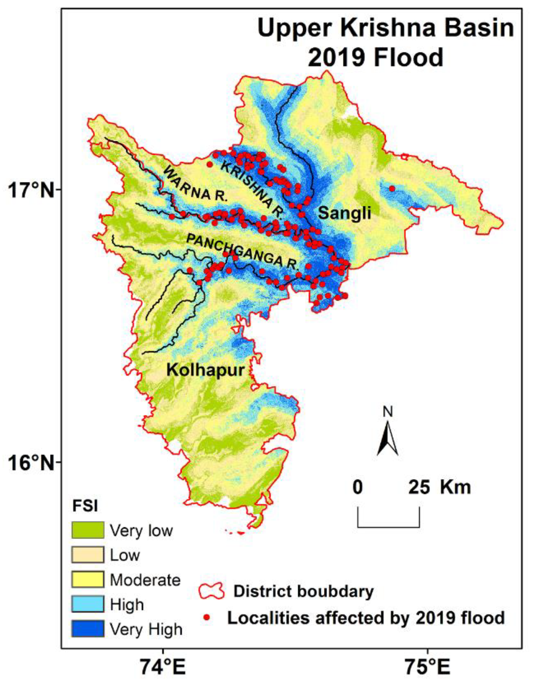
The UKB was severely affected by the disastrous flood in August 2019. Many parts of the Satara, Sangli, and Kolhapur districts in (Maharashtra), and the Belagavi, Bagalkote, and Vijaypura districts (Karnataka) were affected by the flood. The UKB received heavy rainfall from 27 July 2019 to 13 August 2019. Some of the stations located in the UKB recorded nearly 600% (Koyna, Mahabaleshwar) to 1500% (Sangli and Kolhapur) excess rainfall against average normal rain between 27 July and 13 August 2019 (18 days) [52]. Consequently, during a short period, an enormous discharge was produced by the major rivers (Krishna, Warna, and Panchganga) in the Satara, Sangli, and Kolhapur districts in Maharashtra (refer to Figure 7). The Krishna River, Warna River, and Panchganga River in the Sangli and Kolhapur districts became severely flooded on 5–6 August 2019. Extensive inundation in many parts of the Sangli and Kolhapur districts during the August 2019 flood was observed (refer to Figure 8). In the Sangli district, 58 villages covering about 15.17% of the area were affected. In Kolhapur district, 215 villages covering 21.20% of the area were affected [52]. In Sangli and Kolhapur districts, more than one lakh people from 20,000 families were moved to safety by the local people and the National Disaster Response Force (NDRF). About 29 boats in Kolhapur, 43 in Sangli, and 17 boats in Satara were busy evacuating people. In the Kolhapur district, 89 roads were underwater [91]. According to the Vadnere committee report [52], about 1.66 lakh hectares of seasonal and perennial crops were affected in 28 tehsils of Satara, Sangli, and Kolhapur districts. The estimated losses were Rs 3475 crores in these districts [52]. Figure 7 shows that most of the settlements are in the very-high-flood-susceptibility area of the UKB. Therefore, the present study is more beneficial to minimize the losses of infrastructures and settlements, animal and agriculture, and loss of human and animal lives.

5. Conclusions

The FSM is an essential aspect to understand the scenario of the flood hazard, vulnerability, and risk in hazard management. Therefore, it is indispensable to create the most accurate and trustworthy FSM of the UKB for flood prevention, management, and mitigation. There are several models for flood susceptibility analysis, but FR and SI models have been most frequently used in flood modeling [37]. Accordingly, FR and SI models were used for flood modeling in the UKB, and the FSM was produced by coalescing all of the weight conditioning factors. The model validation outcomes from ROC-AUC denoted that the FSM generated from the SI model is more reliable as compared to the FR model. The prediction rate of the SI model (83.23%) was greater than the FR model (68%). Therefore, the flood prediction accuracy and superior performance of the SI model are higher than the FR model. The FSM maps obtained for the UKB can be significantly supportive in understanding flood risks, flood possibilities, and flood preparedness to minimize the disastrous effects of floods in the UKB.

Author Contributions

Conceptualization, U.P. and U.R.; methodology, U.P. and W.S.; software, U.P. and W.S.; validation, U.P. and W.S.; formal analysis, U.P. and W.S.; investigation, U.P. and W.S.; resources, U.P.; data curation, U.P.; writing—original draft preparation, U.P. and W.S.; writing—review and editing, U.R. and N.M.; visualization, U.P. and W.S.; supervision, U.R.; project administration, U.R. All authors have read and agreed to the published version of the manuscript.

Funding

This research received no external funding.

Data Availability Statement

Data used in this analysis can be requested from the corresponding author for noncommercial and research purposes.

Conflicts of Interest

The authors declare no conflict of interest.

References

  1. Youssef, A.M.; Pradhan, B.; Hassan, A.M. Flash flood risk estimation along the St. Katherine road, southern Sinai, Egypt using GIS based morphometry and satellite imagery. Environ. Earth Sci. 2011, 62, 611–623. [Google Scholar] [CrossRef]
  2. Du, J.; Fang, J.; Xu, W.; Shi, P. Analysis of dry/wet conditions using the standardized precipitation index and its potential usefulness for drought/flood monitoring in Hunan Province China. Stoch. Environ. Res. Risk Assess. 2013, 27, 377–387. [Google Scholar] [CrossRef]
  3. Yu, J.; Qin, X.; Larsen, O. Joint Monte Carlo and possibilistic simulation for flood damage assessment. Stoch. Environ. Res. Risk Assess. 2013, 27, 725–735. [Google Scholar] [CrossRef]
  4. Zou, Q.; Zhou, J.; Zhou, C.; Song, L.; Guo, J. Comprehensive flood risk assessment based on set pair analysis-variable fuzzy sets model and fuzzy AHP. Stoch. Environ. Res. Risk Assess. 2013, 27, 525–546. [Google Scholar] [CrossRef]
  5. Tehrany, M.S.; Shabani, F.; Jebur, M.N.; Hong, H.; Chen, W.; Xie, X. GIS-based spatial prediction of flood prone areas using standalone frequency ratio, logistic regression, weight of evidence and their ensemble techniques. Geomatics. Nat. Hazards Risk 2017, 8, 1538–1561. [Google Scholar] [CrossRef] [Green Version]
  6. Pawar, U.V. An Analytical Study of Geomorphological, Hydrological, and Meteorological Characteristics of Floods in the Mahi River Basin: Western India. Ph.D. Thesis, Tilak Maharashtra Vidyapeeth, Pune, India, 2019. [Google Scholar]
  7. Toduse, N.C.; Ungurean, C.; Davidescu, S.; Clinciu, I.; Marin, M.; Nita, M.D.; Davidescu, A. Torrential flood risk assessment and environmentally friendly solutions for small catchments located in the Romania Natura 2000 sites Ciucas, Postavaru and Mare. Sci. Total Environ. 2020, 698, 134271. [Google Scholar] [CrossRef]
  8. Kazakis, N.; Kougias, I.; Patsialis, T. Assessment of flood hazard areas at a regional scale using an index-based approach and Analytical Hierarchy Process: Application in Rhodope-Evros region, Greece. Sci. Total Environ. 2015, 538, 555–563. [Google Scholar] [CrossRef]
  9. Wang, Y.; Hong, H.; Chen, W.; Li, S.; Panahi, M.; Khosravi, K.; Shirzadi, A.; Shahabi, H.; Panahi, S.; Costache, R. Flood susceptibility mapping in Dingnan County (China) using adaptive neuro-fuzzy inference system with biogeography based optimization and imperialistic competitive algorithm. J. Environ. Manag. 2019, 247, 712–729. [Google Scholar] [CrossRef]
  10. Charlton, R.; Fealy, R.; Moore, S.; Sweeney, J.; Murphy, C. Assessing the impact of climate change on water supply and flood hazard in Ireland using statistical downscaling and hydrological modeling techniques. Clim. Chang. 2006, 74, 475–491. [Google Scholar] [CrossRef]
  11. Pawar, U.V.; Hire, P.S.; Gunjal, R.P.; Patil, A.D. Modeling of magnitude and frequency of floods on the Narmada River: India. Modeling Earth Syst. Environ. 2020, 6, 2505–2516. [Google Scholar] [CrossRef]
  12. Alfieri, L.; Bisselink, B.; Dottori, F.; Naumann, G.; de Roo, A.; Salamon, P.; Wyser, K.; Feyen, L. Global projections of river flood risk in a warmer world. Earth’s Future 2017, 5, 171–182. [Google Scholar] [CrossRef]
  13. Pradhan, B. Flood susceptible mapping and risk area delineation using logistic regression, GIS and remote sensing. J. Spat. Hydrol. 2010, 9, 1–18. [Google Scholar]
  14. Diakakis, M.; Mavroulis, S.; Deligiannakis, G. Floods in Greece: A statistical and spatial approach. Nat. Hazards 2012, 62, 485–500. [Google Scholar] [CrossRef]
  15. Huang, X.; Tan, H.; Zhou, J.; Yang, T.; Benjamin, A.; Wen, S.W.; Li, S.; Liu, A.; Li, X.; Fen, S.; et al. Flood hazard in Hunan province of China: An economic loss analysis. Nat. Hazards 2008, 47, 65–73. [Google Scholar] [CrossRef]
  16. Dawson, C.W.; Abrahart, R.J.; Shamseldin, A.Y.; Wilby, R.L. Flood estimation at ungauged sites using artificial neural networks. J. Hydrol. 2006, 319, 391–409. [Google Scholar] [CrossRef] [Green Version]
  17. Bubeck, P.; Botzen, W.; Aerts, J. A review of risk perceptions and other factors that influence flood mitigation behavior. Risk Anal. 2012, 32, 1481–1495. [Google Scholar] [CrossRef] [Green Version]
  18. Mandal, S.P.; Chakrabarty, A. Flash flood risk assessment for upper Teesta river basin: Using the hydrological modeling system (HEC-HMS) software. Model. Earth Syst. Environ. 2016, 2, 59. [Google Scholar] [CrossRef] [Green Version]
  19. Bui, D.T.; Ngo, P.T.T.; Pham, T.D.; Jaafari, A.; Minh, N.Q.; Hoa, P.V.; Samui, P. A novel hybrid approach based on a swarm intelligence optimized extreme learning machine for flash flood susceptibility mapping. Catena 2019, 179, 184–196. [Google Scholar] [CrossRef]
  20. Bates, P.D. Remote sensing and flood inundation modeling. Hydrol. Process. 2004, 18, 2593–2597. [Google Scholar] [CrossRef]
  21. Liu, J.F.; Li, J.; Liu, J.; Cao, R.Y. Integrated GIS/AHP-based flood risk assessment: A case study of Huaihe River Basin in China. J. Nat. Disasters 2008, 17, 110–114. [Google Scholar]
  22. Haq, M.; Akhtar, M.; Muhammad, S.; Paras, S.; Rahmatullah, J. Techniques of Remote Sensing and GIS for flood monitoring and damage assessment: A case study of Sindh Province, Pakistan. Egypt. J. Remote Sens. Space Sci. 2012, 15, 135–141. [Google Scholar] [CrossRef] [Green Version]
  23. Jaafari, A.; Najafi, A.; Pourghasemi, H.; Rezaeian, J.; Sattarian, A. GIS-based frequency ratio and index of entropy models for landslide susceptibility assessment in the Caspian forest, Northern Iran. Int. J. Environ. Sci. Technol. 2014, 11, 909–926. [Google Scholar] [CrossRef]
  24. Rahmati, O.; Zeinivand, H.; Besharat, M. Flood hazard zoning in Yasooj region, Iran, using GIS and multi criteria decision analysis. Geomat. Nat. Hazards Risk 2016, 7, 1000–1017. [Google Scholar] [CrossRef] [Green Version]
  25. Paul, G.C.; Saha, S.; Hembram, T.K. Application of the GIS-based probabilistic models for mapping the flood susceptibility in Bansloi sub-basin of Ganga-Bhagirathi river and their comparison. Remote Sens. Earth Syst. Sci. 2019, 2, 120–146. [Google Scholar] [CrossRef]
  26. Msabi, M.M.; Makonyo, M. Flood susceptibility mapping using GIS and multi-criteria decision analysis: A case of Dodoma region, central Tanzania. Remote Sens. Appl. Soc. Environ. 2021, 21, 100445. [Google Scholar] [CrossRef]
  27. Suppawimut, W. GIS-Based Flood Susceptibility Mapping Using Statistical Index and Weighting Factor Models. Environ. Nat. Resour. 2021, 19, 481–493. [Google Scholar] [CrossRef]
  28. Malczewski, J. GIS-based multicriteria decision analysis: A survey of the literature. Int. J. Geograph. Inform. Sci. 2006, 20, 703–726. [Google Scholar] [CrossRef]
  29. Hwang, C.L.; Lin, M.J. Group Decision Making under Multiple Criteria: Methods and Applications; Springer: Berlin/Heidelberg, Germany, 2012. [Google Scholar]
  30. Sarker, S.; Veremyev, A.; Boginski, V.; Singh, A. Critical nodes in river networks. Sci. Rep. 2019, 9, 11178. [Google Scholar] [CrossRef] [Green Version]
  31. Gao, Y.; Sarker, S.; Sarker, T.; Leta, O.T. Analyzing the critical locations in response of constructed and planned dams on the Mekong River Basin for environmental integrity. Environ. Res. Commun. 2022, 4, 101001. [Google Scholar] [CrossRef]
  32. Talei, A.; Chua, L.H.C.; Quek, C. A novel application of a neurofuzzy computational technique in event-based rainfall–runoff modeling. Expert Syst. Appl. 2010, 37, 7456–7468. [Google Scholar] [CrossRef]
  33. Kia, M.B.; Pirasteh, S.; Pradhan, B.; Mahmud, A.R.; Sulaiman, W.N.A.; Moradi, A. An artificial neural network model for flood simulation using GIS: Johor River Basin Malaysia. Environ. Earth Sci. 2012, 67, 251–264. [Google Scholar] [CrossRef]
  34. Cao, C.; Xu, P.; Wang, Y.; Chen, J.; Zheng, L.; Niu, C. Flash flood hazard susceptibility mapping using frequency ratio and statistical index methods in coalmine subsidence areas. Sustainability 2016, 8, 948. [Google Scholar] [CrossRef]
  35. Khosravi, K.; Pourghasemi, H.R.; Chapi, K.; Bahri, M. Flash flood susceptibility analysis and its mapping using different bivariate models in Iran: A comparison between Shannon’s entropy, statistical index, and weighting factor models. Environ. Monit. Assess. 2016, 188, 656. [Google Scholar] [CrossRef]
  36. Samanta, S.; Pal, D.K.; Palsamanta, B. Flood susceptibility analysis through remote sensing, GIS and frequency ratio model. Appl. Water Sci. 2018, 8, 66. [Google Scholar] [CrossRef] [Green Version]
  37. Tehrany, M.S.; Kumar, L.; Jebur, M.N.; Shabani, F. Evaluating the application of the statistical index method in flood susceptibility mapping and its comparison with frequency ratio and logistic regression methods. Geomat. Nat. Hazards Risk 2019, 10, 79–101. [Google Scholar] [CrossRef] [Green Version]
  38. Hoang, D.V.; Tran, H.T.; Nguyen, T.T. A GIS-based spatial multi-criteria approach for flash flood risk assessment in the Ngan Sau-Ngan Pho mountainous river basin, North Central of Vietnam. Environ. Nat. Resour. J. 2020, 18, 110–123. [Google Scholar] [CrossRef] [Green Version]
  39. Khaing, T.W.; Tantanee, S.; Pratoomchai, W.; Mahavik, N. Coupling flood hazard with vulnerability map for flood risk assessment: A case study of Nyaung-U Township in Myanmar. GMSARN Int. J. 2021, 15, 127–138. [Google Scholar]
  40. Şen, Z. Flood Modelling, Predication and Mitigation; Springer International Publishing: Cham, Switzerland, 2018. [Google Scholar] [CrossRef]
  41. Shrestha, R.R.; Nestmann, F. Physically based and data-driven models and propagation of input uncertainties in river flood prediction. J. Hydrol. Eng. 2009, 14, 1309–1319. [Google Scholar] [CrossRef]
  42. Dhar, O.N.; Nandargi, S. Hydrometeorological aspects of floods in India. Nat. Hazards 2003, 28, 1–33. [Google Scholar] [CrossRef]
  43. Kale, V.S. Monsoon floods in India: A hydro-geomorphic perspective. Flood studies in India. Geol. Soc. India Mem. 1998, 41, 229–256. [Google Scholar]
  44. Hire, P.S. Geomorphic and Hydrologic studies of Floods in the Tapi Basin. Ph.D. Thesis, University of Pune, Pune, India, 2000. [Google Scholar]
  45. National Institution For Transforming India (NITI). Report of the Committee Constituted for Formulation of Strategy for Flood Management Works in Entire Country and River Management Activities and Works Related to Border Areas (2021–26); National Institution for Transforming: New Delhi, India, 2021. [Google Scholar]
  46. Naulin, J.P.; Payrastre, O.; Gaume, E. Spatially distributed flood forecasting in flash flood prone areas: Application to road network supervision in Southern France. J. Hydrol. 2013, 486, 88–99. [Google Scholar] [CrossRef] [Green Version]
  47. Guo, E.; Zhang, J.; Ren, X.; Zhang, Q.; Sun, Z. Integrated risk assessment of flood disaster based on improved set pair analysis and the variable fuzzy set theory in central Liaoning Province, China. Nat. Hazards 2014, 74, 947–965. [Google Scholar] [CrossRef]
  48. Ullah, K.; Zhang, J. GIS-based flood hazard mapping using relative frequency ratio method: A case study of Panjkora River Basin, eastern Hindu Kush, Pakistan. PLoS ONE 2020, 15, e0229153. [Google Scholar] [CrossRef] [PubMed]
  49. Chanapathi, T.; Thatikonda, S.; Raghavan, S. Analysis of rainfall extremes and water yield of Krishna river basin under future climate scenarios. J. Hydrol. Reg. Stud. 2018, 19, 287–306. [Google Scholar] [CrossRef]
  50. Rakhecha, P.R.; Deshpande, N.R.; Kulkarni, A.K.; Mandal, B.N.; Sangam, R.B. Design Storm Studies for the Upper Krishna River Catchment Upstream of the Almatti dam site. Theor. Appl. Climatol. 1995, 52, 219–229. [Google Scholar] [CrossRef]
  51. WRD. Integrated State Water Plan for Upper Krishna (k-1) Sub-Basin; WRD: Maharashtra, India, 2015; pp. 1–519. [Google Scholar]
  52. GOM. Expert Study Committee Report: Floods 2019 (Krishna Basin); GOM: Maharashtra, India, 2020; pp. 1–190. [Google Scholar]
  53. GOK. Seeking Central Assistance for Relief and Emergency Works Due to Flood and Landslides in Karnataka during August 2019. In Memorandum; GOK: Karnataka, India, 2019; pp. 1–209. [Google Scholar]
  54. Ali, S.A.; Khatun, R.; Ahmad, A.; Ahmad, S.N. Application of GIS-based analytic hierarchy process and frequency ratio model to flood vulnerable mapping and risk area estimation at Sundarban region, India. Model. Earth Syst. Environ. 2019, 5, 1083–1102. [Google Scholar] [CrossRef]
  55. Chowdhuri, I.; Pal, S.; Chakrabortty, R. Flood susceptibility mapping by ensemble evidential belief function and binomial logistic regression model on river basin of eastern India. Adv. Space Res. 2020, 65, 1466–1489. [Google Scholar] [CrossRef]
  56. Vafakhah, M.; Mohammad Hasani Loor, S.; Pourghasemi, H.; Katebikord, A. Comparing performance of random forest and adaptive neuro-fuzzy inference system data mining models for flood susceptibility mapping. Arabian J. Geosci 2020, 13, 11. [Google Scholar] [CrossRef]
  57. Mahato, S.; Pal, S.; Talukdar, S.; Saha, T.; Mandal, P. Field based index of flood vulnerability (IFV): A new validation technique for flood susceptible models. Geosci. Front. 2021, 12, 101175. [Google Scholar] [CrossRef]
  58. Hasanuzzaman, M.; Adhikary, P.; Bera, B.; Shit, P. Flood vulnerability assessment using AHP and frequency ratio techniques. In Spatial Modelling of Flood Risk and Flood Hazards; Springer Nature: Cham, Switzerland, 2022; p. 91. [Google Scholar] [CrossRef]
  59. Pradhan, B.; Tehrany, M.S.; Jebur, M.N. A new semi-automated detection mapping of flood extent from TerraSAR-X satellite image using rule-based classification and Taguchi optimization techniques. IEEE Trans. Geosci. Remote Sens. 2016, 54, 4331–4342. [Google Scholar] [CrossRef]
  60. Nguyen, V.N.; Yariyan, P.; Amiri, M.; Dang Tran, A.; Pham, T.D.; Do, M.P.; Tien Bui, D. A new modeling approach for spatial prediction of flash flood with biogeography optimized CHAID tree ensemble and remote sensing data. Remote Sens. 2020, 12, 1373. [Google Scholar] [CrossRef]
  61. Souissi, D.; Zouhri, L.; Hammami, S.; Msaddek, M.H.; Zghibi, A.; Dlala, M. GIS-based MCDM–AHP modeling for flood susceptibility mapping of arid areas, Southeastern Tunisia. Geocarto Int. 2020, 35, 991–1017. [Google Scholar] [CrossRef]
  62. Bathrellos, G.D.; Skilodimou, H.D.; Soukis, K.; Koskeridou, E. Temporal and spatial analysis of flood occurrences in the drainage basin of Pinios river (Thessaly, Central Greece). Land 2018, 7, 106. [Google Scholar] [CrossRef] [Green Version]
  63. Young, R.A.; Mutchler, C.K. Effect of slope shape on erosion and runoff. Trans. ASAE 1969, 12, 0231–0233. [Google Scholar] [CrossRef]
  64. Hudson, P.F.; Kesel, R.H. Channel migration and meander-bend curvature in the lower Mississippi River prior to major human modification. Geology 2000, 28, 531–534. [Google Scholar] [CrossRef]
  65. Qin, C.Z.; Zhu, A.X.; Pei, T.; Li, B.L.; Scholten, T.; Behrens, T.; Zhou, C.H. An approach to computing topographic wetness index based on maximum downslope gradient. Precis. Agric. 2011, 12, 32–43. [Google Scholar] [CrossRef]
  66. Jebur, M.N.; Pradhan, B.; Tehrany, M.S. Optimization of landslide conditioning factors using very high-resolution airborne laser scanning (LiDAR) data at catchment scale. Remote Sens. Environ. 2014, 152, 150–165. [Google Scholar] [CrossRef]
  67. Patil, A.D.; Hire, P.S. Flood hydrometeorological situations associated with monsoon floods on the Par River in western India. Mausam 2021, 71, 687–698. [Google Scholar]
  68. Pawar, U.; Rathnayake, U. Spatiotemporal rainfall variability and trend analysis over Mahaweli Basin, Sri Lanka. Arab. J. Geosci. 2022, 15, 370–416. [Google Scholar] [CrossRef]
  69. Pawar, U.; Karunathilaka, P.; Rathnayake, U. Spatio-Temporal Rainfall Variability and Concentration over Sri Lanka. Adv. Meteorol. 2022, 2022, 6456761. [Google Scholar] [CrossRef]
  70. Shekhar, S.; Pandey, A.C. Delineation of groundwater potential zone in hard rock terrain of India using remote sensing, geographical information system (GIS) and analytic hierarchy process (AHP) techniques. Geocarto. Int. 2015, 30, 402–421. [Google Scholar] [CrossRef]
  71. Capon, S.J. Flood variability and spatial variation in plant community composition and structure on a large arid floodplain. J. Arid. Environ. 2005, 60, 283–302. [Google Scholar] [CrossRef]
  72. Chaplot, V.; Poesen, J. Sediment, soil organic carbon and runoff delivery at various spatial scales. Catena 2012, 88, 46–56. [Google Scholar] [CrossRef]
  73. Hölting, B.; Coldewey, W.G. Surface water infiltration. In Hydrogeology; Springer: Berlin/Heidelberg, Germany, 2019; pp. 33–37. [Google Scholar]
  74. Chen, Y.; Liu, R.; Barrett, D.; Gao, L.; Zhou, M.; Renzullo, L.; Emelyanova, I. A spatial assessment framework for evaluating flood risk under extreme climates. Sci. Total Environ. 2015, 538, 512–523. [Google Scholar] [CrossRef]
  75. Youssef, A.M.; Pradhan, B.; Sefry, S.A. Flash flood susceptibility assessment in Jeddah city (Kingdom of Saudi Arabia) using bivariate and multivariate statistical models. Environ. Earth Sci. 2016, 75, 1–16. [Google Scholar] [CrossRef]
  76. Hammami, S.; Zouhri, L.; Souissi, D.; Souei, A.; Zghibi, A. Application of the GIS based multi-criteria decision analysis and analytical hierarchy process (AHP) in the flood susceptibility mapping (Tunisia). Arab. J. Geosci. 2019, 12, 653. [Google Scholar] [CrossRef]
  77. Roslee, R.; Tongkul, F.; Mariappan, S.; Simon, N. Flood hazard analysis (FHAn) using multi-criteria evaluation (MCE) in Penampang Area, Sabah Malaysia. ASM Sci. J. 2018, 11, 104–122. [Google Scholar]
  78. Yalcin, A.; Reis, S.; Aydinoglu, A.C.; Yomralioglu, T. A GIS-based comparative study of frequency ratio, analytical hierarchy process, bivariate statistics and logistic regression methods for landslide susceptibility mapping in Trabzon, NE Turkey. Catena 2011, 85, 274–287. [Google Scholar] [CrossRef]
  79. Wu, Y.; Li, W.; Wang, Q.; Liu, Q.; Yang, D.; Xing, M.; Pei, Y.; Yan, S. Landslide Susceptibility Assessment Using Frequency Ratio, Statistical Index and Certainty Factor Models for the Gangu County, China. Arab. J. Geosci. 2016, 9, 84. [Google Scholar] [CrossRef]
  80. Tiwari, A.; Shoab, M.; Dixit, A. GIS-based forest fire susceptibility modeling in Pauri Garhwal, India: A comparative assessment of frequency ratio, analytic hierarchy process and fuzzy modeling techniques. Nat. Hazards 2021, 105, 1189–1230. [Google Scholar] [CrossRef]
  81. Rehman, A.; Song, J.; Haq, F.; Mahmood, S.; Ahamad, M.I.; Basharat, M.; Sajid, M.; Mehmood, M.S. Multi-Hazard Susceptibility Assessment Using the Analytical Hierarchy Process and Frequency Ratio Techniques in the Northwest Himalayas, Pakistan. Remote Sens. 2022, 14, 554. [Google Scholar] [CrossRef]
  82. Westen, C.J.V. Statistical Landslide Hazard Analysis. ILWIS 2.1 for Windows Application Guide; ITC Publication: Enschede, The Netherlands, 1997; pp. 73–84. [Google Scholar]
  83. Ali, S.A.; Parvin, F.; Pham, Q.B.; Vojtek, M.; Vojteková, J.; Costache, R.; Thuy Linh, N.T.; Nguyen, H.Q.; Ahmad, A.; Ghorbani, M.A. GIS-Based Comparative Assessment of Flood Susceptibility Mapping Using Hybrid Multi-Criteria Decision-Making Approach, Naïve Bayes Tree, Bivariate Statistics and Logistic Regression: A Case of Topla Basin, Slovakia. Ecol. Indic. 2020, 117, 106620. [Google Scholar] [CrossRef]
  84. Rossi, M.; Reichenbach, P. LAND-SE: Software for statistically based landslide susceptibility zonation, version 1.0. Geosci. Model. Dev. 2016, 9, 3533–3543. [Google Scholar] [CrossRef] [Green Version]
  85. Wahono, B.F.D. Applications of statistical and heuristic methods for landslide susceptibility assessments: A case study in Wadas Lintang Sub District, Wonosobo Regency, Central Java Province, Indonesia. Ph.D. Thesis, Gadjah Mada University, Sleman, Indonesia, 2010; pp. 12–37. [Google Scholar]
  86. Pimiento, E. Shallow landslide susceptibility: Modelling and validation. Ph.D. Thesis, Lund University, Lund, Sweden, 2010; pp. 25–29. [Google Scholar]
  87. Silalahi, F.E.S.; Pamela; Arifianti, Y.; Hidayat, F. Landslide susceptibility assessment using frequency ratio model in Bogor, West Java, Indonesia. Geosci. Lett. 2019, 6, 10. [Google Scholar] [CrossRef]
  88. Jaiswal, R.K.; Mukherjee, S.; Krishnamurthy, J.; Saxena, R. Role of remote sensing and GIS techniques for generation of groundwater prospect zones towards rural development—An approach. Int. J. Remote Sens. 2003, 24, 993–1008. [Google Scholar] [CrossRef]
  89. Sharif, H.O.; Al-Juaidi, F.H.; Al-Othman, A.; Al-Dousary, I.; Fadda, E.; Jamal-Uddeen, S.; Elhassan, A. Flood hazards in an urbanizing watershed in Riyadh, Saudi Arabia. Geomat. Nat. Hazards Risk 2016, 7, 702–720. [Google Scholar] [CrossRef] [Green Version]
  90. Dudal, R. Dark Clay Soils of Tropical and Subtropical Regions; FAO Agricultural Development Paper No. 83; FAO: Rome, Italy, 1965. [Google Scholar]
  91. De Vos, J.H.; Virgo, K.J. Soil structure in vertisols of the Blue Nile clay plains, Sudan. Eur. J. Soil Sci. 1969, 20, 189–206. Available online: https://www.thehindu.com/news/national/other-states/floods-paralyse-kolhapur-sangli-132-lakh-evacuated/article28873771.ece (accessed on 27 October 2022). [CrossRef]
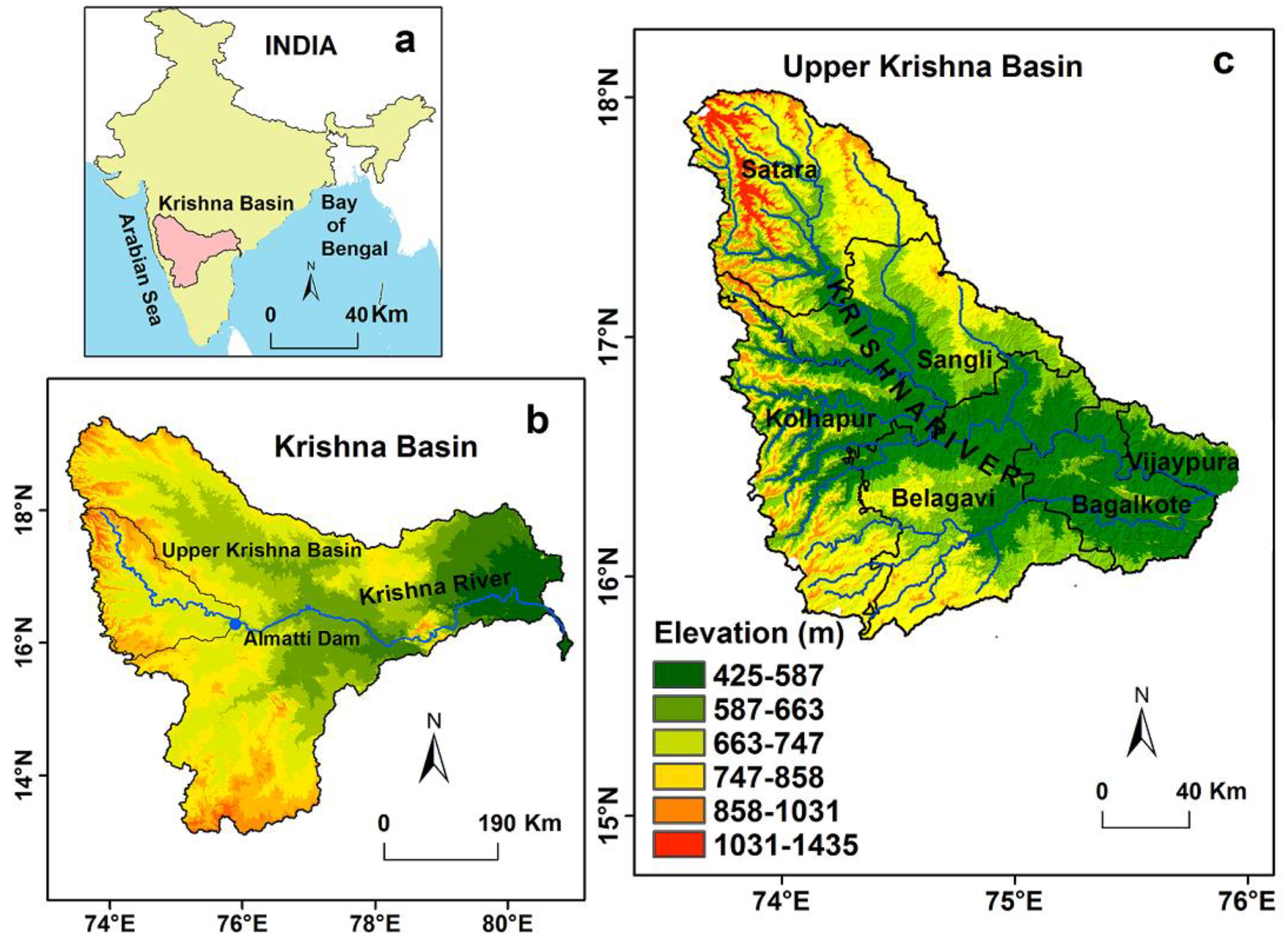
Figure 1. Study area: (a) India; (b) Krishna Basin; (c) Upper Krishna Basin.
Water 14 03771 g001
Figure 2. Flow chart of the research methodology.
Water 14 03771 g002
Figure 3. Flood locations in the UKB (August 2019).
Water 14 03771 g003
Figure 4. Flood controlling factors used for flood susceptibility analysis.
Water 14 03771 g004
Figure 5. Flood susceptibility maps of UKB: (a) based on FR; (b) based on SI models.
Water 14 03771 g005
Figure 6. ROC curves of success and prediction rates of the FR and SI models.
Water 14 03771 g006
Figure 7. Severely flood-affected areas in Sangli and Kolhapur districts (August 2019).
Water 14 03771 g007
Figure 8. Clips of 2019 flood in the UKB: (a) A view of flooded areas due to overflowing Panchganga River in Kolhapur city (Maharashtra) on 7 August 2019 (PTI). Source: Shivam Bodhe/HT photo. Accessed from: http://www.hindustantimes.com on 27 October 2022; (b) a view of flooded areas due to overflowing Krishna River in Sangli on 6–7 August 2019 (PTI). Accessed from: http://indianexpress.com/article on 27 October 2022.
Water 14 03771 g008
Table 1. Parameters used for flood susceptibility mapping, their sources, and descriptions.
Flood Conditioning
Factors
Data TypeDescriptionsSource
ElevationRaster gridDerived from ASTER DEM (30 m × 30 m) using ArcGISUSGS
https://earthexplorer.usgs.gov (accessed on 23 August 2022)
Slope
Aspect
Curvature
TWI
SPI
RainfallAttribute dataDerived from raingauge rainfall data and converted into raster data with 30 m × 30 m cell sizeDepartment of Agriculture, Maharashtra, India Meteorological Department, and Karnataka Sate Natural Disaster Monitoring Center, India
Distance from the riverVector data (Line)Derived from stream networks of the UKB (30 m × 30 m) using ArcGISUSGS
https://earthexplorer.usgs.gov (accessed on 23 August 2022)
Stream densityRaster gridDerived from ASTER DEM (30 m × 30 m) using fill, flow
accumulation, drainage density command in ArcGIS
USGS https://earthexplorer.usgs.gov (accessed on 23 August 2022)
Soil typesVector data (Polygon)Digital soil map of the world-ESRI shape fileFAO http://www.fao.org (accessed on 22 August)
Land useRaster gridLandsat 8 OLI/TIRS, 30 m × 30 mUSGS https://earthexplorer.usgs.gov (accessed on 25 August 2022)
Distance from the roadVector data (Line)Derived from road networks of the district and converted into raster data with 30 m × 30 m cell sizeDIVA-GIS
https://www.diva-gis.org › gdata (accessed on 23 August 2022)
Flood inventory databaseVector data (Point)Google Earth and ReportsElectronic Media (News), Print Media (Newspaper), Social Media, and Published Reports
Table 2. Result of the FR and SI model for different classes of the factors.
FactorsClassNo. PixelsArea (%)Floods PixelsFlood (%)Frequency Ratio (FR)Stastical Index (SI)
Elevation (m)425–5871368598137.5822586.872.3184
587–663933158725.622810.810.42−86
663–747691856519.0051.930.10−229
747–858422101411.5910.390.03−340
858–103117033244.6800.000.000
1031–14355599061.5400.000.000
Slope
(degree)
0–3.051285959735.316926.640.75−28
3.05–6.651374117037.7313552.121.3832
6.65–11.35570377915.665019.311.2321
11.35–18.0123825276.5451.930.30−122
18.01–27.1412269793.3700.000.000
27.14–70.615063251.3900.000.000
AspectFlat398971710.95197.340.67−40
North731170220.082610.040.50−69
Northeast35892969.86259.650.98−2
East379436610.422710.421.000
Southeast413059811.343613.901.2320
South35684399.80259.650.99−1
Southwest36281619.964316.601.6751
West32747178.993212.361.3732
Northwest31333818.602610.041.1715
CurvatureConvex390348610.72166.180.58−55
Flat2085758357.2714656.370.98−2
Concave1165930832.019737.451.1716
Topographic Wetness Index
(TWI)
2.36–6.231147937231.5211745.171.4336
6.23–7.831393765538.2710640.931.077
7.83–9.81610742916.77259.650.58−55
9.81–12.4030139288.2872.700.33−112
12.40–15.9816042714.4041.540.35−105
15.98–27.712777220.7600.000.000
Stream Power Index
(SPI)
−13.82–−6.321534803542.1415961.391.4638
−6.32–−1.92534789114.683413.130.89−11
−1.92–−0.14826813322.704818.530.82−20
−0.14–2.00498970613.70135.020.37−100
2.00–5.2120275535.5751.930.35−106
5.21–16.514390591.2100.000.000
Rainfall (mm)470–8261699850046.6715559.851.2825
826–1267998578627.428532.821.2018
1267–1875662100818.18197.340.40−91
1875–273617597034.8300.000.000
2736–40377779592.1400.000.000
4037–58212774210.7600.000.000
Distance from rivers (m)0–22821049475028.8222687.263.03111
2282–4979960965826.392710.420.40−93
4979–7884792730421.7731.160.05−293
7884–11,411497305213.6520.770.06−287
11,411–15,76825845437.1010.390.050
15,768–26,3498310702.2800.000.000
Stream density
(km/sq.km)
0.05–0.39559465215.3620.770.05−299
0.39–0.57941460425.8531.160.04−311
0.57–0.73769310921.12135.020.24−144
0.73–0.92656615518.035521.241.1816
0.92–1.13471954712.969536.682.83104
1.13–1.5824323106.689135.145.26166
Soil TypesAp552750015.1893.470.23−147
Bv19439255.3410.390.07−263
Hh31726248.713513.511.5544
l288520.0800.000.000
Lc24682826.7810.390.06−287
Nd396355510.8862.320.21−155
Ne1203720.3300.000.000
Vc1525197041.8812949.811.1917
Vp394329710.837830.122.78102
Land useAgriculture1417093038.915119.690.51−68
Built-up/Urban14316233.9313652.5113.36259
Forest25614317.0300.000.000
Open Land1029551328.276223.940.85−17
Shrub Land709623619.49103.860.20−162
Water Bodies8631842.3700.000.000
Distance from road (m)0–12861258133134.5410139.001.1312
1286–29161118841230.729235.521.1615
2916–4804717418319.704316.600.84−17
4804–7291382314710.50207.720.74−31
7291–11,23813292143.6531.160.32−115
11,238–21,8753240900.8900.000.000
Publisher’s Note: MDPI stays neutral with regard to jurisdictional claims in published maps and institutional affiliations.