
Comparison of Three-Parameter Distributions in Controlled Catchments for a Stationary and Non-Stationary Data Series

 , ,
, ,  ,
,
Abstract
:1. Introduction
2. Materials and Methods
2.1. Study Area
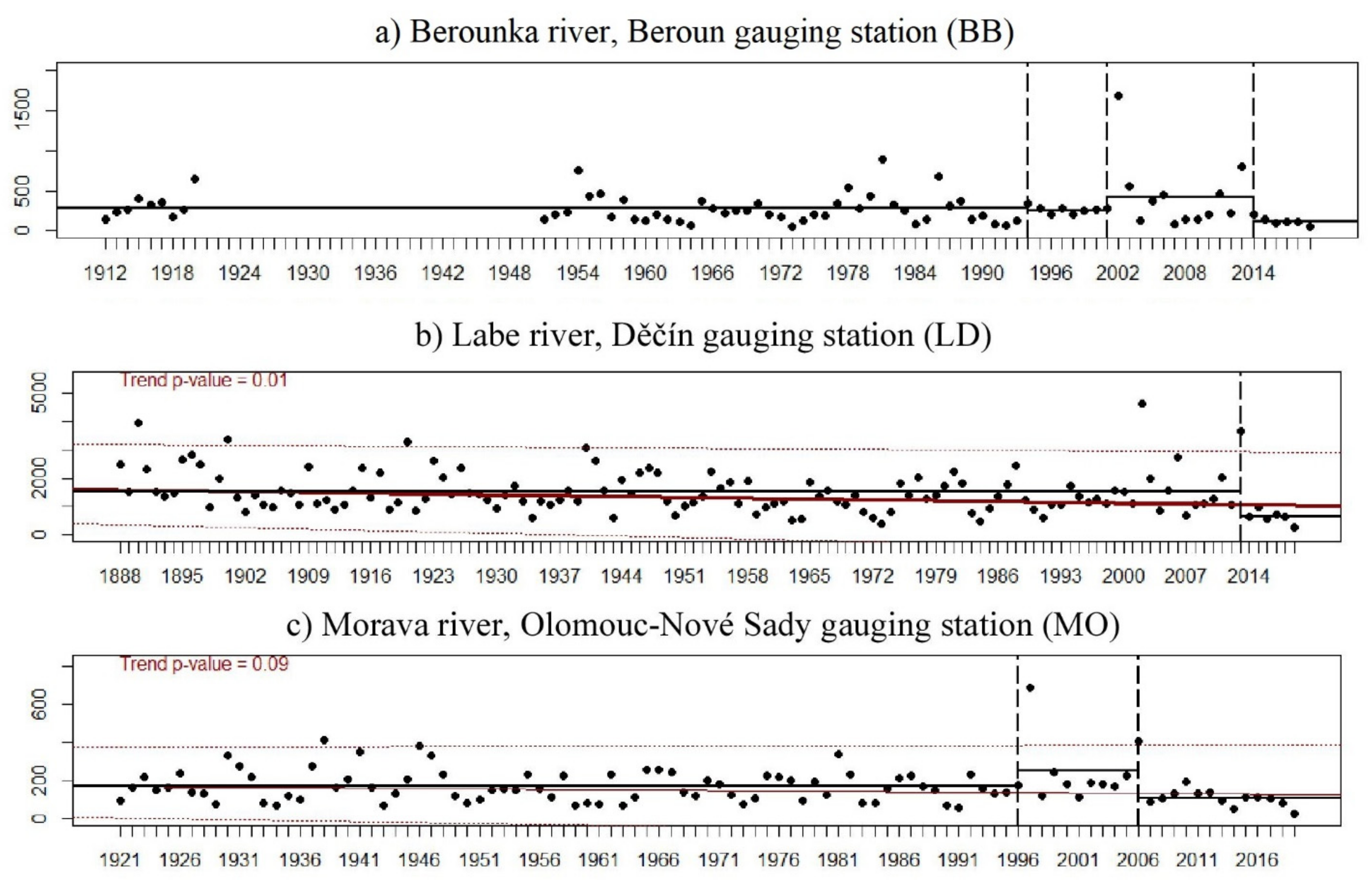
2.2. Change Point Analysis
2.3. Temporal Trend Analysis
2.4. Test for Randomness
2.5. PDF Fitting by the MLE
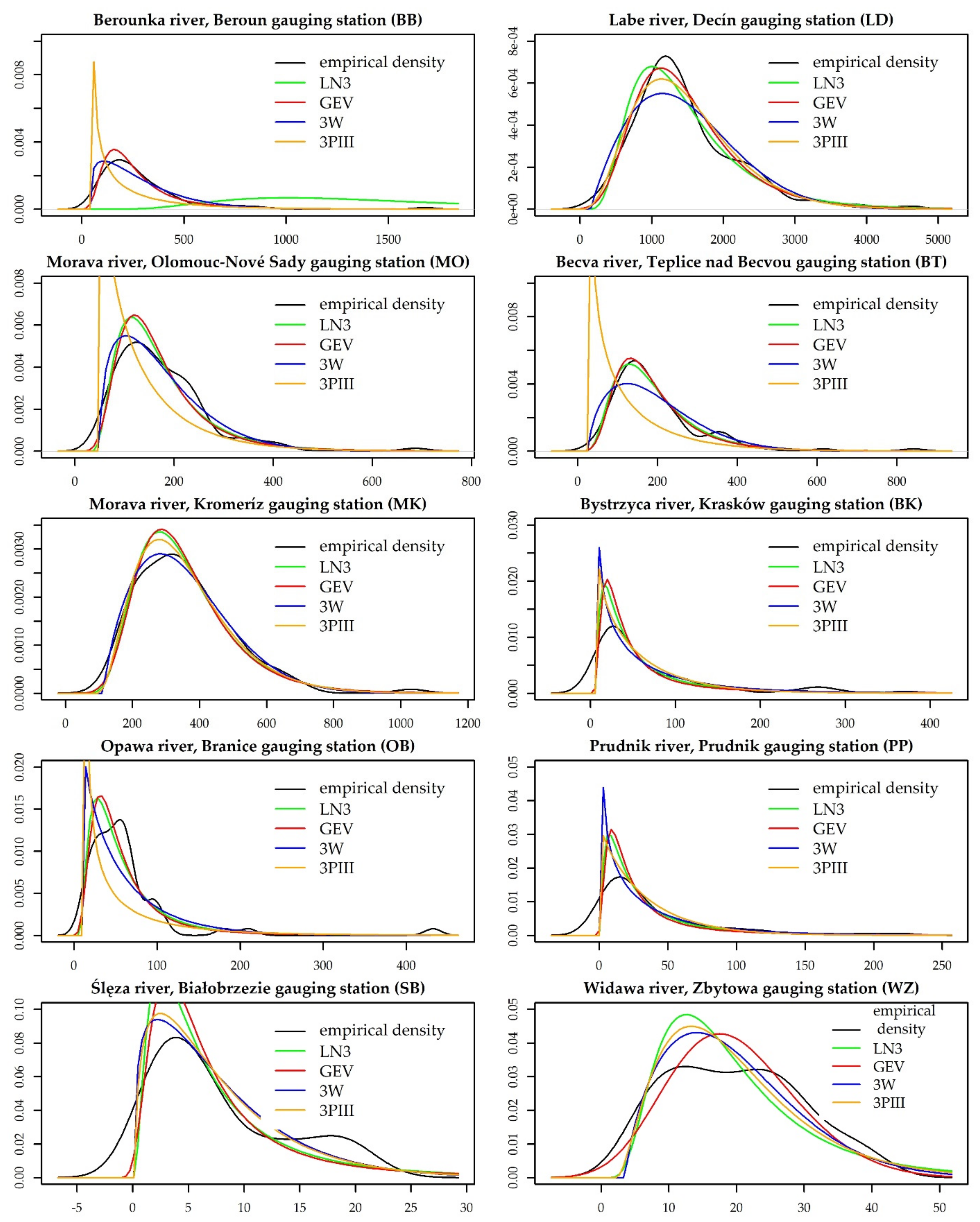
2.6. Probability Density Function (PDF)
2.7. The Goodness-of-Fit Tests (GOF Tests)
3. Results
4. Discussion
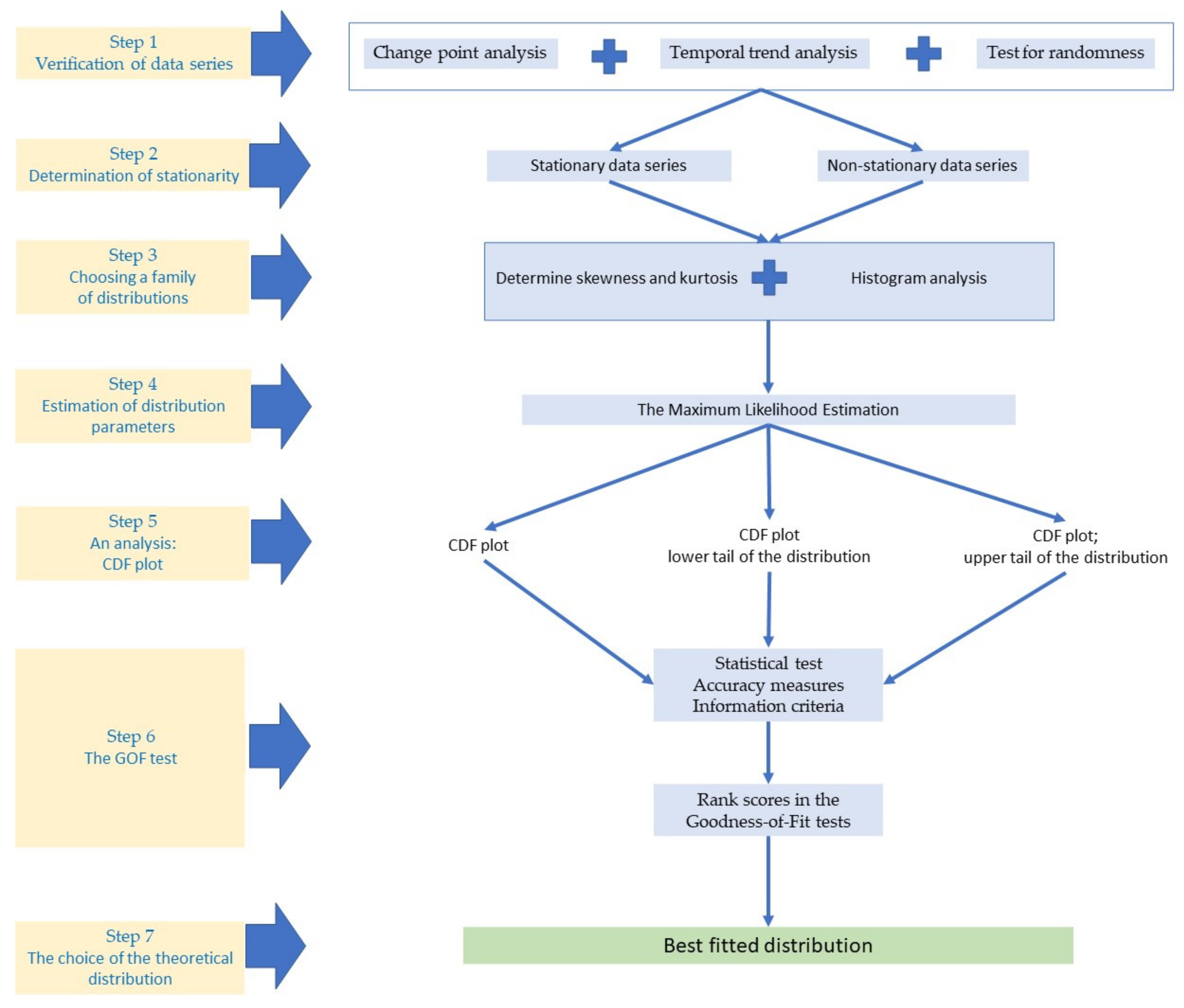
- Proposing to standardize the verification of data series before performing the FFA and non-stationary FFA procedures;
- Histograms of the empirical data series determine the family of the distributions; the use of histograms easily allows for such an assessment;
- The MLE method allows one to simplify the analysis whenever there is a series of data, both stationary and non-stationary;
- Combining the graphical method (CDF plot) and the analytical method (GOF test);
- Our results will find the optimal three-parameter distribution for a given data series in the upper and/or the lower tail.
5. Conclusions
Author Contributions
Funding
Data Availability Statement
Acknowledgments
Conflicts of Interest
Appendix A
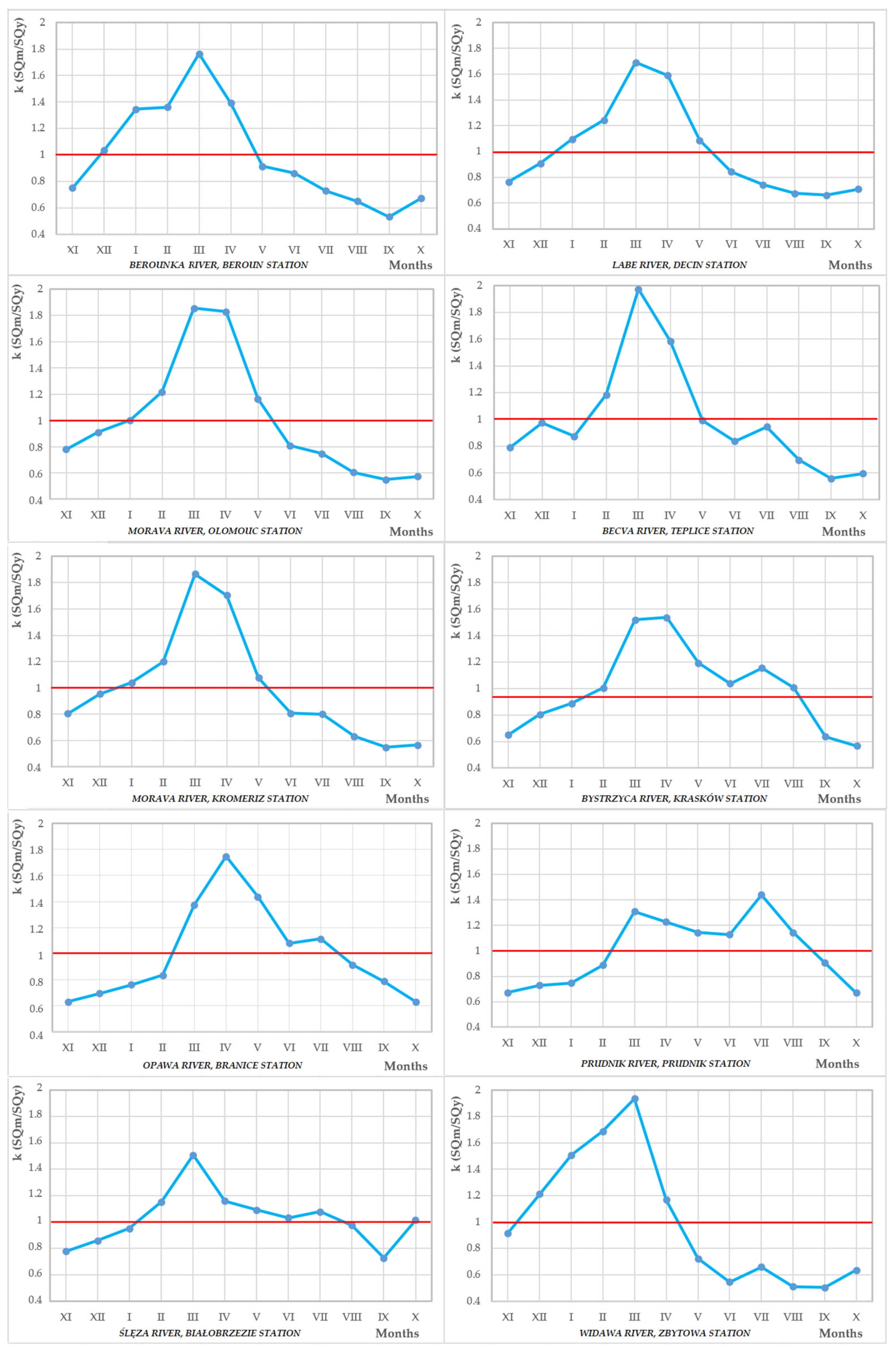

| River, Station | Kr | Cm | QmeanXII-V and Qmeany (Qmeana) | Regime–Parde | Regime–Dynowska |
|---|---|---|---|---|---|
| Berounka, Beroun | 3.80 (average balanced flows) | 36.53% (slightly unbalanced outflow) | QmeanXII-V > Qmeany (lowland and highland streams) | simple snow–rain, mountain variety | nival |
| Labe, Decin | 3.41 (average balanced flows) | 33.68% (slightly unbalanced outflow) | |||
| Morava, Olomouc | 4.10 (average balanced flows) | 42.76% (slightly unbalanced outflow) | |||
| Becva, Teplice | 3.47 (average balanced flows) | 39.40% (slightly unbalanced outflow) | |||
| Morava, Kromeriz | 3.78 (average balanced flows) | 40.16% (slightly unbalanced outflow) | |||
| Bystrzyca, Kraskow | 2.91 (very balanced alpine flows) | 30.5% (slightly unbalanced outflow) | QmeanXII-V > Qmeany (lowland and highland streams) | composite snow–rain regime | nival –pluvial |
| Opawa, Branice | 3.51 (average balanced flows) | 34.34% (slightly unbalanced outflow) | |||
| Prudnik, Prudnik | 2.79 (very balanced alpine flows) | 25.38% (balanced outflow) | QmeanXII-V < Qmeany (alpine streams) | pluvial –nival | |
| Sleza, Bialobrzezie | 1.68 (very balanced alpine flows) | 19.75% (balanced outflow) | QmeanXII-V > Qmeany (lowland and highland streams) | nival –pluvial | |
| Widawa, Zbytowa | 5.03 (average balanced flows) | 47.5% (slightly unbalanced outflow) | composite rain, oceanic variety | nival |
Appendix B
| Data Series | Distribution | AD Amax | AD p.Value | MARE | MAE | RMSE | AIC | BIC |
|---|---|---|---|---|---|---|---|---|
| BB | GEV | 1.05 | 0.972 | 3.81 | 15.09 | 61.74 | 995.4 | 1002.5 |
| LN3 | 1.53 | 0.812 | 4.15 | 18.20 | 75.80 | 995.7 | 1002.7 | |
| Weibull | 2.36 | 0.429 | 9.25 | 31.82 | 89.38 | 1002.9 | 1009.9 | |
| LD | GEV | 3.10 | 0.262 | 3.93 | 49.98 | 79.88 | 2107.5 | 2116.1 |
| LN3 | 3.93 | 0.112 | 4.62 | 45.20 | 61.23 | 2113.9 | 2122.6 | |
| Weibull | 2.18 | 0.604 | 7.22 | 92.04 | 141.40 | 2116.2 | 2124.9 | |
| PIII | 1.35 | 0.946 | 4.77 | 65.44 | 117.04 | 2110.1 | 2118.7 | |
| MO | GEV | 2.98 | 0.255 | 3.89 | 7.75 | 17.21 | 1129.6 | 1137.3 |
| Weibull | 2.48 | 0.413 | 3.40 | 7.74 | 24.60 | 1129.3 | 1137.1 | |
| BT | GEV | 1.69 | 0.773 | 4.92 | 11.08 | 29.58 | 1088.2 | 1095.8 |
| LN3 | 2.98 | 0.256 | 5.75 | 12.95 | 34.28 | 1090.8 | 1098.4 | |
| Weibull | 1.86 | 0.694 | 11.21 | 21.12 | 40.90 | 1104.8 | 1112.4 | |
| MK | GEV | 2.74 | 0.323 | 2.62 | 9.46 | 21.10 | 1300.2 | 1308.1 |
| LN3 | 2.33 | 0.473 | 2.50 | 9.13 | 21.35 | 1299.5 | 1307.4 | |
| Weibull | 1.92 | 0.664 | 2.26 | 8.66 | 26.85 | 1301.2 | 1309.1 | |
| PIII | 2.00 | 0.622 | 2.06 | 7.77 | 23.67 | 1299.2 | 1307.1 | |
| BK | GEV | 1.83 | 0.626 | 9.98 | 12.78 | 40.38 | 709.2 | 715.9 |
| Weibull | 2.25 | 0.435 | 13.20 | 8.36 | 15.69 | 706.5 | 713.2 | |
| OB | GEV | 2.52 | 0.302 | 9.54 | 9.48 | 30.28 | 488.4 | 494.0 |
| LN3 | 1.94 | 0.524 | 10.46 | 10.46 | 31.90 | 488.9 | 494.6 | |
| Weibull | 2.21 | 0.409 | 17.07 | 13.50 | 31.58 | 492.7 | 498.3 | |
| PP | GEV | 2.15 | 0.477 | 12.98 | 6.64 | 22.17 | 599.9 | 606.4 |
| LN3 | 2.14 | 0.483 | 10.59 | 3.59 | 6.33 | 597.1 | 603.6 | |
| Weibull | 3.16 | 0.175 | 11.05 | 3.61 | 7.01 | 593.9 | 600.4 | |
| SB | GEV | 3.33 | 0.146 | 13.44 | 1.32 | 3.10 | 416.1 | 422.8 |
| LN3 | 1.92 | 0.580 | 12.20 | 1.12 | 2.50 | 413.8 | 420.5 | |
| Weibull | 3.77 | 0.092 | 12.39 | 0.87 | 1.25 | 411.1 | 417.8 | |
| PIII | 1.13 | 0.939 | 12.01 | 0.87 | 1.33 | 411.1 | 417.8 | |
| WZ | LN3 | 1.53 | 0.729 | 9.63 | 1.87 | 2.87 | 366.9 | 372.6 |
| Weibull | 2.09 | 0.458 | 7.38 | 1.18 | 1.44 | 361.0 | 366.6 | |
| PIII | 1.50 | 0.744 | 7.68 | 1.37 | 1.86 | 363.5 | 369.2 |
References
- Seckin, N.; Yurtal, R.; Haktanir, T.; Dogan, A. Comparison of probability weighted moments and maximum likelihood methods used in flood frequency analysis for Ceyhan river basin. Arab. J. Sci. Eng. 2010, 35, 49. [Google Scholar]
- Khanal, S.; Ridder, N.; de Vries, H.; Terink, W.; van den Hurk, B. Storm Surge and Extreme River Discharge: A Compound Event Analysis Using Ensemble Impact Modeling. Front. Earth Sci. 2019, 7, 224. [Google Scholar] [CrossRef]
- Buchlák, J.; Matějka, J.; Ryjáček, P.; Bílý, P.; Procházka, J.; Pollert, J.; Fabel, J. Experimental verification of functionality of fibre-reinforced concrete submersible piers. IOP Conf. Ser. Mater. Sci. Eng. 2019, 596, 012029. [Google Scholar] [CrossRef]
- Hassan, M.U.; Hayat, O.; Noreen, Z. Selecting the best probability distribution for at-site flood frequency analysis, a study of Torne River. SN Appl. Sci. 2019, 1, 1629. [Google Scholar] [CrossRef] [Green Version]
- Langat, P.K.; Kumar, L.; Koech, R. Identification of the Most Suitable Probability Distribution Models for Maximum, Minimum, and Mean Streamflow. Water 2019, 11, 734. [Google Scholar] [CrossRef] [Green Version]
- Myronidis, D.; Stathis, D.; Sapountzis, M. Post-Evaluation of Flood Hazards Induced by Former Artificial Interventions along a Coastal Mediterranean Settlement. J. Hydrol. Eng. 2016, 21, 05016022. [Google Scholar] [CrossRef]
- Sweet, W.V.; Genz, A.S.; Obeysekera, J.; Marra, J.J. A Regional Frequency Analysis of Tide Gauges to Assess Pacific Coast Flood Risk. Front. Mar. Sci. 2020, 7, 581769. [Google Scholar] [CrossRef]
- Dunne, T.; Leopold, L.B. (Eds.) Calculation of flood hazard. In Water in Environmental Planning; W.H. Freeman: San Francisco, CA, USA, 1978; pp. 279–391. [Google Scholar]
- Alila, Y.; Mtiraoui, A. Implications of heterogeneous flood-frequency distributions on traditional stream-discharge prediction techniques. Hydrol. Process. 2002, 16, 1065–1084. [Google Scholar] [CrossRef]
- Katz, R.W.; Parlange, M.B.; Naveau, P. Statistics of extremes in hydrology. Adv. Water Resour. 2002, 25, 1287–1304. [Google Scholar] [CrossRef] [Green Version]
- Cassalho, F.; Beskow, S.; de Mello, C.R.; de Moura, M.M.; Kerstner, L.; Ávila, L.F. At-Site Flood Frequency Analysis Coupled with Multi-parameter Probability Distributions. Water Resour. Manag. 2018, 32, 285–300. [Google Scholar] [CrossRef]
- Młyński, D.; Petroselli, A.; Wałęga, A. Flood frequency analysis by an event-based rainfall–runoff model in selected catchments of southern Poland. Soil Water Res. 2018, 13, 170–176. [Google Scholar] [CrossRef] [Green Version]
- Szulczewski, W.; Jakubowski, W. The Application of Mixture Distribution for the Estimation of Extreme Floods in Controlled Catchment Basins. Water Resour. Manag. 2018, 32, 3519–3534. [Google Scholar] [CrossRef] [Green Version]
- Myronidis, D.; Ivanova, E. Generating Regional Models for Estimating the Peak Flows and Environmental Flows Magnitude for the Bulgarian-Greek Rhodope Mountain Range Torrential Watersheds. Water 2020, 12, 784. [Google Scholar] [CrossRef] [Green Version]
- Rahman, A.; Zaman, M.A.; Haddad, K.; Adlouni, S.E.; Zhang, C. Applicability of Wakeby distribution in flood frequency analysis: A case study for eastern Australia. Hydrol. Process. 2015, 29, 602–614. [Google Scholar] [CrossRef]
- Xiong, L.; Du, T.; Xu, C.Y.; Guo, S.; Jiang, C.; Gippel, C.J. Non-stationary annual maximum flood frequency analysis using the norming constants method to consider non-stationarity in the annual daily flow series. Water Resour. Manag. 2015, 29, 3615–3633. [Google Scholar] [CrossRef]
- Strupczewski, W.; Singh, V.; Feluch, W. Non-stationary approach to at-site flood frequency modelling I. Maximum likelihood estimation. J. Hydrol. 2001, 248, 123–142. [Google Scholar] [CrossRef]
- Strupczewski, W.G.; Kochanek, K.; Bogdanowicz, E.; Markiewicz, I.; Feluch, W. Comparison of Two Nonstationary Flood Frequency Analysis Methods within the Context of the Variable Regime in the Representative Polish Rivers. Acta Geophys. 2016, 64, 206–236. [Google Scholar] [CrossRef] [Green Version]
- Markiewicz, I.; Strupczewski, W.G.; Kochanek, K. On accuracy of upper quantiles estimation. Hydrol. Earth Syst. Sci. 2010, 14, 2167–2175. [Google Scholar] [CrossRef] [Green Version]
- Bezak, N.; Brilly, M.; Šraj, M. Comparison between the peaks over threshold method and the annual maximum method for flood frequency analyses. Hydrol. Sci. J. 2014, 59, 959–977. [Google Scholar] [CrossRef] [Green Version]
- Kidson, R.; Richards, K.S. Flood frequency analysis: Assumptions and alternatives. Prog. Phys. Geogr. 2005, 29, 392–410. [Google Scholar] [CrossRef]
- Madsen, H.; Rasmussen, P.F.; Rosbjerg, D. Comparison of annual maximum series and partial duration series methods for modeling extreme hydrologic events 1. At-site modelling. Water Resour. Res. 1997, 33, 747–757. [Google Scholar] [CrossRef]
- Svensson, C.; Kundzewicz, Z.W.; Maurer, T. Trend detection in river flow 697 series: 2. Flood and low-flow index series. J. Hydrol. Sci. 2005, 50, 811–824. [Google Scholar] [CrossRef] [Green Version]
- Gharib, A.; Davies, E.G.R.; Goss, G.G.; Faramarzi, M. Assessment of the Combined Effects of Threshold Selection and Parameter Estimation of Generalized Pareto Distribution with Applications to Flood Frequency Analysis. Water 2017, 9, 692. [Google Scholar] [CrossRef]
- Gruss, Ł.; Wiatkowski, M.; Buta, B.; Tomczyk, P. Verification of the Methods for Calculating the Probable Maximum Flow in the Widawa River in the Aspect of Water Management in the Michalice Reservoir. Annu. Set Environ. Prot. 2019, 21, 566–585. [Google Scholar]
- Holický, M.; Jung, K.; Sýkora, M. Assessment of Extreme Discharges of the Vltava River in Prague. In Flood Recovery, Innovation and Response; Proverbs, D., Brebbia, C.A., Penning Rowsell, E., Eds.; WIT Press: Southampton, UK, 2008; pp. 105–112. [Google Scholar] [CrossRef] [Green Version]
- Holický, M.; Sykora, M. Assessment of flooding risk to cultural heritage in historic sites. J. Perform. Constr. Facil. 2010, 24, 432–438. [Google Scholar] [CrossRef]
- Markiewicz, I.; Strupczewski, W.G.; Bogdanowicz, E.; Kochanek, K. Generalized Exponential Distribution in Flood Frequency Analysis for Polish Rivers. PLoS ONE 2015, 10, e0143965. [Google Scholar] [CrossRef]
- Strupczewski, W.G.; Markiewicz, I. Initial study of two shape parameter flood frequency distributions. Publs. Inst. Geophys. Pol. Acad. Sc. 2006, 390, 147–154. [Google Scholar]
- Debele, S.E.; Strupczewski, W.B.; Bogdanowicz, E.A. comparison of three approaches to non-stationary flood frequency analysis. Acta Geophys. 2017, 65, 863–883. [Google Scholar] [CrossRef]
- Tegegne, G.; Melesse, A.M.; Asfaw, D.H.; Worqlul, A.W. Flood Frequency Analyses over Different Basin Scales in the Blue Nile River Basin, Ethiopia. Hydrology 2020, 7, 44. [Google Scholar] [CrossRef]
- Laio, F. Cramer–von Mises and Anderson-Darling goodness of fit tests for extreme value distributions with unknown parameters. Water Resour. Res. 2004, 40, 9. [Google Scholar] [CrossRef]
- Brázdil, R.; Chromá, K.; Řezníčková, L.; Valášek, H.; Dolák, L.; Stachoň, Z.; Soukalová, E.; Dobrovolný, P. The use of taxation records in assessing historical floods in South Moravia, Czech Republic. Hydrol. Earth Syst. Sci. 2014, 18, 3873–3889. [Google Scholar] [CrossRef] [Green Version]
- Madsen, H.; Lawrence, D.; Lang, M.; Martinkova, M.; Kjeldsen, T.R. A Review of Applied Methods in Europe for Flood-Frequency Analysis in a Changing Environment. NERC/Centre for Ecology & Hydrology; European Cooperation in Science and Technology (COST): Brussels, Belgium, 2013. [Google Scholar]
- Yiou, P.; Ribereau, P.; Naveau, P.; Nogaj, M.; Brázdil, R. Statistical analysis of floods in Bohemia (Czech Republic) since 1825. Hydrol. Sci. J. 2006, 51, 930–945. [Google Scholar] [CrossRef] [Green Version]
- Wojarnik, K.; Iwaniak, E.; Wiatkowski, M.; Czamara, W. Influence of Restored External Spoil Tip of a Lignite Mine on the Discharge in a Cross-Border Watercourse (PL−CZ). Annu. Set Environ. Prot. 2019, 21, 343–363. [Google Scholar]
- Rutkowska, A.; Żelazny, M.; Kohnová, S.; Łyp, M.; Banasik, K. Regional L-Moment-Based Flood Frequency Analysis in the Upper Vistula River Basin, Poland. Pure Appl. Geophys. 2017, 174, 701–721. [Google Scholar] [CrossRef]
- Młyński, D.; Wałęga, A.; Stachura, T.; Kaczor, G.A. New Empirical Approach to Calculating Flood Frequency in Ungauged Catchments: A Case Study of the Upper Vistula Basin, Poland. Water 2019, 11, 601. [Google Scholar] [CrossRef] [Green Version]
- CHMI. Czech Hydrometeorological Institute. 2020. Available online: https://www.chmi.cz/ (accessed on 22 April 2020).
- IMWM. Institute of Meteorology and Water Management—National Research Institute. 2020. Available online: https://danepubliczne.imgw.pl/ (accessed on 15 November 2020).
- MAECR (The Ministry of Agriculture and the Environment). General Areas Protected for Surface Water Accumulation and the Basic Principles of Its Utilization; MAECR Press: Prague, Czech Republic, 2011. [Google Scholar]
- Brázdil, R.; Řezníčková, L.; Valášek, H.; Havlíček, M.; Dobrovolný, P.; Soukalová, E.; Řehánek, T.; Skokanová, H. Fluctuations of floods of the river Morava (Czech Republic) in the 1691–2009 period: Interactions of natural and anthropogenic factors. Hydrol. Sci. J. 2011, 56, 468–485. [Google Scholar] [CrossRef]
- DZMiUW Wrocław. Small Water Retention Program in the Lower Silesian Voivodship. Study Prepared by Agricultural University of Wroclaw—Hydrological Process Modeling Center; Agricultural University of Wroclaw—Hydrological Process Modeling Center: Wrocław, Poland, 2006. [Google Scholar]
- WZMiUW (Provincial Board of Land Reclamation and Water Facilities in Opole). Program for the Construction of Small Retention Reservoirs in the Opolskie Voivodeship. Study Prepared by EMPEKO; WZMiUW Press: Opole, Poland, 2002. [Google Scholar]
- Wiatkowski, M.; Wiatkowska, B.; Gruss, Ł.; Rosik-Dulewska, C.; Tomczyk, P.; Chłopek, C. Assessment of the possibility of implementing small retention reservoirs in terms of the need to increase water resources. Arch. Environ. Prot. 2021, 47, 80–100. [Google Scholar] [CrossRef]
- Tomczyk, P.; Wiatkowski, M. The Effects of Hydropower Plants on the Physicochemical Parameters of the Bystrzyca River in Poland. Energies 2021, 14, 2075. [Google Scholar] [CrossRef]
- Déry, S.J.; Stahl, K.; Moore, R.D.; Whitfield, P.H.; Menounos, B.; Burford, J.E. Detection of runoff timing changes in pluvial, nival, and glacial rivers of western Canada. Water Resour. Res. 2009, 45, W04426. [Google Scholar] [CrossRef]
- Zeiringer, B.; Seliger, C.; Greimel, F.; Schmutz, S. River Hydrology, Flow Alteration and Environmental Flow. In Riverine Ecosystem Management; Schmutz, S., Sendzimir, J., Eds.; Springer Nature Switzerland AG: Cham, Switzerland, 2018; pp. 67–89. [Google Scholar] [CrossRef]
- Aksamit, N.O.; Whitfield, P.H. Examining the pluvial to nival river regime spectrum using nonlinear methods: Minimum delay embedding dimension. J. Hydrol. 2019, 572, 851–868. [Google Scholar] [CrossRef]
- Kuriqi, A.; Pinheiro, A.N.; Sordo-Ward, A.; Garrote, L. Flow regime aspects in determining environmental flows and maximising energy production at run-of-river hydropower plants. Appl. Energy 2019, 256, 113980. [Google Scholar] [CrossRef]
- Poschlod, B.; Willkofer, F.; Ludwig, R. Impact of Climate Change on the Hydrological Regimes in Bavaria. Water 2020, 12, 1599. [Google Scholar] [CrossRef]
- Wrzesiński, D.; Sobkowiak, L. Transformation of the Flow Regime of a Large Allochthonous River in Central Europe—An Example of the Vistula River in Poland. Water 2020, 12, 507. [Google Scholar] [CrossRef] [Green Version]
- Villarini, G.; Serinaldi, F.; Smith, J.A.; Krajewski, W.F. On the stationarity of annual flood peaks in the continental United States during the 20th century. Water Resour. Res. 2009, 45, W08417. [Google Scholar] [CrossRef]
- Dierauer, J.; Whitfield, P. Daily Streamflow Trend and Change Point Screening ‘FlowScreen’ (Version 1.2.6); 2019; Available online: https://CRAN.R-project.org/package=FlowScreen (accessed on 2 December 2020).
- R Core Team. R: A Language and Environment for Statistical Computing [Computer Software Manual, Version 4.0.5]. Vienna, Austria. Available online: http://www.R-project.org/ (accessed on 15 November 2020).
- Mann, H.B. Non-parametric tests against trend. Econometrica 1945, 13, 245–259. [Google Scholar] [CrossRef]
- Kendall, M.G.; Gibbons, J.D. Rank Correlation Methods, 5th ed.; Oxford University Press: New York, NY, USA, 1990. [Google Scholar]
- Myronidis, D.; Fotakis, D.; Ioannou, K.; Sgouropoulou, K. Comparison of ten notable meteorological drought indices on tracking the effect of drought on streamflow. Hydrol. Sci. J. 2018, 63, 2005–2019. [Google Scholar] [CrossRef]
- Bartels, R. The rank version of von Neumann’s ratio test for randomness. J. Am. Stat. Assoc. 1982, 77, 40–46. [Google Scholar] [CrossRef]
- Signorell, A.; Aho, K.; Alfons, A.; Anderegg, N.; Aragon, T.; Arachchige, C.; Arppe, A.; Baddeley, A.; Barton, K.; Bolker, B.; et al. DescTools: Tools for Descriptive Statistics. Version 0.99.40; 2021. Available online: https://CRAN.R-project.org/package=DescTools (accessed on 17 March 2021).
- Hensel, T.-G.; Barkemeyer, D. Statistical Methods for Life Data Analysis ‘Weibulltools’ (Version 2.0.0). 2021. Available online: https://cran.r-project.org/web/packages/weibulltools/weibulltools.pdf (accessed on 17 March 2021).
- Stephenson, A. Functions for Extreme Value Distributions ‘Evd’ (Version 2.3–3). 2018. Available online: https://CRAN.R-project.org/package=evd (accessed on 17 March 2021).
- Becker, M.; Klößner, S. Pearson Distribution System ‘PearsonDS’ (Version 1.1). 2017. Available online: https://CRAN.R-project.org/package=PearsonDS (accessed on 17 March 2021).
- Millard, S.P.; Kowarik, A. Package for Environmental Statistics, Including US EPA Guidance ‘EnvStats’ (Version 2.4.0). 2020. Available online: https://CRAN.R-project.org/package=EnvStats (accessed on 17 March 2021).
- Teimouri, M.; Gupta, A.K. On the three-parameter Weibull distribution shape parameter estimation. J. Data Sci. 2013, 11, 403–414. [Google Scholar] [CrossRef]
- Abida, H.; Ellouze, M. Probability distribution of flood flows in Tunisia. Hydrol. Earth Syst. Sci. 2008, 12, 703–714. [Google Scholar] [CrossRef] [Green Version]
- Braun, H. A simple method for testing goodness-of-fit in the presence of nuisance parameters. J. R. Stat. Soc. 1980, 42, 53–63. [Google Scholar] [CrossRef]
- Faraway, J.; Marsaglia, G.; Marsaglia, J.; Baddeley, A. Classical Goodness-of-Fit Tests for Univariate Distributions ‘Goftest’ (Version 1.2–2). 2019. Available online: https://CRAN.R-project.org/package=goftest (accessed on 17 December 2020).
- Sakamoto, Y.; Ishiguro, M.; Kitagawa, G. Akaike Information Criterion Statistics, 1st ed.; Springer: Dordrecht, The Netherlands, 1986. [Google Scholar]
- Hall, J.; Arheimer, B.; Borga, M.; Brázdil, R.; Claps, P.; Kiss, A.; Kjeldsen, T.R.; Kriaučiūnienė, J.; Kundzewicz, Z.W.; Lang, M.; et al. Understanding flood regime changes in Europe: A state-of-the-art assessment. Hydrol. Earth Syst. Sci. 2014, 18, 2735–2772. [Google Scholar] [CrossRef] [Green Version]
- El Adlouni, S.; Ouarda, T.B.M.J.; Zhang, X.; Roy, R.; Bobee, B. Generalized maximum likelihood estimators for the nonstationary generalized extreme value model. Water Resour. Res. 2007, 43, W03410. [Google Scholar] [CrossRef]


| No. | Country | River Name | Station | River Abbreviation | Station ID | Catchment Area [km2] |
|---|---|---|---|---|---|---|
| 1 | Czech Republic | Berounka | Beroun | BB | 198000 | 8286.23 |
| 2 | Czech Republic | Labe | Děčín | LD | 240000 | 51,120.34 |
| 3 | Czech Republic | Morava | Olomouc-Nové Sady | MO | 367000 | 3323.59 |
| 4 | Czech Republic | Bečva | Teplice nad Bečvou | BT | 389000 | 1275.32 |
| 5 | Czech Republic | Morava | Kroměříž | MK | 403000 | 7013.27 |
| 6 | Poland | Bystrzyca | Krasków | BK | 150160120 | 683.40 |
| 7 | Poland | Opawa | Branice | OB | 150170160 | 604.46 |
| 8 | Poland | Prudnik | Prudnik | PP | 150170110 | 134.40 |
| 9 | Poland | Ślęza | Białobrzezie | SB | 150160250 | 181.00 |
| 10 | Poland | Widawa | Zbytowa | WZ | 151170050 | 720.7 |
| River Abbreviation | Period | N | Mean [m3·s−1] | Skewness [m3·s−1] | Kurtosis [m3·s−1] | Min [m3·s−1] | Max [m3·s−1] | SD [m3·s−1] | CV [–] |
|---|---|---|---|---|---|---|---|---|---|
| BB | 1911–2018 | 77 | 290 | 3.245 | 15.58 | 45.6 | 1680 | 235.6 | 0.8127 |
| LD | 1887–2018 | 133 | 1478 | 1.336 | 2.611 | 186 | 4600 | 743.8 | 0.5034 |
| MO | 1920–2018 | 98 | 173.6 | 2.143 | 8.116 | 52.7 | 686 | 94.84 | 0.5464 |
| BT | 1921–2019 | 92 | 194.7 | 2.536 | 9.805 | 29.9 | 841 | 119.3 | 0.6126 |
| MK | 1916–2018 | 103 | 356.8 | 1.315 | 3.473 | 119 | 1030 | 145.4 | 0.4075 |
| BK | 1951–2019 | 69 | 69.53 | 2.103 | 4.197 | 8.06 | 371 | 77.34 | 1.112 |
| OB | 1967–2019 | 49 | 63.94 | 4.105 | 20.92 | 11 | 432 | 65.72 | 1.028 |
| PP | 1956–2019 | 64 | 39.73 | 2.161 | 4.964 | 1.95 | 220 | 45.71 | 1.151 |
| SB | 1951–2019 | 68 | 7.738 | 0.9182 | −0.4071 | 0.33 | 22.2 | 6.083 | 0.7861 |
| WZ | 1971–2019 | 49 | 19.78 | 0.3011 | −0.8346 | 4.63 | 39.8 | 9.701 | 0.4905 |
| Data Series | Distribution | AD Amax | MARE | MAE | RMSE | AIC | BIC | Total Rank |
|---|---|---|---|---|---|---|---|---|
| BB | GEV | 3 | 3 | 3 | 3 | 3 | 3 | 18 |
| LN3 | 2 | 2 | 2 | 2 | 2 | 2 | 12 | |
| 3W | 1 | 1 | 1 | 1 | 1 | 1 | 6 | |
| LD | GEV | 2 | 4 | 3 | 3 | 4 | 4 | 20 |
| LN3 | 1 | 3 | 4 | 4 | 2 | 2 | 16 | |
| 3W | 3 | 1 | 1 | 1 | 1 | 1 | 8 | |
| PIII | 4 | 2 | 2 | 2 | 3 | 3 | 16 | |
| MO | GEV | 1 | 1 | 1 | 2 | 1 | 1 | 7 |
| 3W | 2 | 2 | 2 | 1 | 2 | 2 | 11 | |
| BT | GEV | 3 | 3 | 3 | 3 | 3 | 3 | 18 |
| LN3 | 1 | 2 | 2 | 2 | 2 | 2 | 11 | |
| 3W | 2 | 1 | 1 | 1 | 1 | 1 | 7 | |
| MK | GEV | 1 | 1 | 1 | 4 | 2 | 2 | 11 |
| LN3 | 2 | 2 | 2 | 3 | 3 | 3 | 15 | |
| 3W | 4 | 3 | 3 | 1 | 1 | 1 | 13 | |
| PIII | 3 | 4 | 4 | 2 | 4 | 4 | 21 | |
| BK | GEV | 2 | 2 | 1 | 1 | 1 | 1 | 8 |
| 3W | 1 | 1 | 2 | 2 | 2 | 2 | 10 | |
| OB | GEV | 3 | 3 | 3 | 3 | 3 | 3 | 18 |
| LN3 | 1 | 2 | 2 | 1 | 2 | 2 | 10 | |
| 3W | 2 | 1 | 1 | 2 | 1 | 1 | 8 | |
| PP | GEV | 2 | 1 | 1 | 1 | 1 | 1 | 7 |
| LN3 | 3 | 3 | 3 | 3 | 2 | 2 | 16 | |
| 3W | 1 | 2 | 2 | 2 | 3 | 3 | 13 | |
| SB | GEV | 2 | 1 | 2 | 1 | 1 | 1 | 8 |
| LN3 | 3 | 3 | 1 | 2 | 2 | 2 | 13 | |
| 3W | 1 | 2 | 3 | 4 | 3 | 3 | 16 | |
| PIII | 4 | 4 | 3 | 3 | 3 | 3 | 20 | |
| WZ | LN3 | 2 | 1 | 1 | 1 | 1 | 1 | 7 |
| 3W | 1 | 3 | 3 | 3 | 3 | 3 | 16 | |
| PIII | 3 | 2 | 2 | 2 | 2 | 2 | 13 |
| Data Series | CDF (Distribution) | CDF (Only Lower Tail) | CDF (Only Upper Tail) | GOF |
|---|---|---|---|---|
| BB | GEV, LN3 | GEV | GEV | GEV |
| LD | GEV, LN3, PIII, 3W | GEV | GEV | GEV |
| MO | GEV, 3W | 3W | GEV, LN3, PIII, 3W | 3W |
| BT | GEV, LN3 | 3W | GEV, LN3, PIII, 3W | GEV |
| MK | GEV, LN3, PIII, 3W | PIII | GEV, LN3, PIII, 3W | PIII |
| BK | GEV, 3W | 3W | 3W | 3W |
| OB | GEV, LN3 | GEV | GEV, LN3, PIII, 3W | GEV |
| PP | LN3 | LN3 | LN3, 3W | LN3 |
| SB | GEV, LN3, PIII, 3W | PIII | PIII | PIII |
| WZ | LN3, PIII, 3W | 3W | 3W | 3W |
Publisher’s Note: MDPI stays neutral with regard to jurisdictional claims in published maps and institutional affiliations. |
© 2022 by the authors. Licensee MDPI, Basel, Switzerland. This article is an open access article distributed under the terms and conditions of the Creative Commons Attribution (CC BY) license (https://creativecommons.org/licenses/by/4.0/).
Share and Cite
Gruss, Ł.; Wiatkowski, M.; Tomczyk, P.; Pollert, J.; Pollert, J., Sr. Comparison of Three-Parameter Distributions in Controlled Catchments for a Stationary and Non-Stationary Data Series. Water 2022, 14, 293. https://doi.org/10.3390/w14030293
Gruss Ł, Wiatkowski M, Tomczyk P, Pollert J, Pollert J Sr. Comparison of Three-Parameter Distributions in Controlled Catchments for a Stationary and Non-Stationary Data Series. Water. 2022; 14(3):293. https://doi.org/10.3390/w14030293
Chicago/Turabian StyleGruss, Łukasz, Mirosław Wiatkowski, Paweł Tomczyk, Jaroslav Pollert, and Jaroslav Pollert, Sr. 2022. "Comparison of Three-Parameter Distributions in Controlled Catchments for a Stationary and Non-Stationary Data Series" Water 14, no. 3: 293. https://doi.org/10.3390/w14030293