Assessment of the Usability of SAR and Optical Satellite Data for Monitoring Spatio-Temporal Changes in Surface Water: Bodrog River Case Study

Abstract

Mapping watercourses and their surroundings through remote sensing methods is a fast, continuous, and effective method and is a crucial tool for capturing change and possibly predicting hazards. Thanks to Synthetic Aperture Radar (SAR) technology and the ability of its backscattered and emitted radiation to penetrate the atmosphere under any conditions, this type of mapping of water surfaces is of particular importance. This paper presents the possibility of using SAR technology for long-term observations of changes in the behaviour of rivers and river systems, combined with optical multispectral images Sentinel-2. Additionally, it aims to demonstrate the suitability of satellite SAR and multispectral data implementation for mapping changes in watercourses, caused not only by their natural development but especially by inundation processes in their catchment area. Appropriate Sentinel-1 image processing evaluation procedures demonstrate that the usage of vertical-vertical (VV) type polarisation configuration is a suitable methodology for documenting water bodies, and a Lee filter is an acceptable tool for radar noise filtering. The extraction process of water surfaces is based on the determination of threshold values using the “Otsu” principle. Subsequently, the comparison of the results is realised by the spectral indices of water—the Normalized Difference Water Index (NDWI), Modified Normalized Difference Water Index (MNDWI), a pair of Automated Water Extraction Index (AWEI) indices, and supervised classification method Maximum Likelihood Classification (MLC). The results are numerical and graphical evaluated. In assessing the accuracy of SAR extraction, the highest values achieved in Overall Accuracy (OA) were a maximum of 98.6%. On average, the lower values were in User Accuracy (UA) with a maximum of 93.1%, where VV polarisation also dominates. However, vertical-horizontal (VH) polarisation dominates in Producer Accuracy (PA) with a maximum of 84.9%.

1. Introduction

Surface water bodies have an irreplaceable role in our planet in terms of the climate systems and global ecology [1,2]. Rivers, lakes, and reservoirs with evident seasonal variations are typically representatives of surface water bodies [3,4,5] and are among the most significant resources. Anthropogenic activity, sudden changes in the environment, and climate [6] strongly influence surface water bodies [7,8]. It can affect the environment, biodiversity [9], and living conditions of the population. Regarding the occurrence of natural disasters, floods can be included among the most frequently occurring phenomena [10]. Analysis of the flow, distribution, and storage of surface waters in the global water balance is thus a relevant issue for understanding hydrological and biochemical cycles [11] and water resources management.

The application of modern solutions in the fields of remote sensing makes it possible to utilise the information contained in satellite images for monitoring the condition of nature in protected areas without direct interference with the natural environment [12]. Surface water bodies are no exception, and therefore can be used to map inundated areas with sufficient temporal and spatial resolution. Analysing the spatial extent and temporal pattern of flood inundation from remotely sensed imagery is of critical importance to flood mitigation and management [13,14]. The advance of remote sensing methods brought a new quality to the field, allowing for a faster inventory of large, remote areas and resulting in voluminous, detailed data sets [15,16]. Additionally, as demonstrated in [17,18,19], remote sensing technology can also be effectively used to monitor geohazards and the development of human-made changes in the country.

The use of SAR images developed over time to become a suitable tool for mapping water bodies and their extraction. The basics of using SAR data relies on the fact that radar remote sensing is sensitive to soil water content due to the increase in the dielectric constant with the increase of the soil water content [20]. The surface reflectivity measured by radar imagery (also known as the radar backscatter coefficient σ⁰) is a function of the radar system parameters (such as the frequency, polarisation, incident angle) and the surface parameters (such as the topography, roughness, dielectric properties of the medium, moisture, and others) [21,22]. The incidence angle of the radar signal is also of great importance in SAR systems. The results of [23] showed that changes in angle size cause variations in backscatter values for given land-cover classes. As proven in [24], high-resolution multitemporal SAR data from Sentinel-1 can be effectively used for water surface mapping and to extract water bodies in a wide geographical area, with the possibility to detect temporary water bodies. For the detection of temporarily flooded areas, SAR-based techniques include simple approaches, such as manual determination of backscattered threshold values [25,26], automatic segmentation of threshold values [27], cluster algorithms [28], distance-based classification methods [29], or supervised and unsupervised rule-based classification [30,31].

Waterbody extraction has become a very important part of remote sensing science since water monitoring plays an important role in water resource management [32]. Several methods for water body extraction from various remote sensing satellite images have been developed, including the division of density bands [33], supervised and unsupervised classification [34,35], calculation of spectral indices of water [36,37,38], and other extraction methods. Based on [39], it is possible to say that the extraction method based on the calculation of the spectral index of water is a reliable, effective, and optimal tool for mapping water bodies and their changes. Water index transformation is a band-ratio method that uses two bands from a multispectral image and takes advantage of the differences in the spectral response of different land-cover types [40]. The use of the water index is currently accepted to enhance the differences between water and non-water bodies based on combinations of two or more spectral bands using various algebraic operations [41]. In [41], the authors used water indices to map multi-band information to a single-band image with bimodal histogram characteristics. Regarding shadow areas, some research has combined shadow detection approaches, such as the shadow index [35] and the relationship with buildings [42], for partially removing the false urban shadow signals. By utilising optical images from long-term satellite missions, nowadays it is relatively easy to monitor ecological balance through land cover and dynamic land cover changes in agricultural land within river basins [43]. A long-term multitemporal analysis of optical images for dynamic monitoring of water bodies was also implemented at the Tibetan Plateau in [44].

The use of NDWI for surface-water mapping in urban areas typically produces an overestimation, as shown in [42], due to heterogeneous and mixed background scenes. As implemented in [41], a binary threshold is normally utilised to segment the pixels of the water bodies from the background. Thresholding then becomes a simple but effective tool to separate objects from the background [34] when the grey levels are significantly different between them [45]. Classical threshold segmentation algorithms include histogram-based methods [46], clustering methods [47,48], methods based on similarity of attributes [49], and others. A considerable amount of attention has been paid to the Otsu method in threshold segmentation. Currently, there are several ways means of implementation. For example, in [50], the authors proposed a new water index for Sentinel-2 images (SWI) with better performance for different water bodies and with an effective separation of various water and non-water bodies. On the other hand, for accurate mapping of surface water in urban areas, the authors in [51] proposed a new method using multiple bands and implementing a relationship between visible spectral bands and NIR and SWIR bands. A general overview of various methods and algorithms for surface-water detection using satellite images can be found in [52]. The work summarises single band methods, spectral indices, machine learning based methods, spectral unmixing, and other methods.

This paper aims to assess the use of Sentinel-1 SAR satellite images and Sentinel-2 multispectral satellite images to identify the extent of surface changes in water bodies. It focuses on changes caused mainly by inundation processes due to sudden changes in climatic-meteorological conditions in the half-year temporal interval from November 2017 to April 2018. The results consist of a numerical and graphical comparison of SAR polarisation configurations supplemented by a comparison of filter tools to eliminate radar noise. The results also consist of a numerical and graphical comparison of water surface extraction using mathematical spectral indices NDWI, MNDWI, and AWEI with the supervised classification method MLC. This publication also includes the advantages and disadvantages of using methodological water extraction procedures for monitoring temporal changes in river systems from SAR and multispectral data.

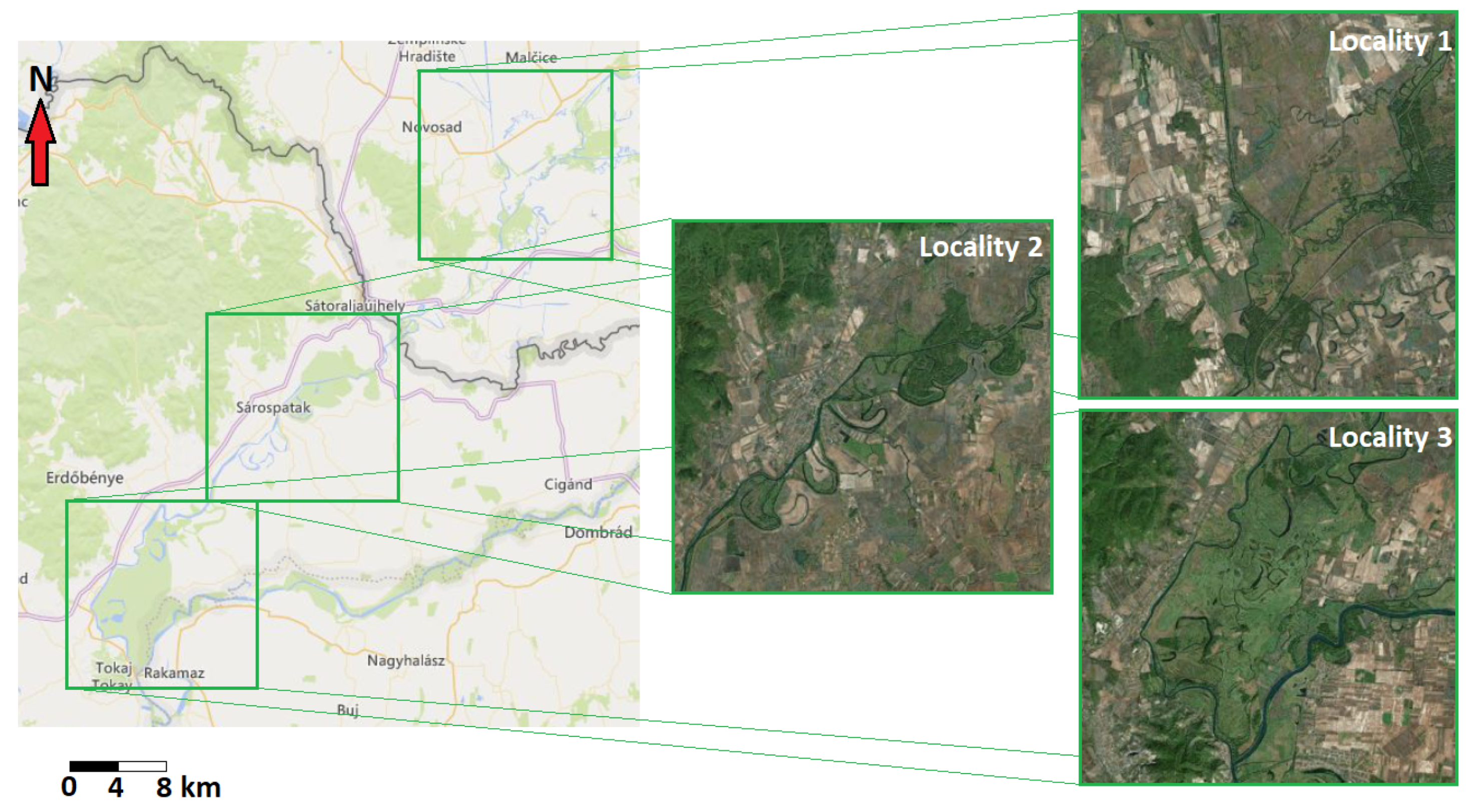
2. Study Area

2.1. Geographical Location

The Bodrog River is one of the rivers located in eastern Slovakia in the East Slovakian lowland. The beginning of the Bodrog River is near the municipalities of Zemplín and Svätá Mária with approximate WGS 84 geographic coordinates of 48.454512° N and 21.819570° E. The Bodrog River begins by the confluence of two rivers, Ondava and Latorica. The river flow continues further southwest towards the Slovakian-Hungarian state border while the river Ošva flows into it. In the Hungarian territory, the rivers Roňava, Kaprona, Suta, Radvány, Tolcsva, and other smaller streams gradually flow into Bodrog. The mouth of the river Bodrog is tributary to the Hungarian river Tisza, in the place near the Hungarian town Tokaj. The length of the Bodrog river is 67 km, 15 km of which flows through the territory of Slovakia, and the remaining 52 km flows through Hungary. The catchment area of the Bodrog is the lowest place in the Slovak Republic, specifically near the municipalities of Klin nad Bodrogom and Borša, in the cadastral territory of Klin nad Bodrogom. Its height is 94.3 m above sea level. Another interesting fact about this river is that it is one of the only navigable rivers in eastern Slovakia. In terms of comparing the length of the stream, Bodrog is the eighth longest river in Slovakia. Moreover, the Bodrog River is also one of the rivers with the maximal possible culmination of the water level in Slovakia. On occasion, the difference can reach up to 7 m (Figure 1).

2.2. Characteristics of the Study Area

With the advent of river system regulation in the 19th century, many rivers were affected. Bodrog was not an exception, as its riverbed was affected above average due to the regional altitude. There was a significant change in the extent of the riverbed and the length of the river. Preserved historical maps from the period of military mapping of Hungary confirm these changes. A typical feature of river regulation is the number of dead branches along the river. Many flat and permanently flooded areas of the Medzibodrožie (i.e., region in the Bodrog river basin) have thus become area+s with more favourable living conditions. According to the available studies [53], after this period of anthropogenic changes in the development of the riverbed, the transverse length of the river channel was, and remains, in equilibrium.

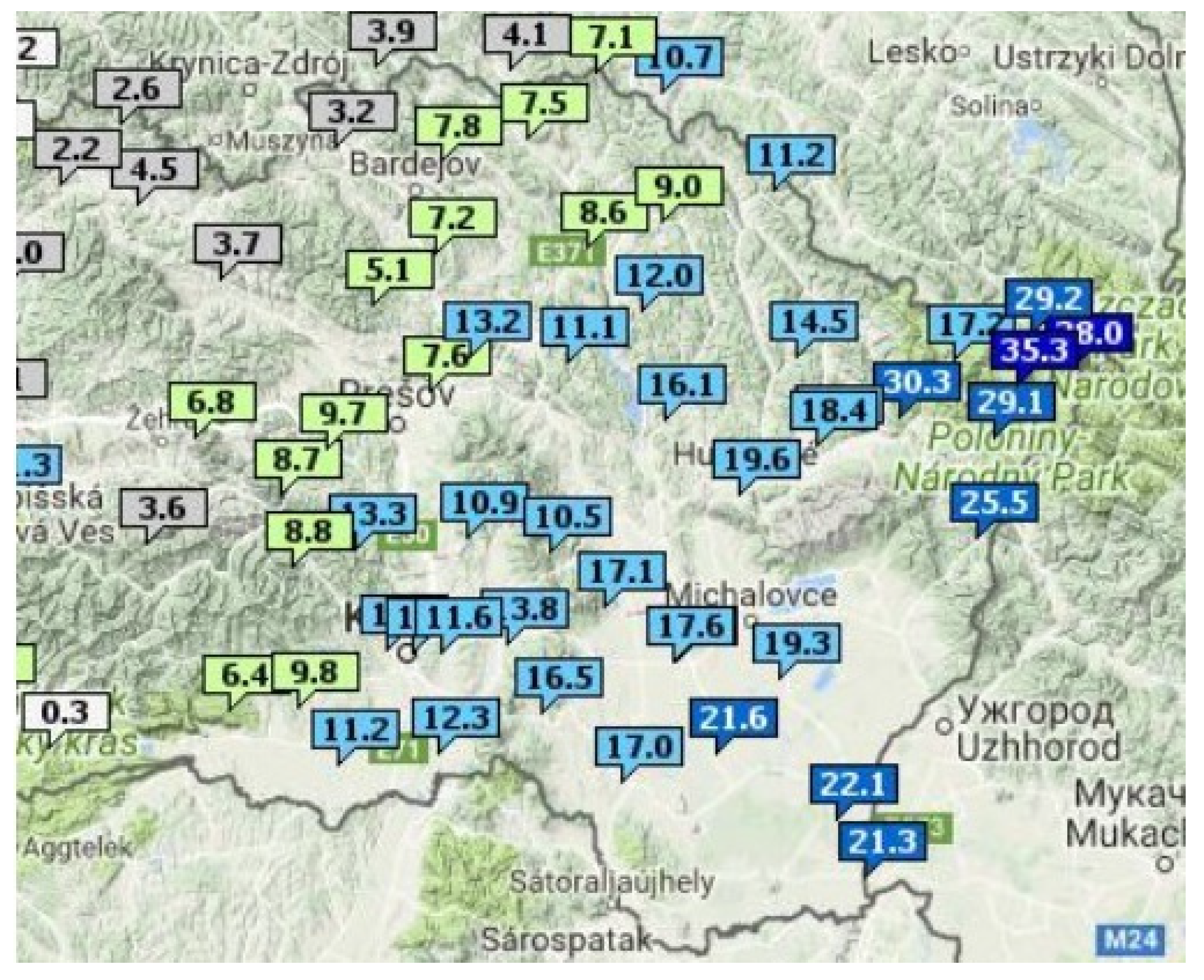
2.3. Climatic and Meteorological Conditions

As for the Bodrog river basin, its characteristic feature is its quite differentiated precipitation throughout the year. Within this locality, the highest annual total rainfall of approximately 1000 mm/year is typical for the Vihorlat Mountains and the surrounding (e.g., mountainous areas near the Slovakian-Ukrainian state border) (Figure 1) [54]. The opposite situation exists a few kilometres south. Specifically, some areas of the East Slovakian lowland belong to areas with the lowest total annual precipitation with an approximate value of 550 mm/year; this includes the areas of Michalovská, Medzibodrožská, and Lastomírska lowlands.

If we take a closer look at the hydrological conditions from December 2017 to February 2018 (Figure 2), this monitored interval was above the annual average. In particular, in this monitored interval, 53 days with flood activity in the Bodrog river basin were recorded [55]. Regarding the flood situation in April 2018, the Slovak Hydrometeorological Institute recorded 17 days in the Bodrog basin with flood activity [56]. Based on these meteorological-hydrological events, a half-yearly interval was chosen for this research, starting in November 2017, representing the natural state of watercourses in the Bodrog basin. This interval thus perfectly captures the behaviour of the water level of the Bodrog River and the adjacent area of its origin due to inundation processes. These inundation processes occurred in December 2017, February 2018, and April 2018 due to high water levels values. The following table provides the exact values of the culmination of the water level for better imagination (

Table 1. The table of culminating water levels and flows in selected flow stations in the temporal interval from November 2017 to March 2018. This table also shows data on the maximum water level and information about the N-year and the declared levels of flood activity [55,56].

Flow Station Name	River Name	Date	Hour	Hmax [cm]	Qmax [m3/s]	N-Year	Flood STAGE 1
Streda nad Bodrogom		19 December 2017	07:15	868	650	2	3 (850 cm)
	Bodrog	7 February 2018	07:15	650	296	<1	1 (650 cm)
		7 April 2018	15:00	759	438	<1	2 (700 cm)
Veľké Kapušany	Latorica	18 December 2017	16:45	784	340	5–10	3 (750 cm)
		7 February 2018	09:00	633	99.9	<1	2 (600 cm)
		20 March 2018	09:30	598	85.8	<1	1 (550 cm)
		6 April 2018	02:45	656	115	<1	2 (600 cm)

¹ Flood Stage is based on H_max values at flow stations.

).

Three sites of interest characteristic in significant flood changes were selected to obtain the most accurate results (Figure 3).

3. Materials and Methods

3.1. Materials

3.1.1. Sentinel-1 SAR Satellite Data

SAR images from Sentinel-1 satellites, which are part of the Copernicus program, conducted by the European Space Agency, were used for this research. The Sentinel-1 mission is a constellation of two polar-orbiting satellites (Sentinel-1A and Sentinel-1B), which operate day and night, sensing with a C-band Synthetic Aperture Radar instrument operating at a central frequency of 5.405 GHz, allowing for the acquisition of imagery regardless of weather and illumination conditions [57]. The ability to penetrate through the clouds determines the suitability of the usage of Sentinel-1 images for monitoring changes in water bodies due to floods.

For a more detailed technical specification of the images used, Ground Range Detected GRD product-level data, which does not contain phase information, were used for this research. These data were acquired using the Interferometric Wide Swath IW scanning mode, which obtains data from a 250-kilometre-wide satellite scanning swath with relative orbit 102 [58]. For each monitored month one SAR image was selected. The previous table (

Table 2. Table of used temporal satellite images SAR Sentinel-1 with their parameters.

Title 1	Satellite Type	Orbit Type	Absolute Orbit
27 November 2017	Sentinel-1B	Descending	8404
19 December 2017	Sentinel-1A	Ascending	19,774
12 January 2018	Sentinel-1A	Ascending	20,124
11 February 2018	Sentinel-1B	Ascending	9578
19 March 2018	Sentinel-1B	Ascending	10,103
12 April 2018	Sentinel-1B	Ascending	10,453

) specifies the parameters of the used images. Sentinel-1 products were acquired through the Data Search Vertex platform of the Alaska Satellite Facility portal available at search.asf.alaska.edu. Another way to obtain data was through the Copernicus Open Access Hub available at scihub.copernicus.eu. All acquired images had a spatial resolution of 10 m × 10 m/pixel and polarisation configuration types of VH and VV.

3.1.2. Sentinel-2 Multispectral Satellite Data

Regarding the optical spectrum of remote sensing, the usage of free available multispectral satellite data with a high spatial resolution is useful [7]. These data include multispectral images from the Sentinel-2 satellite [59,60] which are suitable for water body mapping. These data were chosen for research purposes mainly for better spatial and temporal image resolution than the Landsat-8 satellite data due to the higher number of platforms, i.e., a combination of two satellites versus one satellite. The higher spectral resolution of the resulting multispectral image products is also significant (13 versus 11 spectral bands). The characteristics and description of the spectral bands of the Sentinel-2 satellites are available in the following table (

Table 3. List of spectral bands and their characteristics of Sentinel-2 images.

Band Name	Description	Resolution (Spatial) [m]	Band Width [m]	Central Wavelength [μm]
Band 1	Coastal Aerosol	60	20	0.443
Band 2	Blue	10	65	0.490
Band 3	Green	10	35	0.560
Band 4	Red	10	30	0.665
Band 5	Vegetation Red Edge	20	15	0.705
Band 6	Vegetation Red Edge	20	15	0.740
Band 7	Vegetation Red Edge	20	20	0.783
Band 8	NIR	10	115	0.842
Band 8A	Narrow NIR	20	20	0.865
Band 9	Water Vapor	60	20	0.945
Band 10	SWIR-Cirrus	60	30	1.380
Band 11	SWIR	20	90	1.610
Band 12	SWIR	20	180	2.190

). On the other hand, the resulting images from the Sentinel-2 satellites contain cloud spectral bands. It is necessary to eliminate them in data processing. For this reason, the Google Earth Engine (GEE) cloud platform, and its code editor, available at code.earthengine.google.com (02 April 2021), were chosen to obtain the ideal data products. GEE facilitates a fast analysis platform by using Google’s computing infrastructure [61]. It integrates large amounts of Earth remote sensing data and has the advantage of rapid processing and analysing geospatial data.

The optimal choice of Sentinel-2 images for this research was the COPERNICUS/S2_SR image collection. It consists of product level L-2, processed using the program Sen2cor based on input data level L-1C. Sen2cor allows for the application of terrain correction, a correction of the atmosphere and its effects, and so-called cirrus correction, which is a correction of a thin-film type of cloud. Clouds were filtered using a modified algorithm. Subsequently, the final step was the export of data products modified by an algorithm with defined variables.

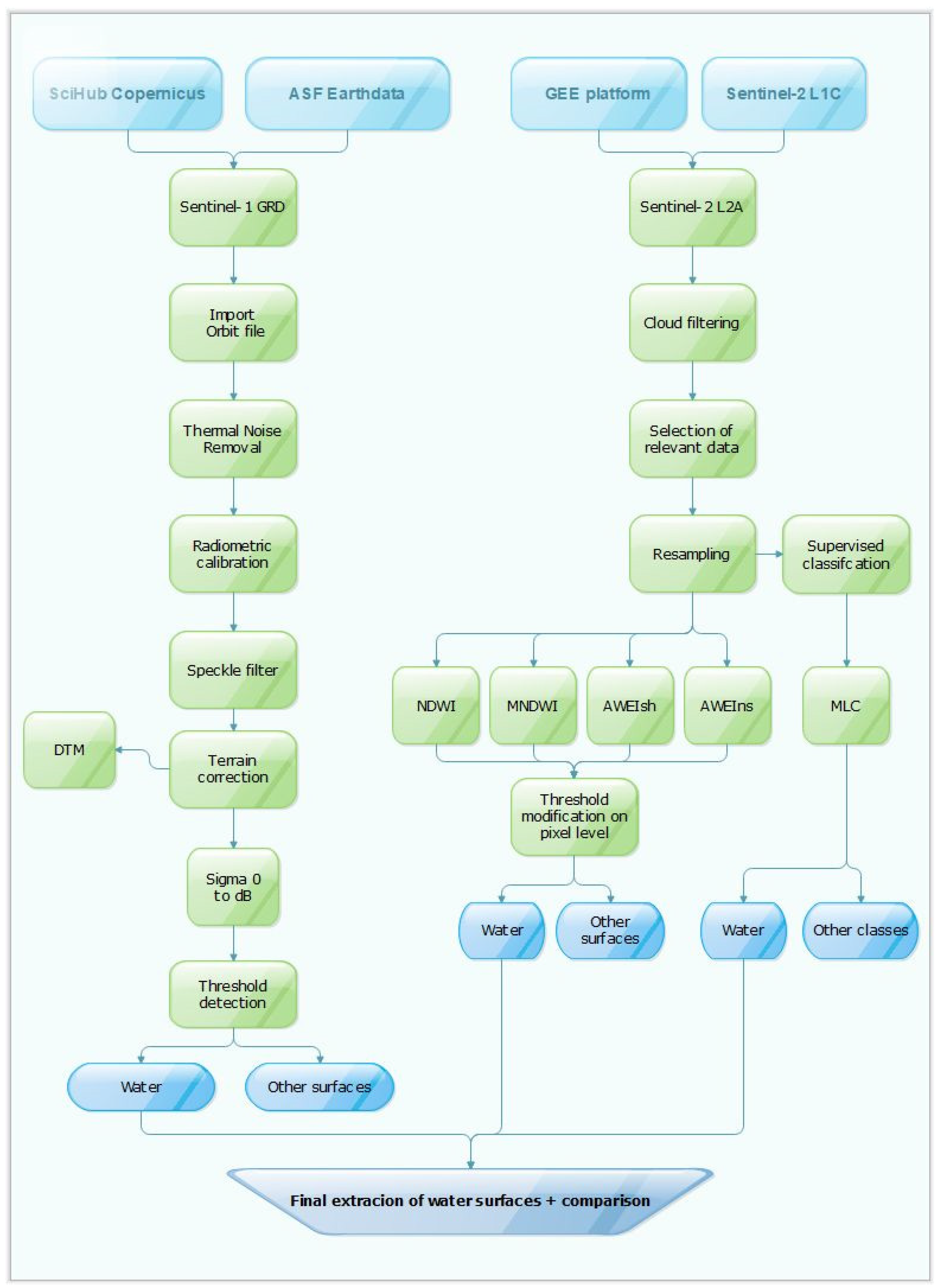
3.2. Methodology

The processing methodology for optical and SAR data is shown in the following workflow diagram (Figure 4).

3.2.1. Water Body Extraction from SAR Data

The process of extracting water surfaces from SAR images consists of several steps. The orbital information is not always included in the data product, as it takes some time to calculate the exact orbital parameters. Therefore, the function “apply orbit file” was used to obtain accurate information about the orbit, i.e., the position and speed of the satellite. At the same time, the orbit file application can improve geocoding and obtain more accurate processing results. In the next phase, it was necessary to eliminate thermal noise from the SAR image, which arises at low energy backscattered SAR signal. Thermal noise is present mainly in cross-polarised channels. Using radiometric calibration, the conversion of SAR image intensity to Sigma 0 values is also an important step [51]. Radar-noise filtering is also relevant in SAR image processing. There are currently several filtering tools available that compare this research. The last step in preprocessing Sentinel-1 GRD products is the Doppler terrain correction application. Its main goal is to eliminate topographic distortions using digital elevation model DEM and transform SAR images into cartographic projection [62].

3.2.2. Water Body Extraction from Optical Data

In relation to the process of obtaining information about water objects and areas on the Earth’s surface, spectral indices based on the mathematical principle are of great importance. There are two methods of obtaining information about water on the Earth’s surface using spectral bands. The first method is the Single-band Method, which consists of selecting a band and setting a threshold value for distinguishing land and water. The second and more effective way is to use the multi-band method. This extraction method includes calculating the ratio between two spectral bands. The first of them represents the region of visible wavelengths of electromagnetic radiation and the second represents near-infrared radiation. Based on this, several spectral indices for water extraction were developed to obtain information about water surfaces.

The first and the most widely used spectral index for the extraction of water surfaces is the Normalized Difference Water Index NDWI [63]. It was developed in 1996 based on the Normalized Difference Vegetation Index NDVI. The main goal of the NDWI index is to maximise the reflectance of water by using green wavelengths, minimising the low reflectance of Near-Infrared Radiation NIR by water features, and taking advantage of the high reflectance of NIR by vegetation and soil features [63]:

$$\mathrm{NDWI}=\frac{GREEN-NIR}{GREEN+NIR}$$

(1)

Another tool for determining water areas is the Modified Normalized Difference-Water Index MNDWI [64]. The development of this type of spectral index of water surfaces occurred in 2006. It uses the visible green light and also the Short-Wave Infrared Radiation SWIR for the calculation due to the more intense absorption of SWIR radiation compared to NIR. It follows that the use of the spectral index MNDWI is justified for water extraction if the multispectral image product contains the SWIR band. A significant advantage of using the MNDWI index is the detection of water bodies in urban areas (64). However, the disadvantage is the weak ability to detect water bodies with high sediment concentrations [40]:

$$\mathrm{MNDWI}=\frac{GREEN-SWIR1}{GREEN+SWIR1}$$

(2)

The need for continuous improvement and refinement of the calculation of the extraction of water surfaces is essential. For this reason, several indices have been developed over the years to try to eliminate misleading information, such as topographic shadows, cloud shadows, built-up areas, snow, and ice [32]. For these purposes, the Automated Water Extraction Index, which consists of two separate indices, was developed in 2014. The first is the AWEI_nsh index formulated to effectively eliminate non-water pixels, including dark built surfaces in areas with an urban background [65]. This index enhances the separation of water pixels from non-water sources [66]:

$${\mathrm{AWEI}}_{\mathrm{nsh}}=4·\left(GREEN-SWIR1\right)-\left(0.25·NIR+2.75·SWIR2\right)$$

(3)

The SWIR2 band represents Short-Wave Infrared Light, but with a higher mean wavelength of 2.190 μm. On the other hand, the AWEI_nsh index assumes insufficient and inefficient elimination of shadow-containing pixels. For this reason, the AWEI_sh index was formulated to improve the accuracy of the extraction of aqueous elements in the following form:

$${\mathrm{AWEI}}_{\mathrm{sh}}=BLUE+2.5·GREEN-1.5·\left(NIR+SWIR1\right)-0.25·SWIR2$$

(4)

On the other hand, high-reflective surfaces may be a part of the wrong classification. Typical objects include ice, snow, or certain types of roofs in urban areas. A significant improvement over the AWEI_nsh index is the implementation of the BLUE band into the calculation.

3.2.3. Accuracy Assessment

The quantitative accuracy assessment process includes comparing the final water masks pixels with a reference background image (freely available high spatial resolution optical imagery Maxar from the Google Earth Pro platform, also visually compared with available aerial orthophotos). With the help of the following four statistical indicators of accuracy: Producer accuracy (PA) [67], User accuracy (UA) [68], Overall accuracy (OA) [69], and Kappa statistical coefficient (Kappa) [70], it is possible to obtain statistical percentage reliability of the results.

$$UA=\frac{TP}{TP+FP}$$

(5)

$$PA=\frac{TP}{TP+FN}$$

(6)

$$OA=\frac{TP+TN}{T}$$

(7)

$$Kappa=\frac{T·\left(TP+TN\right)-\left[\left(TP+FP\right)·\left(TP+FN\right)+\left(FN+TN\right)·\left(FP+TN\right)\right]}{TP+FN}$$

(8)

The True Positives (TP) represents all correctly extracted pixels of water. The False Positives (FP) parameter is the opposite, i.e., the number of pixels of incorrect extraction. The third component of the calculation accuracy is True Negatives (TN), which represents non-water correctly extracted pixels. The False Negatives (FN) describes pixels with incorrect water extraction. Finally, the T component symbolises the number of all pixels.

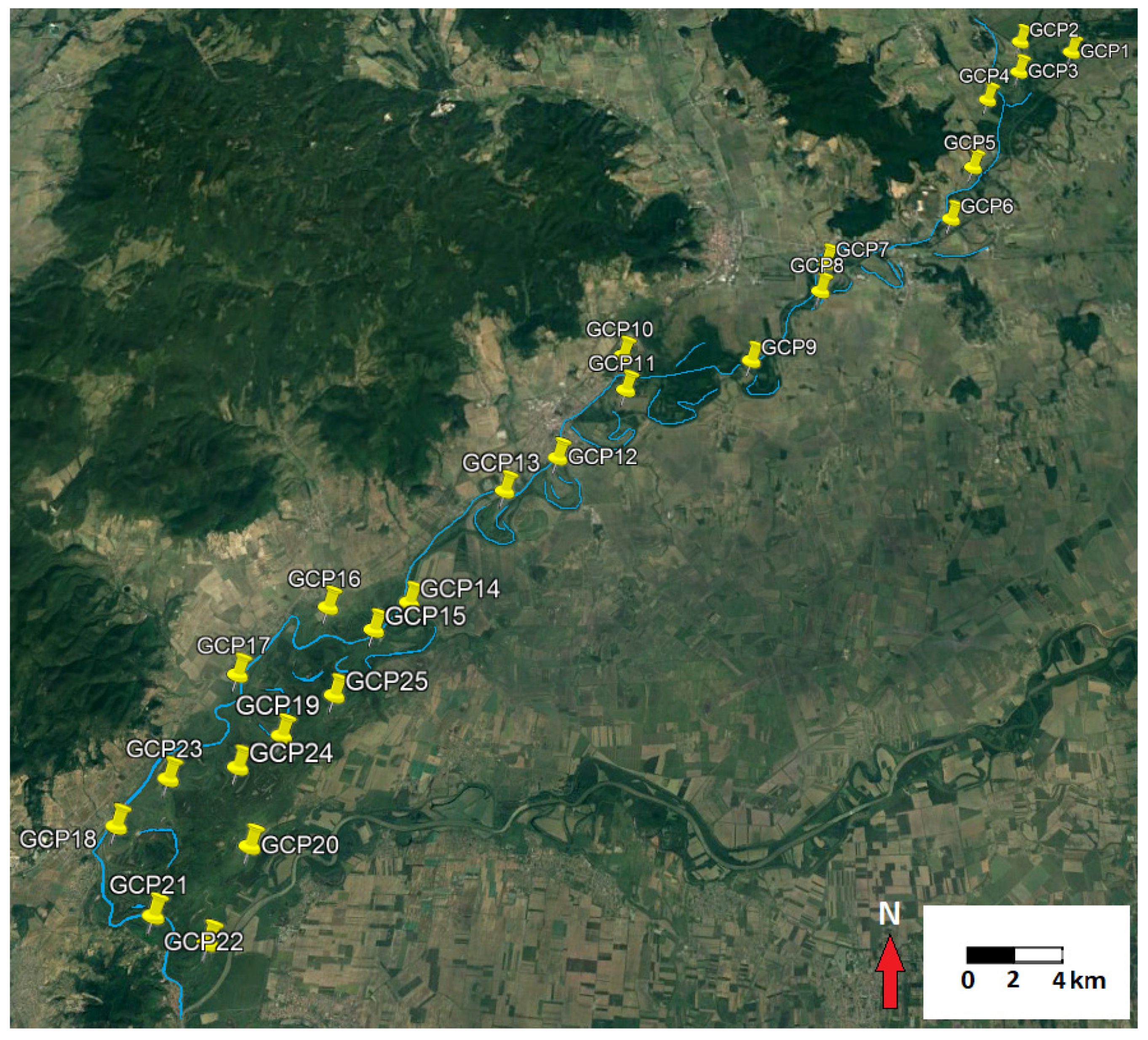
3.2.4. Ground Control Points selection

A significant factor in SAR images is radar signal polarisation. Therefore, the discrimination of inundated areas can be optimised by selecting the most suitable polarisation of the radar waves [71]. Therefore, a comparison of the backscattered signal strength values for both types of Sentinel-1 SAR image polarizations, is necessary to find and choose the correct SAR polarisation type for water extraction through ground-control points (Figure 5).

GCPs have been selected in particular areas close to the Bodrog river bed outside the floodplain processes. Most of these areas were characterized by rough surfaces due to the agricultural activities carried out. They were also characterized by lower vegetation cover, precisely to obtain the optimum value of backscattered SAR signal intensity. All GCPs were chosen in the flooded area, thus the pixel intensity was evaluated before and during the flood event.

4. Results

4.1. SAR Calibration Threshold Results

For comparison, the intensity of pixels was used, converted into a physical quantity, which is called the backscatter coefficient, and expressed in decibels (dB). In obtained values of intensity in dB, it is possible to see minimal differences between VV and VH polarisation during the flood activity. They range from −27 to −23 dB for VH polarisation and from −26 to −20 dB for the type of polarisation referred to as VV. The following image shows the intensity comparison results (Figure 6).

Based on the obtained intensity values, it can be found that the VV polarisation is greatly influenced by the heterogeneity of the environment, but especially by the roughness of the terrain. When observing the extent of inundation under VH polarisation in the selected temporal range (i.e., in winter months), the results are influenced by snow cover. The results are influenced by gently irrigated soil due to melting snow or prolonged rainfall in the spring months. A VH and VV polarisation comparison in 02/2018 (

Table 4. The comparison of accuracy evaluation of water bodies extraction using VV and VH polarisation configuration in 02/2018.

Temporal Interval	Locality	Polarization Type	PA [%]	UA [%]	OA [%]	Kappa
February 2018	L1	VV	77.4	85.7	89.7	0.789
		VH	79.6	78.3	91.1	0.737
	L2	VV	82.4	90.2	95.2	0.874
		VH	84.6	86.8	94.9	0.897
	L3	VV	84.9	93.1	98.6	0.917
		VH	88.3	87.4	97.6	0.899

) shows that areas with higher soil moisture are better identifiable in the VH polarisation configuration. In contrast, open water areas are slightly more pronounced in the VV configuration, as confirmed by another research [72]. Thus, there are fewer incorrectly classified moist soil pixels than water bodies. It validates the results of User Accuracy [73]. As also stated in [74], it is possible to say that VV polarisation has better potential to identify partially submerged features, which can be helpful for flood damage assessment.

Based on previous results, images with VH polarisation show a higher number of areas than water areas compared to VV polarisation than VV polarisation images. The result is an increasing number of false positives [75]. This phenomenon occurs since cross-polarisation images produce a wider range of backscatter values. It leads to a potential overlap with the low backscatter values associated with water [73,76] which causes incorrect classification of water bodies.

Another advantage of selecting images with a VV polarisation configuration is the relative variability in intensity before and after inundation, with the VV polarisation type of Sentinel-1 images (Figure 7). It requires a clear definition of the Sigma 0 intensity threshold. Smooth water bodies also cause the backscatter to fall even further to even lower negative values.

Thus, in conclusion, it is possible to summarise that the VV type is a more suitable polarisation configuration for mapping water surfaces. Finding a more suitable SAR polarisation configuration for water mapping was chosen mainly because the polarisation type specification is not unambiguously defined in the processing procedures and hence, in the scientific literature.

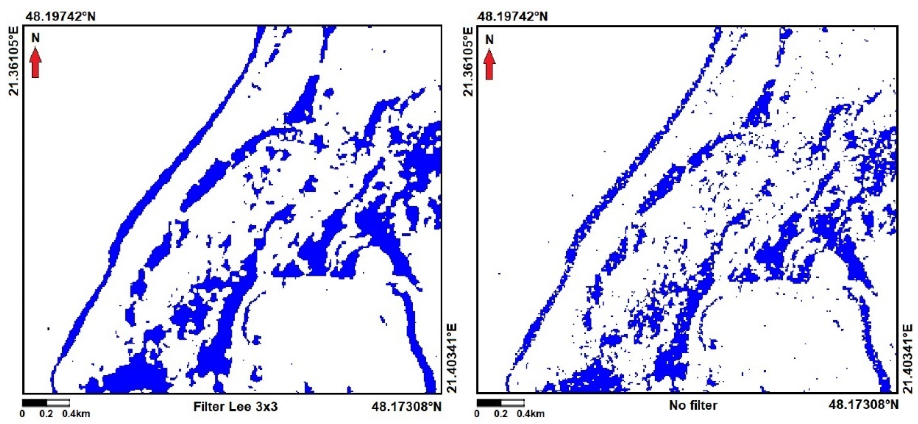
4.2. Radar Noise Elimination Results

As mentioned in the previous chapter, radar-noise filtering plays an important role in SAR-image processing. The results of applying the mentioned filtering tools to remove radar noise show that the images contain several times less random radar noise pixels after applying the filters. By considering the width of the Bodrog channel and the extent of the inundated area, it can be concluded that the use of filters with window sizes 7 × 7, 9 × 9 and larger, appears to be an ineffective way of eliminating radar noise. Comparison of the water masks in the selected area of Locality 3, with and without radar noise filtering (Lee 3 × 3 filter) (No filter), shows that the filtered image contains a minimum of unwanted noise pixels with high backscatter. This ensures continuity in the extraction of water areas and minimisation of random noise outside the water areas (Figure 8).

A water mask comparison was also performed for other radar noise-filtering tools, i.e., for Lee with larger window size, Refined Lee, Gamma Map, and Lee Sigma filter. This comparison revealed that the results contain statistically significant variations that not only depend on the filter used but also on the window size. The unfiltered image contains a lot of dark radar noise pixels, so the resulting range of water areas is both above average and not completely accurate. Thus, it can be said that the application of an arbitrary filter to reduce radar noise prevents errors in quantitative calculations. On the other hand, the use of larger windows (e.g., the Lee filter with a 7 × 7 window size) causes a part of the averaged pixels in the watercourse channel area to be used as a water-free area after the calculation (mainly by changing the spatial resolution of the image). Therefore, its use is suitable for monitoring larger water areas, not narrower river channels. Various types of scientific publications focused on applying the Lee and Lee Sigma filters when investigating this issue. From the numerical and graphical results obtained, the use of the Lee filter appears to be the most advantageous, mainly due to its ability to quite effectively minimise the presence of pixels that are outside the inundated area. The following summary table shows the results in the selected specific area of Site 3 (

Table 5. Results of the extent of water surfaces during the inundation in the selected Locality 3.

Type of Speckle Filter	Window Size	Number of Water Pixels	Extend of Water Bodies [km2]
No Filter	-	17,197	1.720
Lee	3 × 3	14,525	1.453
Lee	5 × 5	15,094	1.509
Lee	7 × 7	10,615	1.062
Lee Sigma	5 × 5	13,889	1.389
Refined Lee	-	15,730	1.573
Gamma MAP	3 × 3	14,645	1.465
Gamma MAP	5 × 5	12,795	1.280

).

The previous table shows that the appropriate window sizes are 3 × 3 or 5 × 5. However, the use of a 5 × 5 window at Locality 1 appeared to be a less appropriate tool, given the decreasing width of the Bodrog river channel and the extent of the water bodies. For this reason, filtering was carried out using the Lee filter with a window size of 3 × 3 for all 3 localities of interest. It is generally known that the channel is almost twice narrower at these sites than at its confluence with the Tisza. This fact is illustrated by the resulting graph (Figure 9) in the form of the water surface extent values during the flood-free situation in November. The individual sites clearly show that the inaccuracy of the determination of the total water surface area increases as the inundated area increases.

The highest values of the extent of water areas are observed in the month of December. This maximum value is associated with the climatic-hydrological changes in December and the declaration of PA level III on several rivers of the Bodrog river basin. The resulting graph of extracted water areas shows the 6-month variability of the changes in water area extent through a Lee filter with a window size of 3 × 3.

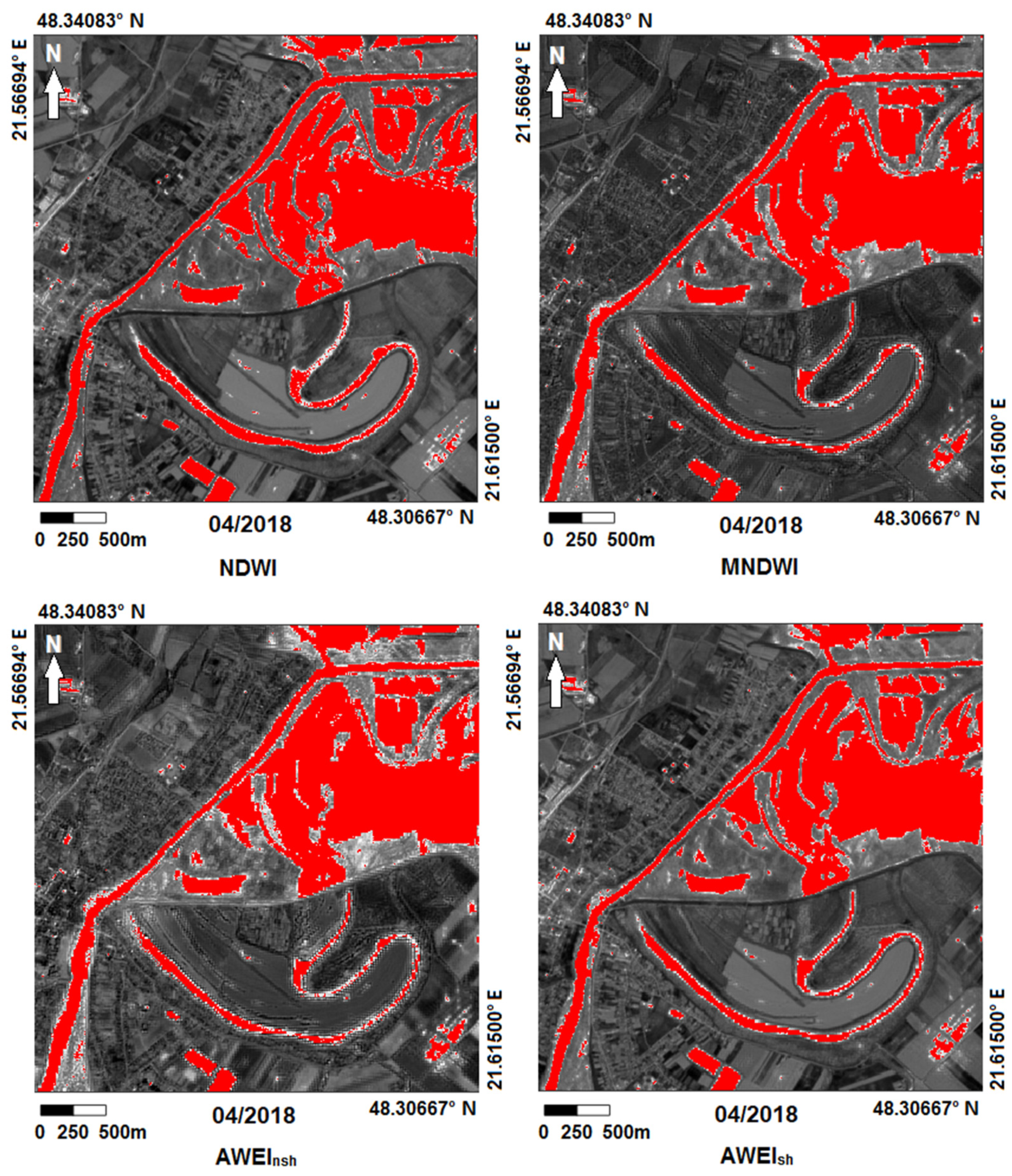
4.3. Results of Comparison of Spectral Indices of Water

For a comparison of the water body extraction using NDWI, MNDWI, AWEI_nsh, and AWEI_sh, it was most appropriate to select the area with all the elements influencing the values of the water pixels. For this reason, an initial comparison was made using the example of the dead arm area of the Keleti Bodrog holtág with the town of Sarospatak and its immediate surroundings. This area is specific in terms of the occurrence of high albedo sites, shady places, and urbanised areas. There is also the possibility of comparing two types of water bodies, i.e., a flowing river and a stagnant water body in a dead channel, partly covered by low vegetation. The comparison of the results in this area yielded the following spectral values (Figure 10).

Based on a visual analysis of the results in this area, it is possible to say that all types of spectral indices increase the separation of water bodies from other non-water elements of the landscape. Of course, each of them has its group of advantages and disadvantages when extracting water.

• NDWI—The water surfaces extraction was continuous. The most significant values of errors were in built-up areas and their shadows with the uncertain distribution. It means that some objects of the urban areas show positive values in the results. Additionally, the increasing presence of additional noise is difficult to eliminate.
• MNDWI—The process of extraction of water bodies was sufficient, with a few exceptions. The disadvantage of using the MNDWI index is its implementation in urban areas with high albedo. The main error factors include the shadows of buildings in built-up areas for the SWIR bands. On the other hand, the separation of urban areas from water surfaces was clear. The slight deterioration in spatial resolution is also visible.
• AWEI_nsh—The extraction with this index was relatively successful. The shadow distribution of the built-up areas was almost identical to that of the MNDWI index. However, in terms of shortcomings, there were significant problems with the shadows of the clouds in February and March. On the images from these months, the cloud filtration process of Sentinel-2 had some cloud coverage limitations.
• AWEI_sh—Areas with a high albedo, like MNDWI, can be considered the significant source of error. It is because soil, vegetation, and built-up classes have smaller negative values, which reflect more SWIR light than green light. On the other hand, the extracted water areas look continuous, without significant changes compared to the previous indices. The graphical representation of the results is as follows (Figure 11).

Regarding the numerical interpretation of the results, the final water masks are different in terms of the extent of the water surfaces. Specifically, in this selected area, water areas in the range from 2.6 to 2.8 km² were achieved (

Table 6. Numerical comparison of water masks pixels and extend of water bodies by four spectral indices in the selected area.

Spectral Index Type	Number of Water Pixels	Extend of Water Bodies [km2]
NDWI	26,212	2621
MNDWI	27,769	2777
AWEInsh	28,239	2824
AWEIsh	26,571	2657

). This range represents an interval with a maximum difference of 0.2 km².

It is clear from this table that the slightly overestimated results for the AWEI_nsh index are likely due to the presence of shadows in the images. On the other hand, water body extraction using the NDWI and AWEI_sh water indices shows that the results are different by only a few tens of square meters from each other. This fact is the same for other monitored images.

4.4. Results of Supervised Classification

Image classification was used to compare the results of water bodies extraction by mathematical spectral indices. Supervised classification based on the Maximum Likelihood Classifier algorithm in the SNAP 8.0 platform is a suitable tool for this comparison. Firstly, creating a New Vector Data Container with polygons is appropriate. Then, polygons of data samples representing selected classification classes, i.e., water and other vegetation soil elements such as forests, bare soil and urban areas, crops, and low vegetation, were assigned to the data samples. In the example of a classified image from Locality 3, the percentage of water areas is 17.022% of pixels from the whole image scene (Figure 12). After conditional calculation, we obtained a numerical range of water bodies, at a value of 30.422 km² after conversion into a binary mask.

Regarding the quantitative classification accuracy assessment (

Table 7. The results of accuracy evaluation of extracted water masks.

Temporal Interval	Locality	Extraction Method	PA [%]	UA [%]	OA [%]	Kappa
November 2017	L2	S2 NDWI	80.4	76.7	86.7	0.689
		S2 MLC Classification	78.6	56.9	84.9	0.497
	L3	S2 NDWI	84.9	72.3	90.6	0.617
		S2 MLC Classification	79.8	68.4	88.2	0.529
January 2018	L2	S2 NDWI	92.6	84.2	95.5	0.756
		S2 MLC Classification	91.7	80.7	93.1	0.689
	L3	S2 NDWI	95.4	90.4	97.4	0.669
		S2 MLC Classification	94.1	88.6	96.0	0.541
February 2018	L2	S2 NDWI	88.2	84.6	91.4	0.903
		S2 MLC Classification	87.0	81.7	90.2	0.816
	L3	S2 NDWI	83.9	75.4	89.7	0.884
		S2 MLC Classification	82.6	76.3	88.6	0.769
March 2018	L2	S2 NDWI	84.7	81.6	89.4	0.739
		S2 MLC Classification	82.9	78.9	88.6	0.697
	L3	S2 NDWI	87.3	79.0	87.2	0.788
		S2 MLC Classification	86.7	77.3	86.3	0.713
April 2018	L2	S2 NDWI	92.1	83.3	94.7	0.887
		S2 MLC Classification	91.7	81.2	93.8	0.864
	L3	S2 NDWI	95.6	91.0	97.8	0.960
		S2 MLC Classification	94.7	86.4	96.9	0.958

), a comparison of MLC supervised classification with water extraction via the NDWI spectral index was performed. From the graphical and numerical results obtained, it can be seen that the implementation of the Maximum Likelihood Classifier supervised classification method yields relatively reliable results. These results are comparable to the method of water-body extraction through water spectral indices.

5. Discussion

Comparison of SAR and Multispectral Results

Of the SAR images acquired for the site of interest, almost all data are usable for water extraction purposes, as they are acquired under any weather conditions and at any acquisition time. Thus, a considerably larger temporal range is available. The data thus provide up-to-date information on changes in a relatively short time frame (exceptionally, even a few hours after a particular change). Of course, the use of SAR data for river and water body-extraction purposes introduces several drawbacks to the processing, including inaccuracies in the mapping of some stream margins and water bodies caused by the presence of vegetation in the shore areas. Additionally, the resulting extracted water surface masks may be affected by the mixing of multiple pixels near riverbanks. Specifically, the usage of VH polarisation configuration shows wider variability of backscattering in vegetation areas due to volume scattering, confirmed in these publications [77,78].

On the other hand, considering the use of Sentinel-2 multispectral imagery, it is clear from the previous chapters that there are numerous ways to obtain information about water bodies in the landscape based on these data. Regarding the inter-comparison between Sentinel-1 and Sentinel-2 data, the advantages of using multispectral images can be characterised as better resolution of the resulting water masks, resulting in a more coherent final appearance of the watercourse mask and its channel, as well as in [79]. Additionally, there is also a demonstrably better ability to detect the signal in riverbank areas (Figure 13).

Of course, the use of Sentinel-2 MSI data for water extraction is also characterised by several drawbacks, including the presence of clouds. Even though cloud filtering was performed in the GEE environment in the preprocessing steps, there was excessive cloud cover in the December 2017 period. This resulted in insufficient cloud filtering, and for this reason, these data products were excluded and were not further compared. Additionally, excessive cloud cover was responsible for excluding Site L1 from the water extraction process and subsequent comparison of results. Increasing noise values due to image processing can be considered as another disadvantage. Therefore, it is necessary to compare several spectral indices and their results for the site of interest, which is the subject of this research. Another disadvantage is the fact that if the image classification method is not used correctly, situations can arise where the signal is reflected from the bottom in areas of shallow, stagnant water, confirmed by this research [80]. This phenomenon thus significantly distorts the resulting values.

Regarding the Sentinel-1 SAR satellite images, the water surfaces show strong backscatter contrast. This characteristic is typical for continental water bodies and river systems without the presence of significant surface waves. However, this type of data needs to be corrected (geometric and radiometric correction), and SAR filtering tools should also be applied. Post-comparisons of the different parameters show that the use of a polarisation configuration of the VV has a more pronounced effect on the backscatter values from the water surfaces with the presence of vegetation due to the double-bounce effect [81,82]. Considering the elimination of the speckle effect, we can say that it partially reduces the resolution quality of the images. For this reason, when testing the filtering tools, Lee filtering, as well as the example in [83], with a window size of 3 × 3, was chosen as the most suitable option with sufficient exclusion of false positives. As in other research [84], the threshold segmentation method, based on Otsu’s algorithm, represents a suitable way of interpreting the results (Figure 14).

6. Conclusions

Considering the Sentinel-2 multispectral imagery, the use of this type of data for water surface extraction and mapping purposes is very advantageous. The principal advantage is that they are not as affected by noise as SAR imagery (radar, thermal, random, etc.). On the other hand, some types of Sentinel-2 imagery were not acquired on the same day and time as Sentinel-1 SAR imagery. In the case of comparing river changes due to peak water levels, such a comparison may not provide accurate and desired results. On the other hand, for the purpose of long-term observation of changes in river channel shape, these data are sufficient. Water extraction using spectral indices is, in principle, a reliable tool for obtaining information about water on the Earth. The higher the diversity of spectral indices for water extraction, the more numerous the results, which yields more relevant results (Figure 13). This fact is partially confirmed by the results of the post-comparison of the NDWI, MNDWI and AWEI indices. However, we see slight differences in the resulting values of the range of water areas when using the supervised classification.

When extracting water surface information from Sentinel-2 imagery, it can be said that the threshold segmentation method should be supplemented with the elimination of additional noise for water-extraction purposes. Furthermore, it is appropriate to complement the satellite remote sensing with multispectral data from aerial technology to verify the results. The main advantage of using these data is the considerably higher spatial resolution and the choice of lower flight altitudes during cloudy days. For SAR data, the use of satellite data from so-called Third-Party Missions with a higher spatial resolution (e.g., SAR constellation of 4 COSMO-SkyMed satellites, etc.) can be an advantage. However, the most important improvements in the validity of SAR data results are changes in the evaluation process, such as automation of threshold segmentation (for SAR) or more user-oriented algorithmic processing (e.g., also using the GEE platform).

This paper compared the extraction of water surfaces using SAR and multispectral data. For these purposes, a quartet of spectral indices was used, supplemented by a comparison of SAR cross-polarized and co-polarised channels. The results were also complemented by the MLC classification method. The results were obtained based on the number of water surface extraction methods compared using several methodological approaches and applying these procedures to the online environment, particularly using the Google Earth Engine platform. It presents an efficient algorithmic way of extracting and preprocessing satellite data. For further research, the authors intend to focus more on individual extraction methods with a focus on deep learning or machine learning in the field of water surface extraction.

Studies in the same research area are mainly oriented towards research on water extraction mainly from areas outside Central Europe. Alternatively, they focus on the application of extraction methods to rivers with wider channels and higher flow rates. The application of the use of satellite data with a spatial resolution of 10 m/pixel under specific conditions (homogeneity of the environment, narrower type of river channel, difference between waterlogged and flooded land) has in most cases confirmed the positives or negatives of the individual methodological approaches. At the same time, when using SAR polarisation configurations, the results obtained show the use of co-polarised channels as more advantageous, while a number of researchers prefer the use of cross-polarised channels. Thus, there is no clearly established methodology regarding the polarisation configuration.

Such rapid tracking of regional-scale changes in streamflows has important implications for flood mitigation and socio-economic aspects of individual regions.

References

- Feng, M.; Sexton, J.O.; Channan, S.; Townshend, J.R. A global, high-resolution (30-m) inland water body dataset for 2000: First results of a topographic-spectral classification algorithm. Int. J. Digit. Earth 2016, 9, 113–133. [Google Scholar] [CrossRef] [Green Version]
- Sekertekin, A. A Survey on Global Thresholding Methods for Mapping Open Water Body Using Sentinel-2 Satellite Imagery and Normalized Difference Water Index. Arch. Comput. Method Eng. 2019, 13, 1335–1347. [Google Scholar] [CrossRef]
- Jiang, W.; He, G.; Pang, Z.; Guo, H.; Long, T.; Ni, Y. Surface water map of China for 2015 (SWMC-2015) derived from Landsat 8 satellite imagery. Remote Sens. Lett. 2020, 11, 265–273. [Google Scholar] [CrossRef]
- Yue, H.; Li, Y.; Qian, J.X.; Liu, Y. A new accuracy evaluation method for water body extraction. Int. J. Remote Sens. 2020, 41, 7311–7342. [Google Scholar] [CrossRef]
- Jiang, W.; He, G.; Long, T.; Ni, Y.; Liu, H.; Peng, Y.; Lv, K.; Wang, G. Multilayer Perceptron Neural Network for Surface Water Extraction in Landsat 8 OLI Satellite Images. Remote Sens. 2018, 10, 755. [Google Scholar] [CrossRef] [Green Version]
- Holgerson, M.A.; Raymond, P.A. Large contribution to inland water CO2 and CH4 emissions from very small ponds. Nat. Geosci. 2016, 9, 222–226. [Google Scholar] [CrossRef]
- Pekel, J.F.; Cottam, A.; Gorelick, N.; Belward, A.S. High-resolution mapping of global surface water and its long-term changes. Nature 2016, 540, 418–422. [Google Scholar] [CrossRef]
- Zeleňáková, M.; Fijko, R.; Labant, S.; Weiss, E.; Markovič, G.; Weiss, R. Flood risk modelling of the Slatvinec stream in Kružlov village, Slovakia. J. Clean. Prod. 2019, 212, 109–118. [Google Scholar] [CrossRef]
- Gardner, R.; Barchiesi, S.; Beltrame, C.; Finlayson, C.; Galewski, T.; Harrison, I.; Paganini, M.; Perennou, C.; Pritchard, D.; Rosenqvist, A.; et al. State of the World’s Wetlands and Their Services to People: A Compilation of Recent Analyses. SSRN Electron. J. 2015, 21, 1–21. [Google Scholar] [CrossRef] [Green Version]
- Gergeľová, M.; Kuzevičová, Ž.; Kuzevič, Š.; Sabolová, J. Hydrodynamic modeling and GIS tools applied in urban areas. Acta Montan. Slovaca 2013, 18, 226–233. [Google Scholar]
- Papa, F.; Prigent, C.; Rossow, W.B. Monitoring Flood and Discharge Variations in the Large Siberian Rivers from a Multi-Satellite Technique. Surv. Geophys. 2008, 29, 297–317. [Google Scholar] [CrossRef]
- Michalowska, K.; Glowienka, E.; Hejmanowska, B. Temporal Satellite Images in The Process of Automatic Efficient Detection of Changes of the Baltic Sea Coastal Zone. IOP Conf. Ser. Earth Environ. Sci. 2016, 44, 042019. [Google Scholar] [CrossRef] [Green Version]
- Rahman, M.R.; Thakurb, P.K. Detecting, mapping and analysing of flood water propagation using synthetic aperture radar (SAR) satellite data and GIS: A case study from the Kendrapara District of Orissa State of India. Egypt. J. Remote Sens. Space Sci. 2018, 21, 37–41. [Google Scholar] [CrossRef]
- Tran, H.; Nguyen, P.; Ombadi, M.; Hsu, K.; Sorooshian, S.; Andreadis, K. Improving Hydrologic Modeling Using Cloud-Free MODIS Flood Maps. J. Hydrometeorol. 2019, 20, 2203–2214. [Google Scholar] [CrossRef] [Green Version]
- Szombara, S.; Lewińska, P.; Żądło, A.; Róg, M.; Maciuk, K. Analyses of the Prądnik riverbed Shape Based on Archival and Contemporary Data Sets—Old Maps, LiDAR, DTMs, Orthophotomaps and Cross-Sectional Profile Measurements. Remote Sens. 2020, 12, 2208. [Google Scholar] [CrossRef]
- Tran, H.; Nguyen, P.; Ombadi, M.; Hsu, K.; Sorooshian, S.; Qing, X. A cloud-free MODIS snow cover dataset for the contiguous United States from 2000 to 2017. Sci. Data 2019, 6, 180300. [Google Scholar] [CrossRef]
- Urban, R.; Štroner, M.; Blistan, P.; Kovanič, Ľ.; Patera, M.; Jacko, S.; Ďuriška, I.; Kelemen, M.; Szabo, S. The Suitability of UAS for Mass Movement Monitoring Caused by Torrential Rainfall—A Study on the Talus Cones in the Alpine Terrain in High Tatras, Slovakia. ISPRS Int. J. Geo-Inf. 2019, 8, 317. [Google Scholar] [CrossRef] [Green Version]
- Blistan, P.; Kovanič, L.; Patera, M.; Hurčík, T. Evaluation quality parameters of DEM generated with low-cost UAV photogrammetry and Structure-from-Motion (SfM) approach for topographic surveying of small areas. Acta Montan. Slovaca 2019, 24, 198–212. [Google Scholar]
- Urban, R.; Štroner, M.; Kuric, I. The use of onboard UAV GNSS navigation data for area and volume calculation. Acta Montan. Slovaca 2020, 25, 361–374. [Google Scholar]
- Bazzi, H.; Baghdadi, N.; Ienco, D.; El Hajj, M.; Zribi, M.; Belhouchette, H.; Escorihuela, M.J.; Demarez, V. Mapping Irrigated Areas Using Sentinel-1 Time Series in Catalonia, Spain. Remote Sens. 2019, 11, 1836. [Google Scholar] [CrossRef] [Green Version]
- Lee, J.S.; Pottier, E. Polarimetric Radar Imaging, 1st ed.; CRC Press, Taylor & Francis Group: Boca Raton, FL, USA, 2017; p. 398. [Google Scholar] [CrossRef]
- Dabiri, Z.; Hölbling, D.; Abad, L.; Helgason, J.K.; Sæmundsson, Þ.; Tiede, D. Assessment of Landslide-Induced Geomorphological Changes in Hítardalur Valley, Iceland, Using Sentinel-1 and Sentinel-2 Data. Appl. Sci. 2020, 10, 5848. [Google Scholar] [CrossRef]
- Paluba, D.; Laštovička, J.; Mouratidis, A.; Štych, P. Land Cover-Specific Local Incidence Angle Correction: A Method for Time-Series Analysis of Forest Ecosystems. Remote Sens. 2021, 13, 1743. [Google Scholar] [CrossRef]
- Marzi, D.; Gamba, P. Inland Water Body Mapping Using Multitemporal Sentinel-1 SAR Data. IEEE J. Sel. Top. Appl. Earth Obs. Remote Sens. 2021, 14, 11789–11799. [Google Scholar] [CrossRef]
- Chapman, B.; McDonald, K.; Shimada, M.; Rosenqvist, A.; Schroeder, R.; Hess, L. Mapping Regional Inundation with Spaceborne L-Band SAR. Remote Sens. 2015, 7, 5440–5470. [Google Scholar] [CrossRef] [Green Version]
- Voormansik, K.; Praks, J.; Antropov, O.; Jagomägi, J.; Zalite, K. Flood Mapping with TerraSAR-X in Forested Regions in Estonia. IEEE J. Sel. Top. Appl. Earth Obs. Remote Sens. 2014, 7, 562–577. [Google Scholar] [CrossRef]
- Pulvirenti, L.; Pierdicca, N.; Chini, M.; Guerriero, L. Monitoring Flood Evolution in Vegetated Areas Using COSMO-SkyMed Data: The Tuscany 2009 Case Study. IEEE J. Sel. Top. Appl. Earth Obs. Remote Sens. 2013, 6, 1807–1816. [Google Scholar] [CrossRef]
- Schlaffer, S.; Chini, M.; Dettmering, D.; Wagner, W. Mapping Wetlands in Zambia Using Seasonal Backscatter Signatures Derived from ENVISAT ASAR Time Series. Remote Sens. 2016, 8, 402. [Google Scholar] [CrossRef] [Green Version]
- Brisco, B.; Schmitt, A.; Murnaghan, K.; Kaya, S.; Roth, A. SAR Polarimetric Change Detection for Flooded Vegetation. Int. J. Digit. Earth 2013, 6, 103–114. [Google Scholar] [CrossRef]
- Evans, T.L.; Costa, M.; Tomas, W.M.; Camilo, A.R. Large-scale habitat mapping of the Brazilian Pantanal wetland: A synthetic aperture radar approach. Remote Sens. Environ. 2014, 155, 89–108. [Google Scholar] [CrossRef]
- Hess, L.L.; Melack, J.M.; Affonso, A.G.; Barbosa, C.; Gastil-Buhl, M.; Novo, E.M.L.M. Wetlands of the Lowland Amazon Basin: Extent, Vegetative Cover, and Dual-season Inundated Area as Mapped with JERS-1 Synthetic Aperture Radar. Wetlands 2015, 35, 745–756. [Google Scholar] [CrossRef]
- Kaplan, G.; Avdan, U. Object-based water body extraction model using Sentinel-2 satellite imagery. Eur. J. Remote Sens. 2017, 50, 137–143. [Google Scholar] [CrossRef] [Green Version]
- Work, E.A.; Gilmer, D.S. Utilisation of satellite data for inventorying prairie ponds and lakes. Photogramm. Eng. Remote Sens. 1976, 42, 685–694. [Google Scholar]
- Sivanpillai, R.; Miller, S.N. Improvements in mapping water bodies using ASTER data. Ecol. Inform. 2010, 5, 73–78. [Google Scholar] [CrossRef]
- Huang, C.; Chen, Y.; Wu, J.P. Mapping spatio-temporal flood inundation dynamics at large river basin scale using time-series flow data and MODIS imagery. Int. J. Appl. Earth Obs. Geoinf. 2014, 26, 350–362. [Google Scholar] [CrossRef]
- Li, W.; Du, Z.; Ling, F.; Zhou, D.; Wang, H.; Gui, Y.; Sun, B.; Zhang, X. A Comparison of Land Surface Water Mapping Using the Normalised Difference Water Index from TM, ETM+ and ALI. Remote Sens. 2013, 5, 5530–5549. [Google Scholar] [CrossRef] [Green Version]
- Xie, H.; Luo, X.; Xu, X.; Tong, X.; Jin, Y.; Pan, H.; Zhou, B. New hyperspectral difference water index for the extraction of urban water bodies by the use of airborne hyperspectral images. J. Appl. Remote Sens. 2014, 8, 085098. [Google Scholar] [CrossRef] [Green Version]
- Jiang, H.; Feng, M.; Zhu, Y.; Lu, N.; Huang, J.; Xiao, T. An Automated Method for Extracting Rivers and Lakes from Landsat Imagery. Remote Sens. 2014, 6, 5067–5089. [Google Scholar] [CrossRef] [Green Version]
- Ryu, J.; Won, J.; Min, K. Waterline extraction from Landsat TM data in a tidal flatA case study in Gomso Bay, Korea. Remote Sens. Environ. 2002, 83, 442–456. [Google Scholar] [CrossRef]
- Sun, F.; Sun, W.; Chen, J.; Gong, P. Comparison and improvement of methods for identifying waterbodies in remotely sensed imagery. Int. J. Remote Sens. 2012, 33, 6854–6875. [Google Scholar] [CrossRef]
- Yang, X.; Qin, Q.; Grussenmeyer, P.; Koehl, M. Urban surface water body detection with suppressed built-up noise based on water indices from Sentinel-2 MSI imagery. Remote Sens. Environ. 2018, 219, 259–270. [Google Scholar] [CrossRef]
- Yao, F.; Wang, C.; Dong, D.; Luo, J.; Shen, Z.; Yang, K. High-Resolution Mapping of Urban Surface Water Using ZY-3 Multi-Spectral Imagery. Remote Sens. 2015, 7, 12336–12355. [Google Scholar] [CrossRef] [Green Version]
- Li, X.; He, X.; Yang, G.; Liu, H.; Long, A.; Chen, F.; Liu, B.; Gu, X. Land use/cover and landscape pattern changes in Manas River Basin based on remote sensing. Int. J. Agric. Biol. Eng. 2020, 13, 141–152. [Google Scholar] [CrossRef]
- Liu, H.; He, G.; Peng, Y.; Wang, G.; Yin, R. Dynamic monitoring of surface water in the Tibetan Plateau from 1980s to 2019 based on satellite remote sensing images. J. Mt. Sci. 2021, 18, 2833–2841. [Google Scholar] [CrossRef]
- Sahoo, P.K.; Soltani, S.; Wong, A.K.C. A survey of thresholding techniques. Comp. Vis. Graph. Image Process. 1988, 41, 233–260. [Google Scholar] [CrossRef]
- Rosenfeld, A.; De La Torre, P. Histogram concavity analysis as an aid in threshold selection. IEEE Trans. Syst. Man Cybern. 1983, SMC-13, 231–235. [Google Scholar] [CrossRef]
- Otsu, N. A Threshold Selection Method from Gray-Level Histograms. IEEE Trans. Syst. Man Cybern. 1979, 9, 62–66. [Google Scholar] [CrossRef] [Green Version]
- Kittler, J.; Illingworth, J. On threshold selection using clustering criteria. IEEE Trans. Syst. Man Cybern. 1985, SMC-15, 652–655. [Google Scholar] [CrossRef]
- Tsai, W.H. Moment-preserving thresholding: A new approach. Comp. Vis. Graph. Image Proces. 1985, 29, 377–393. [Google Scholar] [CrossRef]
- Jiang, W.; Ni, Y.; Pang, Z.; Li, X.; Ju, H.; He, G.; Lv, J.; Yang, K.; Fu, J.; Qin, X. An Effective Water Body Extraction Method with New Water Index for Sentinel-2 Imagery. Water 2021, 13, 1647. [Google Scholar] [CrossRef]
- Chen, F.; Chen, X.; Van de Voorde, T.; Roberts, D.; Jiang, H.; Xu, W. Open water detection in urban environments using high spatial resolution remote sensing imagery. Remote Sens. Environ. 2020, 242, 111706. [Google Scholar] [CrossRef]
- Bijeesh, T.; Narasimhamurthy, K. Surface water detection and delineation using remote sensing images: A review of methods and algorithms. Sustain. Water Resour. Manag. 2020, 6, 68. [Google Scholar] [CrossRef]
- Mecser, N.; Demeter, G.; Szabó, G. Morphometric changes of the Bodrog River from the Late 18th century to 2006. AGD Landsc. Environ. 2009, 3, 28–40. [Google Scholar]
- Zeleňáková, M.; Purcz, P.; Poórová, Z.; Alkhalaf, I.; Hlavatá, H.; Portela, M. Monthly Trends of Precipitation in Gauging Stations in Slovakia. Procedia Eng. 2016, 162, 106–111. [Google Scholar] [CrossRef]
- Ministry of Environment of the Slovak Republic. Povodňová Situácia v Zime 2017/2018 na Východnom Slovensku; Slovak Hydrometeorological Institute: Košice, Slovakia, 2018; p. 32. [Google Scholar]
- Ministry of Environment of the Slovak Republic. Povodňová Situácia na Východnom Slovensku v Apríli 2018; Slovak Hydrometeorological Institute: Košice, Slovakia, 2018; p. 29. [Google Scholar]
- Filipponi, F. Sentinel-1 GRD Preprocessing Workflow. Proceedings 2019, 18, 11. [Google Scholar] [CrossRef] [Green Version]
- User Guides—Sentinel-1 SAR—Acquisition Modes—Sentinel Online. Available online: https://sentinel.esa.int/web/sentinel/user-guides/sentinel-1-sar/acquisition-modes (accessed on 30 August 2021).
- Du, Y.; Zhang, Y.; Ling, F.; Wang, Q.; Li, W.; Li, X. Water Bodies’ Mapping from Sentinel-2 Imagery with Modified Normalized Difference Water Index at 10-m Spatial Resolution Produced by Sharpening the SWIR Band. Remote Sens. 2016, 8, 354. [Google Scholar] [CrossRef] [Green Version]
- Yang, X.; Zhao, S.; Qin, X.; Zhao, N.; Liang, L. Mapping of Urban Surface Water Bodies from Sentinel-2 MSI Imagery at 10 m Resolution via NDWI-Based Image Sharpening. Remote Sens. 2017, 9, 596. [Google Scholar] [CrossRef] [Green Version]
- Zurqani, H.A.; Post, C.J.; Mikhailova, E.A.; Schlautman, M.A.; Sharp, J.L. Geospatial analysis of land use change in the Savannah River Basin using Google Earth Engine. Int. J. Appl. Earth Obs. Geoinf. 2018, 69, 175–185. [Google Scholar] [CrossRef]
- Bayanudin, A.A.; Jatmiko, R.H. Orthorectification of Sentinel-1 SAR (Synthetic Aperture Radar) Data in Some Parts of South-eastern Sulawesi Using Sentinel-1 Toolbox. IOP Conf. Ser. Earth Environ. Sci. 2016, 47, 012007. [Google Scholar] [CrossRef]
- McFeeters, S.K. The Use of the Normalized Difference Water Index (NDWI) in the Delineation of Open Water Features. Int. J. Remote Sens. 1996, 17, 1425–1432. [Google Scholar] [CrossRef]
- Xu, H. Modification of normalised difference water index (NDWI) to enhance open water features in remotely sensed imagery. Int. J. Remote Sens. 2006, 27, 3025–3033. [Google Scholar] [CrossRef]
- Feyisa, G.L.; Meilby, H.; Fensholt, R.; Proud, S.R. Automated Water Extraction Index: A new technique for surface water mapping using Landsat imagery. Remote Sens. Enivon. 2014, 140, 23–35. [Google Scholar] [CrossRef]
- Nguyen, U.N.T.; Pham, L.T.H.; Dang, T.D. An automatic water detection approach using Landsat 8 OLI and Google Earth Engine cloud computing to map lakes and reservoirs in New Zealand. Environ. Monit. Assess. 2019, 191, 235. [Google Scholar] [CrossRef]
- Stehman, S.V.; Foody, G.M. Accuracy assessment. In The SAGE Handbook of Remote Sensing; Sage: London, UK, 2009; pp. 297–309. [Google Scholar]
- Story, M.; Congalton, R.G. Accuracy assessment: A user’s perspective. Photogramm. Eng. Remote Sens. 1986, 52, 397–399. [Google Scholar]
- Alberg, A.; Park, J.; Hager, B.; Brock, M.; Diener-West, M. The use of “overall accuracy” to evaluate the validity of screening or diagnostic tests. J. Gen. Intern. Med. 2004, 19, 460–465. [Google Scholar] [CrossRef] [Green Version]
- Stehman, S. Estimating the kappa coefficient and its variance under stratified random sampling. Photogramm. Eng. Remote Sens. 1996, 62, 401–407. [Google Scholar]
- Klemas, V. Remote sensing of floods and flood-prone areas: An overview. J. Coast. Res. 2015, 31, 1005–1013. [Google Scholar] [CrossRef]
- Rao, P.; Rao, K.; Kubo, S. Proceedings of International Conference on Remote Sensing for Disaster Management; Springer: Cham, Switzerland, 2019. [Google Scholar]
- Clement, M.; Kilsby, C.; Moore, P. Multi-temporal synthetic aperture radar flood mapping using change detection. J. Flood Risk Manag. 2017, 11, 152–168. [Google Scholar] [CrossRef]
- Manjusree, P.; Prasanna Kumar, L.; Bhatt, C.; Rao, G.; Bhanumurthy, V. Optimization of threshold ranges for rapid flood inundation mapping by evaluating backscatter profiles of high incidence angle SAR images. Int. J. Disaster Risk Sci. 2012, 3, 113–122. [Google Scholar] [CrossRef] [Green Version]
- Cao, H.; Zhang, H.; Wang, C.; Zhang, B. Operational Flood Detection Using Sentinel-1 SAR Data over Large Areas. Water 2019, 11, 786. [Google Scholar] [CrossRef] [Green Version]
- Twele, A.; Cao, W.; Plank, S.; Martinis, S. Sentinel-1-based flood mapping: A fully automated processing chain. Int. J. Remote Sens. 2016, 37, 2990–3004. [Google Scholar] [CrossRef]
- Dutta, U.; Singh, Y.K.; Prabhu, T.S.M.; Yendargaye, G.; Kale, R.G.; Kumar, B.; Khare, M.; Yadav, R.; Khattar, R.; Samal, S.K. Flood Forecasting in Large River Basins Using FOSS Tool and HPC. Water 2021, 13, 3484. [Google Scholar] [CrossRef]
- Rubel, O.; Lukin, V.; Rubel, A.; Egiazarian, K. Selection of Lee Filter Window Size Based on Despeckling Efficiency Prediction for Sentinel SAR Images. Remote Sens. 2021, 13, 1887. [Google Scholar] [CrossRef]
- Zhang, M.; Chen, F.; Liang, D.; Tian, B.; Yang, A. Use of Sentinel-1 GRD SAR Images to Delineate Flood Extent in Pakistan. Sustainability 2020, 12, 5784. [Google Scholar] [CrossRef]
- Tsyganskaya, V.; Martinis, S.; Marzahn, P. Flood Monitoring in Vegetated Areas Using Multitemporal Sentinel-1 Data: Impact of Time Series Features. Water 2019, 11, 1938. [Google Scholar] [CrossRef] [Green Version]
- Touzi, R.; Deschamps, A.; Rother, G. Phase of Target Scattering for Wetland Characterization Using Polarimetric C-Band SAR. IEEE Trans. Geosci. Remote Sens. 2009, 47, 3241–3261. [Google Scholar] [CrossRef]
- Tsyganskaya, V.; Martinis, S.; Marzahn, P.; Ludwig, R. Detection of Temporary Flooded Vegetation Using Sentinel-1 Time Series Data. Remote Sens. 2018, 10, 1286. [Google Scholar] [CrossRef] [Green Version]
- Notti, D.; Giordan, D.; Caló, F.; Pepe, A.; Zucca, F.; Galve, J.P. Potential and Limitations of Open Satellite Data for Flood Mapping. Remote Sens. 2018, 10, 1673. [Google Scholar] [CrossRef] [Green Version]
- Bolanos, S.; Stiff, D.; Brisco, B.; Pietroniro, A. Operational Surface Water Detection and Monitoring Using Radarsat 2. Remote Sens. 2016, 8, 285. [Google Scholar] [CrossRef] [Green Version]