Estimating the Evaporative Cooling Effect of Irrigation within and above Soybean Canopy

Abstract

Vegetation with an adequate supply of water might contribute to cooling the land surface around it through the latent heat flux of transpiration. This study investigates the potential estimation of evaporative cooling at plot scale, using soybean as example. Some of the plants’ physiological parameters were monitored and sampled at weekly intervals. A physics-based model was then applied to estimate the irrigation-induced cooling effect within and above the canopy during the middle and late season of the soybean growth period. We then examined the results of the temperature changes at a temporal resolution of ten minutes between every two irrigation rounds. During the middle and late season of growth, the cooling effects caused by evapotranspiration within and above the canopy were, on average, 4.4 K and 2.9 K, respectively. We used quality indicators such as R-squared (R²) and mean absolute error (MAE) to evaluate the performance of the model simulation. The performance of the model in this study was better above the canopy (R² = 0.98, MAE = 0.3 K) than below (R² = 0.87, MAE = 0.9 K) due to the predefined thermodynamic condition used to estimate evaporative cooling. Moreover, the study revealed that canopy cooling contributes to mitigating heat stress conditions during the middle and late seasons of crop growth.

1. Introduction

Global warming is raising the frequency and intensity of extreme weather events [1]. Regional temperatures are expected to increase more, and with greater variability, than the mean global temperature [2], resulting in more intense and longer heatwaves [3]. Heatwaves have exerted a great deal of additional stress on ecosystems over the past decade [4]. These extreme heat events can produce significant physiological consequences for ecological systems [5,6] triggering mortality, abrupt demographic disruptions, and ecosystem reconfigurations [7,8,9]. Heatwaves have a great effect not only on biodiversity, but also on human health—increasing human discomfort, as well as reducing labour productivity [10], which causes humans to seek cool spots for leisure under extreme heat. Heatwaves also exacerbate reductions in crop productivity and yields, and impede livestock production, which further harms the agricultural economy [11]. Specific, localised strategies to mitigate the negative impacts of heatwaves are therefore needed. Evaporation is one traditional form of transforming sensible heat into latent heat, thereby cooling the surrounding air. Plants transpire water for physiological reasons, and benefit from transpiration’s temperature-reducing effect under high temperatures as a side effect. Abundant, well-watered vegetation thus provides a cooling service through transpiration, including for organisms in their vicinity. In large cities, water-transpiring vegetation of all kinds is one of the building blocks for cooling down heat-ravaged areas [12]. However, for smaller cities and towns, and beneficiaries (including animals) in the rural areas, a landscape approach may support the mitigation of heatwave effects.

Shading is a widely demanded service, in which radiation is converted into sensible heat. The cooling effect of trees from shading is very limited at the macroscopic level, and there is only a negligible difference between the albedo of the tree canopy and the ground surface [13,14,15]. The cooling effect of trees from transpiration alters the energy balance of the whole area on both local and regional spatial scales. Air temperatures inside larger forest patches are significantly lower than in open agricultural land [16,17]. However, the air temperature over open agricultural land also falls significantly after crops have been irrigated [18,19,20], when the transpiration rate is at its maximum, due to the availability of water. A landscape-wide approach to providing cool air for specific target areas thus relies heavily on evapotranspiration, as well as the planting of trees, forest patches and crops in positions that produce acceptable gross margins when being irrigated. Placing these on the windward side of a target area (e.g., a large city) may be one constituent of a cooling and ventilation concept in which wind can bring cool air in to replace the hot air that emerges from overheated surfaces. However, at this stage, the contribution of irrigation to the cooling of the surrounding air has not been much researched and quantifications of this effect are rare.

The main source of surface overheating is reduced evapotranspiration (ET) [12]. Increasing the amount of vegetation with sufficient access to water is thus one method to mitigate overheating [21,22]. The cooling effect of different types of green spaces, such as trees and forest patches, is largely known [23]. Forests have the greatest potential to mitigate the impact of heatwaves in the context of landscape design and urban planning. The inclusion of tree strips in the agricultural landscape (agroforestry) is another emerging option to increase the number of trees, driven by the potential for beneficial effects to crops that grow underneath those trees. Lowering the temperature during extreme heat events helps to reduce the crop’s evapotranspiration.

Since trees utilise a larger volume of soil moisture compared to annual grasses and herbal plants, the cooling effect of irrigation relies on the supply of additional water for transpiration. Water has a crucial role in photosynthesis, resulting in biomass growth and yield formation. That would be the primary effect of irrigation. However, the enhanced transpiration that comes with the additional water supply brings about cooling as a secondary effect [24]. The air temperature over cropland falls significantly after irrigation [18,19,20]. However, it is largely unknown how irrigation contributes to cooling effects at different spatial and temporal scales.

The most common method to evaluate the cooling effect of irrigation applies remote-sensing techniques based on the land surface temperature (LST) retrieved from satellite imagery [25,26]. Satellite-based thermal measurements at coarse spatial resolutions have been available since the 1980s, but there is less data on high temporal frequency during thermal regimes at the canopy level. Furthermore, crop model applications have focused on the efficiency of the water supply. These models are fed by meteorological data, which is usually measured 2 m above the surface. However, this data cannot deliver the precise differences between irrigated and rainfed conditions in the context of heat-stress assessment [27].

This study evaluates how irrigation affects near-surface temperature within and above the canopy of a crop. This will allow us to quantify the cooling effect crops use to protect themselves against heat damage and produce sufficient amounts of cool, mobile, near-surface air that can contribute to cooling downwind target areas. We used measured data from soybean fields with high temporal resolution at the field scale as samples to develop a thermodynamic model; this model allowed us to quantify the cooling effect of irrigated vs. non-irrigated croplands.

2. Materials and Methods

2.1. Experiment Site

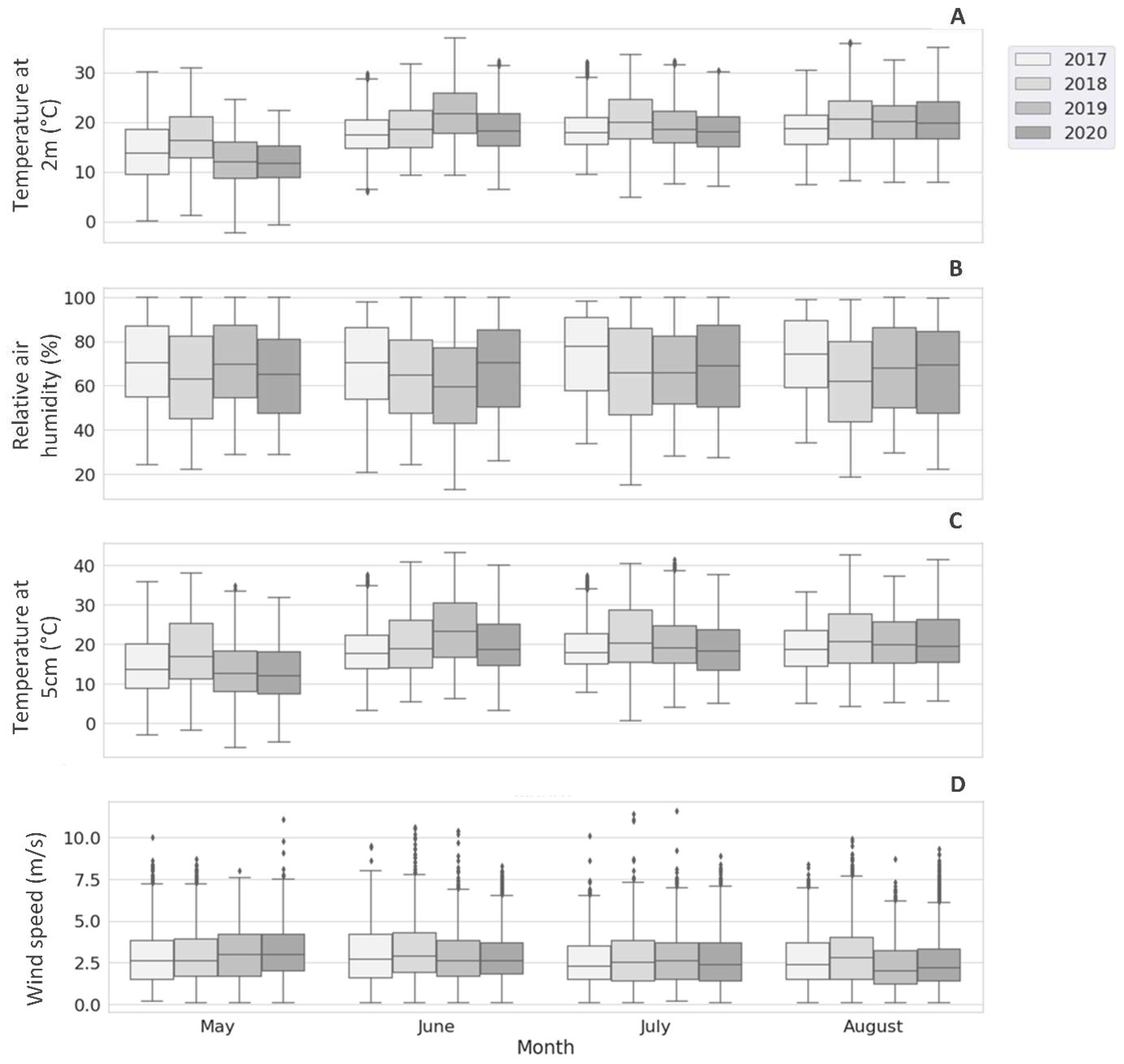
The experiment study site is located at the Leibniz Centre for Agricultural Landscape Research (ZALF), in Müncheberg, Germany (52°30′57.55″ N, 14° 7′22.27″ E, 59 m). The study area is characterised by high temperatures during late spring and summer, with frequent early-summer drought periods. For the period from 1981 to 2010, the mean annual air temperature was 9.1 °C and summer temperatures were 17.6 °C. The mean annual precipitation in this period was 553 mm, and the mean summer precipitation was 166 mm. The site includes fields planted with soybean for this experiment. Field experiments took place from 1 August to 1 September 2020. During the years 2017–2019, the mean annual precipitation in this area was 476.1 mm, and the mean air temperature was 10.6 °C; during the warm season (i.e., May, June, July, and August), the mean temperature was 18.3 °C. The mean annual sunshine duration was 1055.5 h. A comparison of the weather parameters (air temperature and relative humidity at 2 m height, along with soil surface temperature at 5 cm and wind speed) during the summer of the years 2017 to 2020 are presented in Figure 1.

In our experiment, the initial stage and part of the development stage of the soybean occurred in July, when the crops’ canopies nearly reached their full extent; the crops experienced the rest of their development, the middle and late-season stages of growth, by the end of August. We considered both crops in their late development and the mid-season stages of their growth in our study.

The ground was even and the soil had a sandy texture (Eutric Cambisol). The groundwater table was 12 m below the surface, and no drainage system was installed. The experiments were conducted in one experimental block of 220 m² for the soybean fields under irrigation and non-irrigation. Irrigation areas of about 1.3 ha were watered by several sprinklers. These sprinklers covered an area of 84 m × 3 m.

The irrigation schedule was based on a schedule developed at Hochschule Geisenheim University (Geisenheim, Germany) for both horticulture and field-crop agriculture [28]. Irrigation was based on the cumulative daily water deficit between precipitation and the specific crop potential evapotranspiration (PET). PET can be determined according to the Penman–Monteith equation or based on the reference crop approach proposed by the Food and Agricultural Organization of the United Nations (FAO) [29]. This experiment used the Penman–Monteith equation. The total irrigation water amount of the experiment was 120 mm. The amount of water for each irrigation was approximately 20 mm for half of each plot.

Table 1. Irrigation dates and depths during the growing stages, August 2020.

Crop	Soybean
Date & time	4 August 12:58:00	5 August 6:34:00	11 August 11:02:00	14 August 9:48:00	20 August 10:23:00	26 August 6:31:00
Depth (mm)	20	20	20	20	20	20

summarises the irrigation date and depth of the water for each research field during the development, middle, and late season of the growing stage.

2.1.1. Micrometeorological Observations

During the experimental period, when soybean was in the developmental and mid-season stages of its growth, the crop height changed rapidly. The experimental sites were equipped with sensors for recording the temperature and relative air humidity above (120 cm above the ground) and under each crop’s canopy (on the ground). The canopy-air temperature of the crop was obtained through double points on two sides of each plot with irrigated and non-irrigated features. Air temperature and relative air humidity of the canopy (above and beneath) were processed every 1 min by a data logger. A weather station was located 150 m to the north of the experimental plots, which recorded meteorological variables including air temperature, relative air humidity, wind speed, and air pressure (at 2 m above ground) at 10-min intervals.

The data logger (TFD 500; Temperatur–Feuchte–Datenlogger) was attached to wooden stakes located directly above the canopy (120 cm from the ground, Figure 2) to measure the temperature and relative air humidity (RH) of the canopy with 1-min resolution. Next to each stake, there was another data logger on the ground to record data beneath the crop’s canopy. The sensors have a precision of ±0.3 °C for temperature and ±3.0% for RH. Sensors were shielded by two layers of white plastic bowls with pores around the wall to prevent direct radiation influence whilst still ensuring ventilation. To account for any spatial variability of temperature and humidity above and below the canopy, four locations were set up 3.8 m apart lengthwise and 10 m apart by width in each representative plot (Figure 2).

2.1.2. Ancillary Data

In this experiment, we considered leaf area index (LAI) as one of the few variables that describe the distribution of optical properties of the canopy structure. The LAI is defined as integrating the leaf area density over the canopy height [30].

Leaf area index (LAI) was measured indirectly, using the SS1 SunScan Plant Canopy Analysis System (DeltaT Devices, Cambridge, UK). These LAI measurements took place between July and August on a weekly basis. Two plots, each with two irrigated and non-irrigated subplots, were demarcated on the soybean field. For each sensor, two additional points near the sensor were randomly measured in the field. Measurements were made, generally on bright days, during early July and late August. The measurements were used specifically to support the analysis for determining the growth stage of the soybean. This measurements later in this study helped us to detect the different growing stages of the soybean. Besides this, the canopy temperature was monitored by a thermal imaging camera (Komerci ELEKTRONIKHANDEL Wärmebildkamera HT-18, München, Germany) to provide essential information about both the water stress and growing stages of the soybeans in this study.

The thermal imaging camera recognises temperature differences, localises them precisely, and documents them by simultaneously recording digital and infrared images. It combines infrared thermal imaging technology (infrared sensor with 220 × 160 px) with surface temperature measurement in real time. The images, with a resolution of 35,200 pixels, have an accuracy of 2 K on a scale from −20 °C to 300 °C.

2.2. Modelling the Air Temperature Differences under Adiabatic Processes

This part of the study, the equation recommended in the FAO-56 Guidelines [31] is used to estimate reference crop evapotranspiration based on climate data at ten-minute intervals. The Python “Pyeto” library [32] was used to calculate meteorological parameters from climate data, which were then used to calculate the reference evapotranspiration. The FAO expressed the “full form” of the Penman–Monteith equation as follows:

$$ET=\frac{\mathrm{\Delta }\left(R_n-G\right)+{\rho }_a{c}_p\frac{\left(e_s-e_a\right)}{r_a}}{\left(\mathrm{\Delta }+\gamma \left(1+\frac{r_s}{r_a}\right)\right){\rho }_w\lambda }$$

(1)

Nevertheless, the only factors affecting reference evapotranspiration are climatic parameters, and the Pyeto library provides numerous functions to estimate missing meteorological data. Here, we applied the measured air temperature and relative humidity in the constant height above and within the soybean’s canopy to estimate its evapotranspiration. The energy for evaporation comes from the sensible and latent heat that makes water evaporate from the soil and migrate to the air-water content. Through this adiabatic process, the specific enthalpy remains constant; the sensible air temperature is reduced and is compensated by latent heat gain. This study considers the area under the canopy’s ambient as a system in which no heat or mass can be transferred out of the canopy. The impacts of wind below the canopy would be negligible compared to those above the canopy.

The specific enthalpy of moist air is a function of temperature and the mass of water vapour per unit of dry air:

$$h=1.006T+x\left(1.86T+2501\right),$$

(2)

where $h$ is the specific enthalpy [kJ kg^–1], $T$ is the air temperature [°C], and $x$ is the mass of water vapour in the given air volume [kg kg^–1]. The maximum mass of water vapour in the air depends on the of the air vapour temperature, which is estimated by the saturation pressure of water vapour at the given temperature [33].

$$p_S\left(T\right)=0.6108\times exp\left(\frac{17.27\times T}{T+237.3}\right)$$

(3)

$$x=0.622\phi p_s\frac{\left(T\right)}{\left(p-\phi p_s\left(T\right)\right)}$$

(4)

where $p_s$ is the saturation vapour pressure, $p$ is the atmospheric pressure of moist air, m_WS is the maximum saturation humidity ratio of air [kg kg^–1] and φ is relative humidity (%).

Under an adiabatic process, the enthalpy remains constant. Since the enthalpy is a function of temperature and mass of water vapour, the water mass increases after evapotranspiration (Equation (1)). To maintain the equilibrium of the equation (Equation (5)), the air temperature after evapotranspiration (T_c) must decrease.

$$h\left(T,x\right)=h\left(T_c,x+ET\right)$$

(5)

The Molliar diagram [34] is an ideal tool to evaluate air conditions as well as changes in air conditions. It illustrates the state of the adiabatic process before and after evapotranspiration (Figure 3).

During each irrigation period, the water content of the air will increase, and the mass of water within the boundaries of the closed system can increasingly reduce the ambient temperature. Under the canopy, with no water stress from the soil, the additional water due to evaporation increases the air-water content and causes a reduction in air temperature due to the previous adiabatic condition. Modelling this process to estimate T_c (Equation (5)) is feasible as long as the crop has no water stress (e.g., in the irrigated area of the field). In this experiment, we used measured air temperature and relative air humidity under the crops’ canopies in both irrigated and non-irrigated areas. The measured values in the non-irrigated areas were used as model inputs to simulate air temperature changes in the irrigated area (T_c). We were then able to compare the results of the model to the measured values from the irrigated areas to evaluate the accuracy of the model.

The experiment started after the crops had already passed this stage and started their development stage. During the respective development stage, the results of the model were only investigated for the warmest hours, when the temperature started to rise (10:00) in the morning and started to decrease in the evening (20:00). To improve the selection of the warming hours, we also considered the largest discrepancy of the relative air humidity for both irrigated and non-irrigated areas during this period.

The statistical analysis was conducted using the differences in the diurnal temperature observed in the field and temperature simulated by the model at a resolution of ten minutes. To evaluate the model results, we used statistical indexes, mean absolute error (MAE), and coefficient-of-determination metrics (also known as R-squared values). High R² values and low MAE values would demonstrate the acceptable performance of the model, indicating that the model simulations of a predefined thermodynamic process were close to the actual observations.

3. Result

3.1. Above the Canopy

The recording of data above the canopy began on 1 June, the initial stage of growth (ground cover of less than 10%), and continued until the end of August. From that data, the six days of irrigation were omitted as they did not meet the predefined experimental conditions. In the resulting data set, the average temperature in the irrigated site was 0.3 K lower than in the rainfed site. Our model simulation showed 0.2 K differences. During the growing stage, when the crops’ canopy had developed, the average diurnal air temperature in both areas increased by 3.2 K in the field, but the difference was relatively stable (0.2 K), while the model estimated a 0.4 K increase.

The wind speed during the recording period was highly variable and was generally in the range of 2.6 m s⁻¹ in the afternoon and 3.7 m s⁻¹ in the morning. This is considered a “light breeze” according to the Beaufort wind scale (see Figure S1 in the supplementary data for more details). The model results for MAE and R2 for both development and mid-season stages are presented in

Table 2. The performance indicators of R² and MAE in evaluating the model predictions of the temperature above the canopy of an irrigated soybean crop during the middle and late-season stages.

Growing and Mid-Season Stage			Late-Season Stage
Date	R2	MAE[K]	Date	R2	MAE[K]
1 August 2020	0.93	0.61	15 August 2020	0.95	0.52
2 August 2020	1.00	0.11	16 August 2020	0.90	0.56
3 August 2020	1.00	0.13	17 August 2020	0.98	0.31
4 August 2020	0.96	0.31	18 August 2020	0.93	0.27
5 August 2020	0.91	0.57	19 August 2020	0.99	0.17
6 August 2020	0.91	0.70	20 August 2020	1.00	0.10
7 August 2020	0.99	0.32	21 August 2020	0.99	0.18
8 August 2020	0.99	0.31	22 August 2020	0.98	0.26
9 August 2020	1.00	0.23	23 August 2020	0.99	0.17
10 August 2020	1.00	0.09	24 August 2020	1.00	0.08
11 August 2020	0.93	0.62	26 August 2020	0.94	0.37
12 August 2020	0.88	0.75	27 August 2020	0.98	0.28
13 August 2020	0.96	0.53	28 August 2020	0.99	0.30
14 August 2020	0.99	0.19	29 August 2020	0.99	0.20
			30 August 2020	0.99	0.43

individually, and in more detail in the supplementary material (Table S1).

During the development and mid-season stages of growth, the model simulations were slightly different on average, with MAE = 0.3 K and R² = 0.98. The model had the same performance during the late-season stage of growth. In general, the average diurnal temperatures above the canopy in the middle and late season stages were 30.8 °C and 25.3 °C, while the model estimations were 30.3 °C and 25.0 °C respectively.

Before the first irrigation, the average temperature at the irrigated site during the hottest hours was 0.2 K lower than at the non-irrigated site. The first irrigation round included two irrigation times; one was at midday on 4 August, and another was in the early morning on 5 August (Figure 4). In the five days following until the second irrigation, the recorded temperature above the canopy showed 0.1 K cooler values than the non-irrigated treatment; however, the model estimated a cooling effect of 0.3 K on the irrigated site.

During the mid-season stage, with three rounds of irrigation, the average air temperatures above the canopy in the irrigated and rainfed sides were 30.6 °C and 30.8 °C, respectively. The model estimated 0.5 K lower in the irrigated areas with a medium accuracy (MAE = 0.3 K and R² = 0.98). Throughout the irrigation round, relative humidity (RH) above the canopy in the non-irrigated areas barely changed compared to the non-irrigated ones—a maximum of 3% and a minimum of 0.5%.

3.2. Under the Canopy

There were no measurements below the canopy during the initial stage of growth. The data under the canopy was recorded in August when the crops had entered their development, middle and late-season stages. On 4 and 5 August, the crops had their first and second irrigations with the same amount of water (20 mm). Before the first irrigation in this stage, the average diurnal temperature under the canopy was 3.1 K cooler in the irrigated sites, while the model simulation was 3.9 K. The irrigation regularly took place every four to five days. In days with irrigation, the crops’ ET was influenced by the additional water. Therefore, data from those days were omitted from our data set. In the resulting data, the average diurnal temperature differences in the irrigated area during the middle and late-season stages were 3.9 K and 2.7 K lower than the rainfed area, while the model estimations forecasted 4.9 K and 3.3 K, respectively. The average relative humidity of each period before irrigation changed between 5.7% and 14.4%. The performance of the model is presented in

Table 3. The performance indicators R² and MAE evaluate the model predictions of the temperature above the canopy of an irrigated soybean crop during the middle and late-season stages.

Growing and Mid-Season Stage			Late-Season Stage
Date	R2	MAE [K]	Date	R2	MAE [K]
1 August 2020	0.67	2.31	15 August 2020	0.72	1.57
2 August 2020	0.88	0.56	16 August 2020	0.75	1.84
3 August 2020	0.88	0.46	17 August 2020	0.94	0.74
4 August 2020	0.51	2.26	18 August 2020	0.73	0.51
5 August 2020	0.17	4.29	19 August 2020	0.96	0.50
6 August 2020	0.60	2.31	20 August 2020	0.54	1.93
7 August 2020	0.93	0.77	21 August 2020	0.75	1.62
8 August 2020	0.94	0.81	22 August 2020	0.93	0.33
9 August 2020	0.95	0.78	23 August 2020	0.75	1.21
10 August 2020	0.97	0.58	24 August 2020	0.90	0.83
11 August 2020	−0.16	4.97	26 August 2020	0.87	0.26
12 August 2020	0.18	5.73	27 August 2020	0.98	0.27
13 August 2020	0.48	3.52	28 August 2020	0.99	0.27
14 August 2020	0.94	0.30	29 August 2020	0.97	0.36
			30 August 2020	0.97	0.39

.

However, the recorded data in the field during the hottest hours before the first irrigation indicated differences of 3.1 K, while model results indicated 4.0 K. The model performance for days without irrigation was high (R² = 81.2% and MAE = 1.1 K). Before the second irrigation, the observed and simulated differences of both sides were 4.0 K and 4.5 K, respectively (R² = 96.1% and MAE = 0.7 K). Before the last irrigation in the mid-season stage on 15 August, the values for both observation and simulation were 4.8 K and 6.5 K, respectively (R² = 71.0% and MAE = 1.8 K).

In general, the model’s performance on days with irrigation was lower than on the days without irrigation (on average R² = 51.0%, MAE = 2.3 K) (see Table S2 for more details). For days with no irrigation, the air temperature simulated by the model was between 0.06 K and 1.6 K lower than the air temperature observed in the field (R² changed in the range of 71.0% to 96.0% and MAE changed in the range of 0.7 K to 1.8 K).

Figure 5 shows the results of the estimated temperature and humidity compared to the recorded data in the irrigated area for the days between the first and second irrigations (for the whole irrigation period, see Figures S2–S5 in the Supplementary Material).

3.3. LAI and Thermal Images

Here, results from the LAI helped us to recognise different stages of the crops in the field, and the thermal images could prove that the impacts of the cooling effect of crops in the irrigated and rainfed areas correspond to the crop’s stage of growth. The average LAI in the areas with regular irrigation and no water stress were higher (1.9) than in the non-irrigated areas (0.6), see

Table 4. The average measured LAI at four points (irrigated and non-irrigated; soybean) in the field. The LAI for each crop represents the average of two points that were both located on one side of the field.

Date	Not Irrigated	Irrigated
4 August 2020	1.8	2.4
11 August 2020	1.2	1.8
19 August 2020	1	1.6

and

Table 5. The average measured crop height [cm] at four points (irrigated and non-irrigated; soybean) in the field. The crop height for each point represents the average of three other points around the point.

Date	Not Irrigated	Irrigated
4 August 2020	47.8	60.5
11 August 2020	48.7	64.8
19 August 2020	59.5	60.3

. On 4 August, the soybean crop passed the initial stage and began the mid-season stage, when the crop’s canopy had its maximum level of development, and the LAI reached its highest value. On 15 August, the crop entered the late-season stage, when the LAI of the soybean had already decreased in both irrigated and non-irrigated areas (Table 5).

In addition to the LAI of the soybean crop under the no-water stressed condition, the height of the crop decreased after passing the developmental stage on 15 August (Table 5).

The absolute temperature of the soybean crop captured by thermal camera on the irrigated area during the initial and mid-season stages was 1.1 K and 2.5 K lower than in the other area. On 19 August, one of the days in the late-season stage, this difference fell to 0.3 K (

Table 6. The average absolute temperature [°C] from pictures captured using the thermal camera at four points (irrigated and non-irrigated; soybean). The value for each point represents the average of three to six absolute points around the sensors.

Date	Not Irrigated	Irrigated
31 July 2020	22.6	21.5
4 August 2020	26.5	24.0
18 August 2020	22.1	21.8
26 August 2020	22.9	21.1

).

Details of the measured LAI, crop heights, and absolute temperature captured by the thermal camera are provided in the supplementary material (Tables S3–S5) individually for all spots for both areas (with and without irrigation).

4. Discussion

4.1. The Cooling Effect above the Canopy

Converting natural vegetation to irrigated agriculture can have a profound impact on local temperature, specifically on the average and maximum temperature during the warm months [35]. Only a few works have evaluated the physical–mathematical model and dynamic simulation for calculating ET_c in high resolution along with the main influencing parameters that have to be considered. Moreover, finding suitable equipment and methodologies are other obstacles for long-term measurements of the cooling effect [36].

This study applied a physical–mathematical method based on a specific thermodynamic process to estimate the confounding trend of temperature under and above the soybean’s canopy during the warm period between two irrigation practices. During the growing stage, the model performed more poorly and predicted lower differences the closer it came to irrigation events. In other words, the differences between observed and simulated temperatures were high during times of irrigation. This trend recurred in the first two days after irrigation, but it receded in the following days when no additional water existed in the air.

The model results above the canopy during the initial and mid-season stages were quite the opposite. In the initial stage, the vegetation cover was less than 10% and both areas were under quite similar conditions. The air above the canopy played a role as an adiabatic system, in which energy remained contained. The model performance for this stage of growth was quite good. The canopy-air temperature was influenced by wind, radiation, and the height of sensors. As a consequence, the model simulation can explain only a part of the cooling.

In the next growth stage, the vegetation cover in the irrigated areas became denser and higher (Table 4 and Table 5), which influenced the canopy’s temperature. The temperature differences caused air movement specifically on a small scale such as our plot, in addition to the existing light breeze in the region (Figure 1). The model indicated a negligible cooling effect above the canopy at the field scale when we considered the atmosphere above the canopy as an adiabatic system.

4.2. The Cooling Effect below the Canopy

In spite of numerous studies that have considered the cooling effects of irrigation on the canopy level, only a few specifically explored evaporative cooling below and above the canopy. Canopies prevent solar radiation from reaching the ground, thus reducing the heat storage underneath, and importantly the intercepted energy increases the latent heat flux somewhat. This reduces the air temperature during the daytime. At such a fine scale (i.e., in the field), any explanation of the below-canopy cooling effect needs to incorporate biological, micrometeorological, and edaphic factors [20]. Our study only considered micrometeorological factors, rather than biological and soil factors.

Effective physical control of irrigation depends on the possibility of estimating transpiration rates, which can be estimated from contemporary weather data [37]. In this study, irrigation helped to keep the soil wet enough and ensure that water supply was never a limiting factor in crop growth. Unlike the negligible cooling effect above the canopy during the middle and late-season stages of growth (0.2 K to 0.5 K, respectively), the cooling effect under the canopy was estimated to be 4 K to 5 K for both stages. In principle, the model showed no acceptable performance during the experimental period, either on days with irrigation (or one day after that) or on rainy days. In those days, additional water was transferred into the system. The error of the model on days without irrigation is due to water being intercepted on the plant surface from previous irrigation events. In this experiment, the interception error impeded the model result on the respective day of irrigation and the day after.

The maximum temperature changes occurred on days with irrigation (or the following days) that did not follow the aforementioned hypothetical condition. The model performed the poorest on those days. The minimum cooling effect occurred when the air-water vapour capacity in both the irrigated and non-irrigated areas were similar. This condition usually occurred a long time after the individual irrigation events, and the model performance consequently improved.

4.3. Model Limitations

Different kinds of plants may have different transpiration rates, which are also influenced by crop characteristics, environmental aspects, and cultivation practices. In the initial stage of growth, soil loses lots of water because of relatively little coverage of the soil surface; however, once the crop is well-developed, transpiration becomes the main process [29,38]. This amount of water increases the air-water content under the canopy, which the model does not account for when estimating the temperature.

The vegetation cover and ground cover changed continuously during the growing period, which meant that the crop coefficient (K_c) varied. The crop coefficient is represented in the crop coefficient curve as the transpiration component of ET. Three values are required for K_c to describe and construct the crop coefficient curve: those during the initial stage (K_{c ini}), the mid-season stage (K_{c mid}), and at the end of the late-season stage (K_{c end}) [29]. In this study, we applied only K_c of the mid-season stage for the mid-season and late-season stages of growth.

5. Conclusions

During the warm months of the year, and particularly in the hottest hours, the temperature above and under the canopy of soybean plants with an adequate water supply was cooler than non-irrigated areas at the plot scale. The nonlinear relationship of the vertical temperature gradient above and under the canopy is defined by a complex interaction of micrometeorological, biological, and soil-related factors. It is essential in landscape management to consider the feedback among vegetation, soil temperature, air temperature, and air-water content when designing a strategy to provide cooling services.

We introduced a physics-based model to estimate an evaporative cooling effect above and under the crop’s canopy. At the field scale, we were limited to using sets of meteorological data. Our results nevertheless serve to indicate how regular irrigation that prevents the risk of water stress for crops serves the ecosystem management at field scale, with knock-on effects for the soil ecosystem and biodiversity. With this model, we are now able to assess the potential cooling effect of crop irrigation as a possible contribution to a cooling-service design at the landscape scale. In this study, we applied the model to soybeans and it appears to perform well with that crop. We suspect that the model with its thermodynamic aspect would be generally applicable for other crop types, using their crop coefficient. While evapotranspiration is specific to the crop, the model as such can be used without specific changes to estimate the evaporative cooling effect.

References

1. Seneviratne, S.I.; Donat, M.G.; Pitman, A.J. Managing the Risks of Extreme Events and Disasters to Advance Climate Change. Intergovernmental Panel on Climate Change; Cambridge University Press: New York, NY, USA, 2012. [Google Scholar]
2. Arnell, N.W.; Lowe, J.A.; Challinor, A.J.; Osborn, T.J. Global and regional impacts of climate change at different levels of global temperature increase. Climate Chang. 2019, 155, 377–391. [Google Scholar] [CrossRef] [Green Version]
3. Fischer, E.M.; Schär, C. Future changes in daily summer temperature variability: Driving processes and role for temperature extremes. Clim. Dyn. 2009, 33, 917–935. [Google Scholar] [CrossRef]
4. Ruthrof, K.X.; Breshears, D.D.; Fontaine, J.; Froend, R.; Matusick, G.; Kala, J.; Miller, B.; Mitchell, P.J.; Wilson, S.; van Keulen, M. Subcontinental heat wave triggers terrestrial and marine, multi-taxa responses. Sci. Rep. 2018, 8, 1–9. [Google Scholar] [CrossRef] [PubMed]
5. Smith, M.D. The ecological role of climate extremes: Current understanding and future prospects. J. Ecol. 2011, 99, 651–655. [Google Scholar] [CrossRef]
6. Teskey, R.; Wertin, T.; Bauweraerts, I.; Ameye, M.; McGuire, M.A.; Steppe, K. Responses of tree species to heat waves and extreme heat events. Plant Cell Environ. 2014, 38, 1699–1712. [Google Scholar] [CrossRef] [PubMed]
7. IPCC. Climate Change: Impacts, Adaptation, and Vulnerability. Part A: Global and Sectoral Aspects. In Contribution of Working Group II to the Fifth Assessment Report of the Intergovernmental Panel on Climate Change; Cambridge University Press: Cambridge, UK; New York, NY, USA, 2014; 1132p. [Google Scholar]
8. Ainsworth, T.D.; Heron, S.F.; Ortiz, J.C.; Mumby, P.J.; Grech, A.; Ogawa, D.; Eakin, C.M.; Leggat, W. Climate change disables coral bleaching protection on the Great Barrier Reef. Science 2016, 352, 338–342. [Google Scholar] [CrossRef] [Green Version]
9. Dijkstra, J.A.; Westerman, E.L.; Harris, L.G. The effects of climate change on species composition, succession and phenology: A case study. Glob. Chang. Biol. 2010, 17, 2360–2369. [Google Scholar] [CrossRef]
10. Dunne, J.P.; Stouffer, R.J.; John, J.G. Reductions in labour capacity from heat stress under climate warming. Nat. Clim. Chang. 2013, 3, 563–566. [Google Scholar] [CrossRef]
11. Daryanto, S.; Wang, L.; Jacinthe, P.-A. Global Synthesis of Drought Effects on Maize and Wheat Production. PLoS ONE 2016, 11, e0156362. [Google Scholar] [CrossRef]
12. Rahman, M.A.; Hartmann, C.; Moser-Reischl, A.; von Strachwitz, M.F.; Paeth, H.; Pretzsch, H.; Pauleit, S.; Rötzer, T. Tree cooling effects and human thermal comfort under contrasting species and sites. Agric. For. Meteorol. 2020, 287, 107947. [Google Scholar] [CrossRef]
13. Rahman, M.; Armson, D.; Ennos, A. Effect of urbanization and climate change in the rooting zone on the growth and physiology of Pyrus calleryana. Urban For. Urban Green. 2014, 13, 325–335. [Google Scholar] [CrossRef]
14. Edmondson, J.L.; Stott, I.; Davies, Z.G.; Gaston, K.J.; Leake, J.R. Soil surface temperatures reveal moderation of the urban heat island effect by trees and shrubs. Sci. Rep. 2016, 6, 1–8. [Google Scholar] [CrossRef] [Green Version]
15. Zölch, T.; Maderspacher, J.; Wamsler, C.; Pauleit, S. Using green infrastructure for urban climate-proofing: An evaluation of heat mitigation measures at the micro-scale. Urban For. Urban Green. 2016, 20, 305–316. [Google Scholar] [CrossRef]
16. Findell, K.L.; Shevliakova, E.; Milly, P.C.D.; Stouffer, R.J. Modeled impact of anthropogenic land cover change on climate. J. Clim. 2007, 20, 3621–3634. [Google Scholar] [CrossRef] [Green Version]
17. De Frenne, P.; Zellweger, F.; Rodriguez-Sanchez, F.; Scheffers, B.; Hylander, K.; Luoto, M.; Vellend, M.; Verheyen, K.; Lenoir, J. Global buffering of temperatures under forest canopies. Nat. Ecol. Evol. 2019, 3, 744–749. [Google Scholar] [CrossRef]
18. Broadbent, A.M.; Coutts, A.M.; Tapper, N.J.; Demuzere, M. The cooling effect of irrigation on urban microclimate during heatwave conditions. Urban Clim. 2018, 23, 309–329. [Google Scholar] [CrossRef]
19. Biggs, T.W.; Scott, C.A.; Gaur, A.; Venot, J.-P.; Chase, T.; Lee, E. Impacts of irrigation and anthropogenic aerosols on the water balance, heat fluxes, and surface temperature in a river basin. Water Resour. Res. 2008, 44, W12415. [Google Scholar] [CrossRef]
20. Lobell, D.B.; Bonfils, C.J.; Kueppers, L.M.; Snyder, M.A. Irrigation cooling effect on temperature and heat index extremes. Geophys. Res. Lett. 2008, 35, L09705. [Google Scholar] [CrossRef]
21. Santamouris, M.; Ban-Weiss, G.; Osmond, P.; Paolini, R.; Synnefa, A.; Cartalis, C.; Muscio, A.; Zinzi, M.; Morakinyo, T.E.; Ng, E.Y.Y. Progress in urban greenery mitigation science–assessment methodologies advanced technologies and impact on cities. J. Civ. Eng. Manag. 2018, 24, 638–671. [Google Scholar] [CrossRef] [Green Version]
22. Hoelscher, M.-T.; Nehls, T.; Jänicke, B.; Wessolek, G. Quantifying cooling effects of facade greening: Shading, transpiration and insulation. Energy Build. 2016, 114, 283–290. [Google Scholar] [CrossRef]
23. Estoque, R.C.; Murayama, Y.; Myint, S.W. Effects of landscape composition and pattern on land surface temperature: An urban heat island study in the megacities of Southeast Asia. Sci. Total Environ. 2017, 577, 349–359. [Google Scholar] [CrossRef] [PubMed]
24. Mahmood, R.; Pielke, R.A., Sr.; Hubbard, K.; Niyogi, D.; Dirmeyer, P.A.; McAlpine, C.; Carleton, A.M.; Hale, R.; Gameda, S.; Beltrán-Przekurat, A. Land cover changes and their biogeophysical effects on climate. Int. J. Clim. 2013, 34, 929–953. [Google Scholar] [CrossRef] [Green Version]
25. Hou, H.; Estoque, R.C. Detecting Cooling Effect of Landscape from Composition and Configuration: An Urban Heat Island Study on Hangzhou. Urban For. Urban Green. 2020, 53, 126719. [Google Scholar] [CrossRef]
26. Coleman, R.; Stavros, N.; Hulley, G.; Parazoo, N. Comparison of Thermal Infrared-Derived Maps of Irrigated and Non-Irrigated Vegetation in Urban and Non-Urban Areas of Southern California. Remote Sens. 2020, 12, 4102. [Google Scholar] [CrossRef]
27. Siebert, S.; Webber, H.; Zhao, G.; Ewert, F. Heat stress is overestimated in climate impact studies for irrigated agriculture. Environ. Res. Lett. 2017, 12, 054023. [Google Scholar] [CrossRef]
28. Paschold, P.-J.; Kleber, J.; Mayer, N. Geisenheimer Bewässerungssteuerung; Hochschule Geisenheim University: Geisenheim, Germany, 2010; pp. 1–7. [Google Scholar]
29. Allen, R.G.; Pereira, L.S.; Raes, D.; Smith, M. Crop evapotraspiration guidelines for computing crop water requirements. Fao Rome 1998, 300, D05109. [Google Scholar]
30. Weiss, M.; Baret, F.; Smith, G.; Jonckheere, I.; Coppin, P. Review of methods for in situ leaf area index (LAI) determination: Part II. Estimation of LAI, errors and sampling. Agric. For. Meteorol. 2004, 121, 37–53. [Google Scholar] [CrossRef]
31. FAO. Crop Evapotranspiration-Guidelines for Computing Crop Water Requirements-FAO Irrigation and Drainage Paper 56. 1998. Available online: http://www.fao.org/3/x0490e/x0490e00.htm#Contents (accessed on 6 April 2021).
32. Richards, M. PyETo Implements Methods for Estimating Evapotranspiration. 2015. Available online: https://pyeto.readthedocs.io/en/latest/overview.html (accessed on 24 November 2021).
33. Engineering ToolBox. 2004. Available online: https://www.engineeringtoolbox.com/enthalpy-moist-air-d_683.html (accessed on 31 July 2021).
34. Mankonen, A.; Kaikko, J.; Vakkilainen, E.; Sergeev, V. Thermodynamic analysis of a condensing evaporator in an evaporative gas turbine cycle. MATEC Web Conf. 2018, 245, 07007. [Google Scholar] [CrossRef]
35. Kueppers, L.M.; Snyder, M.; Sloan, L.C. Irrigation cooling effect: Regional climate forcing by land-use change. Geophys. Res. Lett. 2007, 34, 1–5. [Google Scholar] [CrossRef] [Green Version]
36. Casconea, S.; Comab, J.; Gaglianoc, A.; Pérezd, G. The evapotranspiration process in green roofs: A review. Build. Environ. 2018, 147, 337–355. [Google Scholar] [CrossRef]
37. Penman, H.L. The physical bases of irrigation control. Proceedings of the Report of the 13th International Horticultural Congress, Adelaide, South Australia, 1952; pp. 1–13. Available online: https://repository.rothamsted.ac.uk/download/c8d6335630949fbe87fac367fbed53ce2dce2f523b7b179092b08badde2b3d9c/1719129/1817_001.pdf (accessed on 24 November 2021).
38. Zotarelli, L.; Dukes, M.D.; Romero, C.C.; Migliaccio, K.W.; Morgan, K.T. Step by Step Calculation of the Penman-Monteith Evapotranspiration (FAO-56 Method); Institute of Food and Agricultural Sciences, University of Florida: Gainesville, FL, USA, 2014; pp. 1–14. [Google Scholar]
Figure 1. Hourly air temperature at 2 m (A), relative air humidity at 2 m (B), soil surface temperature at 5 cm (C), and wind speed (D) for the years 2017, 2018, 2019, and 2020.
Water 14 00319 g001
Figure 2. The location of each sensor in the field (left). All sensors located at a height of 1.2 m.
Water 14 00319 g002
Figure 3. Part of the Molliar diagram illustrating the temperature after evapotranspiration under an adiabatic process. The curved lines describe relative humidity as a percentage; the scale ranges from 0% up to the saturation line of 100% relative humidity. The diagonal lines describe the specific enthalpy.
Water 14 00319 g003
Figure 4. The air temperature (A) and relative air humidity (B) at a ten-minute resolution between 10:00 and 21:00 above the canopy during the days between the first and second irrigation rounds.
Water 14 00319 g004
Figure 5. The air temperature (°C) (A) and relative air humidity (%) (B) at a ten-minute resolution between 10:00 and 21:00 below the canopy for the days between the first and the second irrigation event.
Water 14 00319 g005