Abstract
Mariculture areas are an important non-renewable natural resource and continuously improving their efficiency is important for increasing mariculture output and adjusting its structure. The aim of this study was to measure the mariculture area production efficiency (MAPE) considering undesirable outputs, further analyze its spatiotemporal disparities, and analyze the reasons for the differences observed during the period from 2008 to 2019. The super-efficiency Engel–Blackwell–Miniard (S-EBM) model and global Malmquist–Luenberger (GML) index was selected to analyze the technical efficiency and productivity of MAPE from both the static and dynamic aspects, and the Theil index was used to decompose the regional differences. The results showed that the MAPE showed fluctuation and an increasing trend overall; the production efficiency and technical progress showed a fluctuating rising trend, and technical progress had a significant driving effect on the production efficiency; and intra-regional differences were the main factors that cause the differences in MAPE. The findings suggest the increase of scientific and technological investment in mariculture, changes in mariculture methods, the establishment of environmental monitoring centers in mariculture areas, and the sharing of information technology between regions to achieve sustainable development.
1. Introduction
The ocean is a major component of the global life support system and a valuable resource that helps to achieve the sustainable development of human society [1]. With the rapid increase of the global population, environmental pollution, and shortages of resources, food problems are becoming increasingly serious [2,3]. Due to economic development and the improvement of living standards, people are not satisfied with merely solving the problem of food quantity, but are also paying more attention to the pursuit of high-quality food [4,5]. Therefore, many coastal countries have focused their strategic vision on the ocean, and protein extraction from the ocean has become a hot industry in relation to solving food security issues at present and in the future [6]. According to the Global Aquaculture Production database, the global mariculture production in 2019 reached 57,872.179 kilotons. Although the current growth rate has slowed down, production has always maintained a growth trend. The mariculture production in China ranks first in the world and is developing rapidly, increasing from 10 kilotons in 1950 to 36,403.631 kilotons in 2019, accounting for 3.17% and 62.9% of the world’s mariculture production, respectively. Therefore, as a powerful mariculture country, China’s research on mariculture is of great significance, and can provide guidance and reference for other coastal countries or regions to develop and utilize mariculture sea areas.
In recent years, China’s mariculture is facing severe challenges; for instance, the overall mariculture area has decreased year by year, and the ecological environmental pollution in mariculture areas has become increasingly serious [7]. According to the Report on the State of the Fishery Eco-Environment in China, from 2015 to 2018, the emissions of the major mariculture areas in China exceeded standards to a large extent, with inorganic nitrogen and active phosphate exceeding 52% in the detected area [8]. This development reduces the productivity of polluted sea areas and also affects the sustainable development of mariculture. In this context, continuously improving mariculture area production efficiency (MAPE) has become the key to increasing mariculture production and ensuring food security under the constraints of the marine ecological environment.
As the world’s attention to the ocean increases, China is also paying more and more attention to ocean research [9,10,11,12,13], and relevant studies have been conducted from the perspective of mariculture areas [14,15]. A mariculture area is defined as a non-renewable key resource element for mariculture and seafood production is similar to grain production [16]. That is, grain is produced using cultivated land resources, whereas seafood is produced using mariculture areas. The mariculture area is equivalent to the cultivated land in grain production, and the production processes are similar. China is a country with a large population, and since ancient times, agriculture has been the foundation of the country [17,18]. China’s cultivated land research has been more in-depth [19,20,21], and relatively speaking, the number of specific studies on mariculture areas is relatively small, and the research content relating to the ocean primarily focuses on the entire marine economy or marine industry [22,23,24,25]. Collectively, these studies put more emphasis on the importance of cultivated land development and utilization, and the whole sea area, but no previous study has considered the use of mariculture sea areas from the perspective of sea area resources.
Therefore, to fill the knowledge gap noted above, China’s east coast was selected as the study area in this research to evaluate the MAPE of China from 2008 to 2019 and further explore its temporal and spatial disparities. This study is based on the existing research methods, considering the undesirable output of mariculture areas, which is a multi-output situation, using the super-efficiency Engel–Blackwell–Miniard (S-EBM) model and the global Malmquist–Luenberger (GML) index to measure and analyze the technical efficiency and productivity of MAPE from both the static and dynamic perspectives. The main aims of this study were to measure the MAPE, to further analyze its temporal and spatial differences, and to analyze the reasons for the differences through the Theil index. The results of this research will be helpful for improving the production efficiency and realizing the voluntary and sustainable development of mariculture areas, and may provide guidance for the development and utilization of sea areas and relevant decision-making.
The remainder of this paper is organized as follows. In Section 2, we briefly review the existing literature on mariculture, focusing on production efficiency and methods. Section 3 introduces the methodology used for evaluating and analyzing MAPE. Section 4 presents the input and output indicators, as well as the data processing methods. The results of the empirical study on the China’s east coast MAPE over 2008–2019 are presented in Section 5, followed by the conclusions and discussion in Section 6.
2. Literature Review
2.1. Research on Mariculture
The research literature on mariculture mainly focuses on mariculture development, policy, efficiency evaluation, etc. Salayo et al. [26] defined mariculture in the Philippines as the cultivation of finfish, shellfish, seaweed, and other commodities in cages, pens, stakes, and rafts in the marine environment and assessed the biophysical and socio-economic background of mariculture. Yu et al. [6] analyzed the evolution of China’s mariculture policy and divided it into three stages: the mariculture production period, mariculture integrated management period, and mariculture sustainable development period, and analyzed the characteristics of the evolution of China’s mariculture policy accordingly. Yu et al. [27] used a measurement model based on over-relaxation and the GML index to measure the mariculture efficiency scores and their changes in nine coastal provinces of China from 2004 to 2016, and found that the efficiency of mariculture had increased by 6.45% from 2004 to 2016, and technological progress was the main driving force.
2.2. Research on Methods of Efficiency
Efficiency evaluation methods are a hot topic in the efficiency field and there are generally three methods for measuring efficiency: the single-index method [28,29], stochastic frontier analysis (SFA) [30,31], and data envelope analysis (DEA) [32,33,34,35]. Since DEA and SFA methods are currently used more commonly, the following literature mainly focus on efficiency evaluation approaches using these two methods.
The SFA method uses the construction of a production function to construct the production frontier and the deviation is decomposed into technical inefficiency and random error [36]. The result is less affected by the specific features of the sample and is more reliable and stable. In recent years, SFA has become popular in efficiency evaluation. Shabanzadeh-Khoshrody et al. [37] used the Tornqvists–Theil (TTP) index, SFA, and the matching method to analyze the effects of the Baft dam construction on the efficiency and productivity of downstream agricultural land. Van Nguyen et al. [38] examined the sensitivity of technical and scale efficiency estimates in stochastic frontier analysis, using data from an Australian fishery. Wang et al. [39] used the SFA model to evaluate the performance of soil and water conservation in consideration of changes in local environmental managers.
Different from the SFA parameter method, DEA is a non-parametric evaluation method, and the DEA method is mature in the study of efficiency measurement. Wang et al. [40] constructed a fully fuzzy DEA and used the large datasets of 264 Chinese cities over 2009–2018 to evaluate the urban circular economy. Some scholars have begun to pay attention to the spatiotemporal differences in production efficiency [41,42,43]. Given the increasingly severe environmental problems, some scholars have begun to focus on undesirable outputs [44,45,46]. Wang et al. [47] used the DEA model to calculate the ecological efficiency of China, considering undesirable outputs. Saber et al. [48] calculated the eco-efficiency for each of four impact categories (i.e., terrestrial, freshwater, and marine ecosystems, as well as human health) and analyzed differences in eco-efficiency between 200 paddy farms in Iran. Nabavi-Pelesaraei et al. [49] used the method of life cycle assessment (LCA) and DEA to measure the environmental efficiency of different systems and evaluated the possibility of the application of solar energy technology in the production of sunflower oil in Iran.
2.3. Research on Efficiency Measurements of Mariculture
From the perspective of efficiency measurements of mariculture, some scholars have used different methods to study this field. Singh et al. [50] used SFA to study the economic efficiency of aquaculture in southern Tripura. Nielsen et al. [51] used DEA to analyze the impact of the new environmental water purification system on the efficiency of freshwater aquaculture in Denmark. Ji et al. [52] and Wang et al. [53] used the economic loss of pollution as an undesired output and a DEA model to measure the efficiency of aquaculture and the mariculture industry in China. Vassdal et al. [54] used the Malmquist productivity index to measure the total factor productivity (TFP) of the marine salmon produced in Norway.
2.4. Literature Summary
At present, the efficiency evaluation of mariculture is a research hotspot, and there are several studies available for research. We classify and summarize these literatures and present a table summarizing the related studies (Table 1). Although the efficiency of mariculture has been studied, the production efficiency of the aquaculture area has not been explored to a large extent, and there is still a lack of comprehensive and effective evaluations. Mariculture research mainly focuses on qualitative analysis, whereas quantitative analysis on production efficiency measurement is rare. The methods used in these studies are singular, and previous studies have not considered the combination of static and dynamic methods when comprehensively considering environmental constraints. Thus, it is urgently required to develop a method for MAPE.

Table 1.
Summary of the related studies.
3. Materials and Methods
3.1. The S-EBM Model with Consideration of Undesirable Outputs
Currently, the methods for measuring efficiency primarily include SFA and DEA. The SFA model considers the effect of random errors on efficiency but relies on stricter assumptions and is mainly applicable to multiple inputs and single outputs. The DEA model is a non-parametric method that calculates the relative efficiency of a decision-making unit (DMU) by constructing the production frontier of the data and is the most commonly used among the two methods [55]. The traditional DEA model considers only the radial distance and ignores the influence of slack variables; therefore, it cannot measure efficiency by additionally considering undesirable outputs accurately [56]. In response to this problem, Tone [57] proposed the slacks-based measure (SBM) model, which takes into account the effects of slack variables on efficiency measurements, while avoiding the deviation caused by the difference in radial and angle distances and solving the high efficiency problem of the traditional DEA estimation approach. A disadvantage of this method is that it cannot handle a situation in which the input and output are both radial and non-radial. The Engel–Blackwell–Miniard (EBM) model was developed based on this model and can handle mixed radial situations (both radial and non-radial values) and calculate the non-radial values of inputs and outputs [58].
When the DEA model is used for analysis, there are often multiple DMUs that are evaluated as effective. Especially when the number of input and output indicators is large, the number of effective DMUs will increase. In the traditional DEA model, the maximum efficiency value is 1. At this point, the effective DMU efficiency value is equal, and it is difficult to further distinguish the level of DMU efficiency value. In order to solve this problem, Andersen et al. proposed a “super-efficiency model”, which can eliminate the evaluated DMU from the reference set, so the efficiency value of the evaluated DMU is obtained by referring to the frontier of the other DMU [59]. The effective DMU value is generally greater than 1, so the effective DMU can be distinguished. Therefore, in this paper we use the S-EBM model to measure the MAPE.
Taking provinces as DMUs, in this study we construct the set of production possibilities for MAPE, as shown in formula (1). Assuming that there are periods and DMUs , each DMU has m , and species of the input , the desirable output and the undesirable output , respectively. In Formula (1), λ is the weight of each DMU in establishing the set of production possibilities.
On this basis, the S-EBM model is constructed, and the model is expressed as follows [60]:
where is the objective function and is the number of DMUs; , , and represent the number of inputs, desirable outputs, and undesirable outputs, respectively; , , and represent the slack variables of inputs, desirable outputs, and undesirable outputs, respectively; , , and represent the weights of input indicators, desirable outputs, and undesirable outputs, respectively; is the planning parameter of the radial part; and is the key parameter.
3.2. GML Index
The S-EBM model proposed in this study can measure the MAPE and perform static analysis; however, it cannot measure the trend change of the efficiency value in the time series and cannot perform dynamic analysis [61]. However, the GML index is an improvement of the traditional Malmquist–Luenberger index, which makes it possible to compare the efficiency across time periods and can make up for the defects of the S-EBM model [62,63]. The GML index belongs to dynamic analysis, which can analyze the changes in TFP and the effects of technical efficiency and technological progress. Therefore, in this study we combine it with the GML index analysis method to analyze the production efficiency in different years. Therefore, based on the static analysis of MAPE conducted using the S-EBM model, in this study we further use the GML index to dynamically analyze the TFP of MAPE for different years. The GML index from period to period is expressed as follows:
where , , and represent the changes in input-output efficiency, technical efficiency, and technical progress from period to period , respectively. A value above 1 indicates an increase in production efficiency, and a decrease in efficiency otherwise.
3.3. Theil Index
The Theil index is an important method for measuring regional differences. It can decompose regional differences into intra- and inter-regional differences and measure the contribution rate of the two differences to the overall difference. Therefore, it not only reflects the evolution process of intra- and inter-regional differences, but also the main factors that cause the total difference [64]. The formulas are as follows:
where indicates the Theil index of MAPE, the intra-regional Theil index, the inter-regional Theil index, the efficiency of the -th province, the total efficiency of regions, the total efficiency of the -th region, the number of regions, and and represent the contribution rates of inter- and intra-regional differences, respectively.
4. Data and Variables
4.1. Variable Selection
MAPE reflects the production capacity of sea areas. In terms of input indicators, combined with the existing research and considering data availability, the input indicators include the resource input, labor input, capital input, fish fry, and feed inputs. The collected or constructed data are as follows:
(1) Resource input: The “breeding sea area” in the China Fishery Statistical Yearbook is selected as the variable for resource inputs.
(2) Labor input: The “labor engaged in marine aquaculture” in the China Fishery Statistical Yearbook is selected as the variable for the labor input.
(3) Capital input: The “capital deposit of mariculture” is selected. Since these data are not clearly stated in the Statistical Yearbook, the “capital deposit of mariculture” is estimated using the perpetual inventory method, based on Fan et al. [65]. The formula is as follows:
The capital deposit of the base year is:
where represents the capital deposit of the -th region in the period, the fixed investments, the depreciation rate, and the geometric mean of the fixed assets.
(4) Output: The output indicators include both the desirable and undesirable outputs. To better measure the MAPE and eliminate the impact of the differences in the aquaculture structure on desirable output, in this study we take the mariculture production value as the desirable output indicator and use 2008 as the base year to deflate the mariculture production value from 2008 to 2019. Undesirable output mainly refers to pollutants discharged during mariculture. Based on Ji et al. [66], the output of nitrogen (N), phosphorus (P), and chemical oxygen demand (COD) equivalent pollutants from mariculture are selected as undesirable outputs in this study. The specific calculation formula is as follows:
where represents the pollutant ( = , , or ) from mariculture production in the area, indicates the output of the -th seafood in the -th region, the proportion of the -th breeding method used in the -th region to produce the -th seafood type, the pollution production coefficient of the -th region using the -th breeding method to produce the -type seafood, the ratio of the -th breeding method to the total output, the equivalent pollutants in the -th area, and represents whether the 0 or 1 variable can be used.
4.2. Study Area
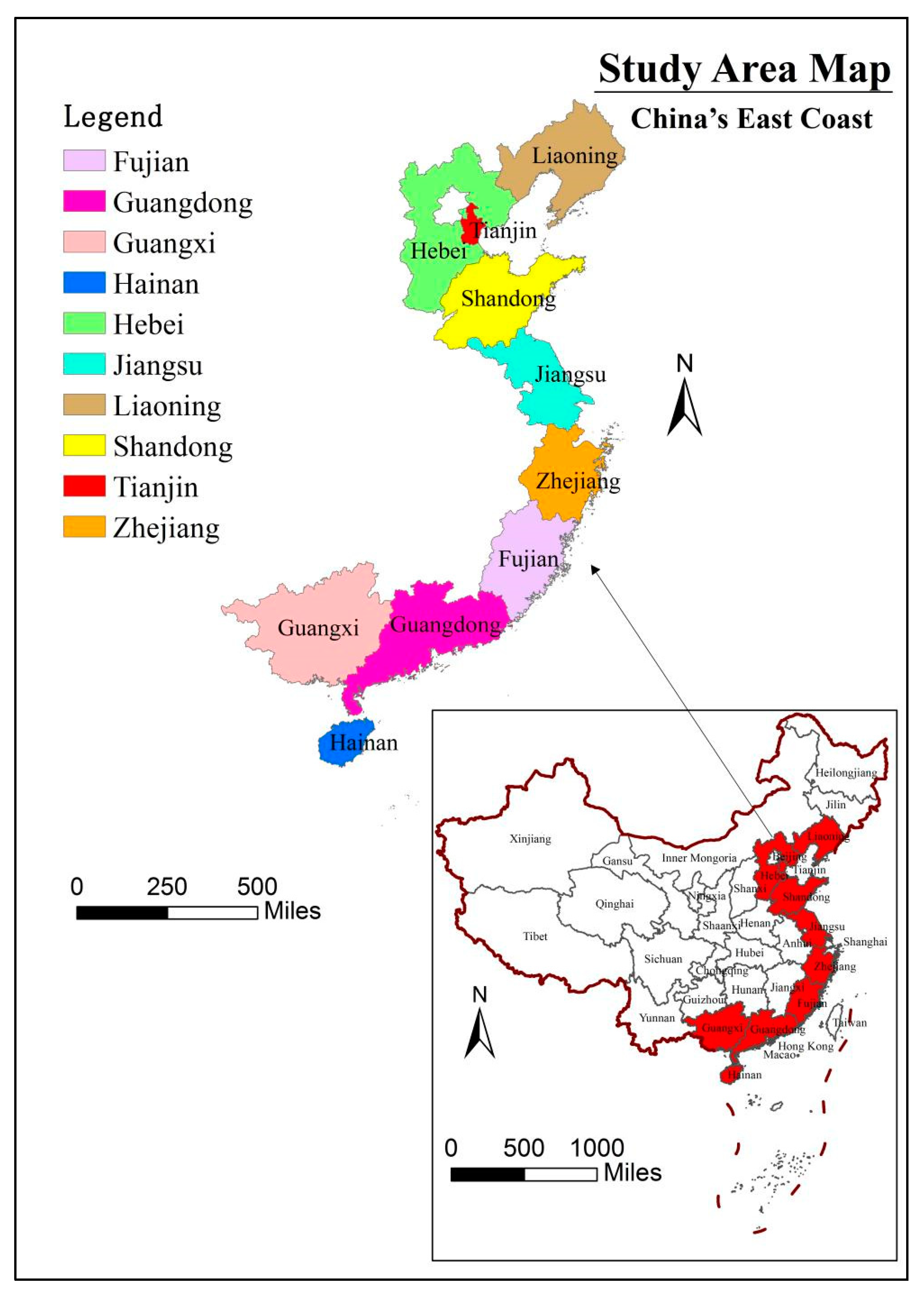
China’s east coast (18°10′–43°26′ N, 104°29′–125°46′ E) is located in eastern China, adjacent to the Bohai Sea in the north, the Yellow Sea and the East China Sea in the Middle East, the South China Sea in the south; facing Japan, North Korea, and South Korea across the sea in the north; Taiwan Province across the Taiwan Strait in the southeast; and Vietnam, Philippines, Brunei, and Malaysia across the sea in the south. In this study, we selected 10 coastal region as the sample: Liaoning Province, Hebei Province, Tianjin Municipality, Shandong Province, Jiangsu Province, Zhejiang Province, Fujian Province, Guangxi Zhuang Autonomous Region, Guangdong Province, and Hainan Province (Figure 1). Due to data availability and completeness, this study does not include Shanghai, Taiwan, Macau, and Hong Kong. As these areas have been engaged in mariculture for a long time, the 10 coastal region represent all the activities involved in China’s mariculture production, and the study of the production efficiency of their sea areas can fully reflect the overall MAPE situation.
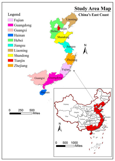
Figure 1.
Study area map.
4.3. Data Sources
To ensure integrity and uniformity of the data, the related data for 2008–2019 were calculated to determine production efficiency. All relevant data are from the 2009–2020 China Fishery Statistical Yearbook. In order to remove the effects of price changes, we set 2008 as the base year and adjusted the mariculture production value to a constant price. The descriptive statistics of the variables are shown in Table 2. As shown in Table 2, there are large differences in the input–output indicators of the 10 coastal regions.
Table 2.
Descriptive statistics.
5. Results
5.1. Statistic Analysis of MAPE
5.1.1. Temporal Disparity Analysis of MAPE
Using MaxDEA7 software, MAPE can be calculated using the S-EBM mode. See Table 3 for details. The efficiency is divided into four grades [67]: the low-efficiency area (efficiency within (0, 0.7)), lower-efficiency area (efficiency within (0.7, 0.8)), medium-efficiency area (efficiency within (0.8, 1)), and high-efficiency area (efficiency greater than or equal to 1). From Table 3, the spatiotemporal differences in the MAPE vary greatly, and a specific analysis is presented below.
Table 3.
Mariculture areas’ production efficiency.
According to the average value of MAPE from 2008 to 2019 (Table 3), the overall MAPE fluctuates and increases. The overall level of MAPE is relatively high, namely, in the medium–high-efficiency areas. In 2008, the efficiency was 0.947 and then increased continuously. From 2010 to 2013, efficiency was in a state of falling volatility, and then from 2014 to 2019, the average efficiency recovered and entered the high-efficiency area in 2019. Overall, the MAPE has generally shifted from a medium-efficiency area to a high-efficiency one. The reason for this is that the early stage of the study was at the beginning of the country’s advocacy of marine construction and marine development. As such, with the development of mariculture in various regions, the scale of mariculture continued to expand, and the maricultural area and capital investment increased rapidly, which promoted the MAPE. However, with the expansion of the scale, there are still problems such as extensive mariculture methods, more undesirable output, and serious pollution of sea areas, resulting in MAPE staying in the middle-efficiency stage. Therefore, the pollution treatment capacity of undesirable outputs has not been fully utilized, thereby presenting a lower mariculture efficiency [16,25]. In the latter part of the study period, China advocated building an environmentally friendly society and paid more attention to the treatment of undesirable outputs during the breeding process, which resulted in increased efficiency.
5.1.2. Spatial Disparity Analysis of MAPE
As shown in Table 3, the MAPE changed significantly from 2008 to 2019. In 2008, among the 10 regions, Tianjin, Jiangsu, Guangdong, Fujian, and Hainan were highly efficient, whereas the other regions were in the low- or medium-efficiency areas. The overall efficiency level was medium and the spatial pattern was characterized by high efficiency in the south and central regions and low efficiency in the north regions. In 2013, the number of regions that reached effective efficiency decreased to five compared with the beginning of the study, whereas the efficiencies of Guangxi and Fujian provinces were low. The overall pattern reflects low efficiency in the north and south and high efficiency in the central regions. In 2019, the overall MAPE improved greatly and the regional differences narrowed. Among them, Liaoning and Hebei showed a low efficiency, whereas the other regions showed efficiencies above 1, which achieves an efficient MAPE state. The overall spatial pattern shows a highly efficient state in the south and a low one in the north.
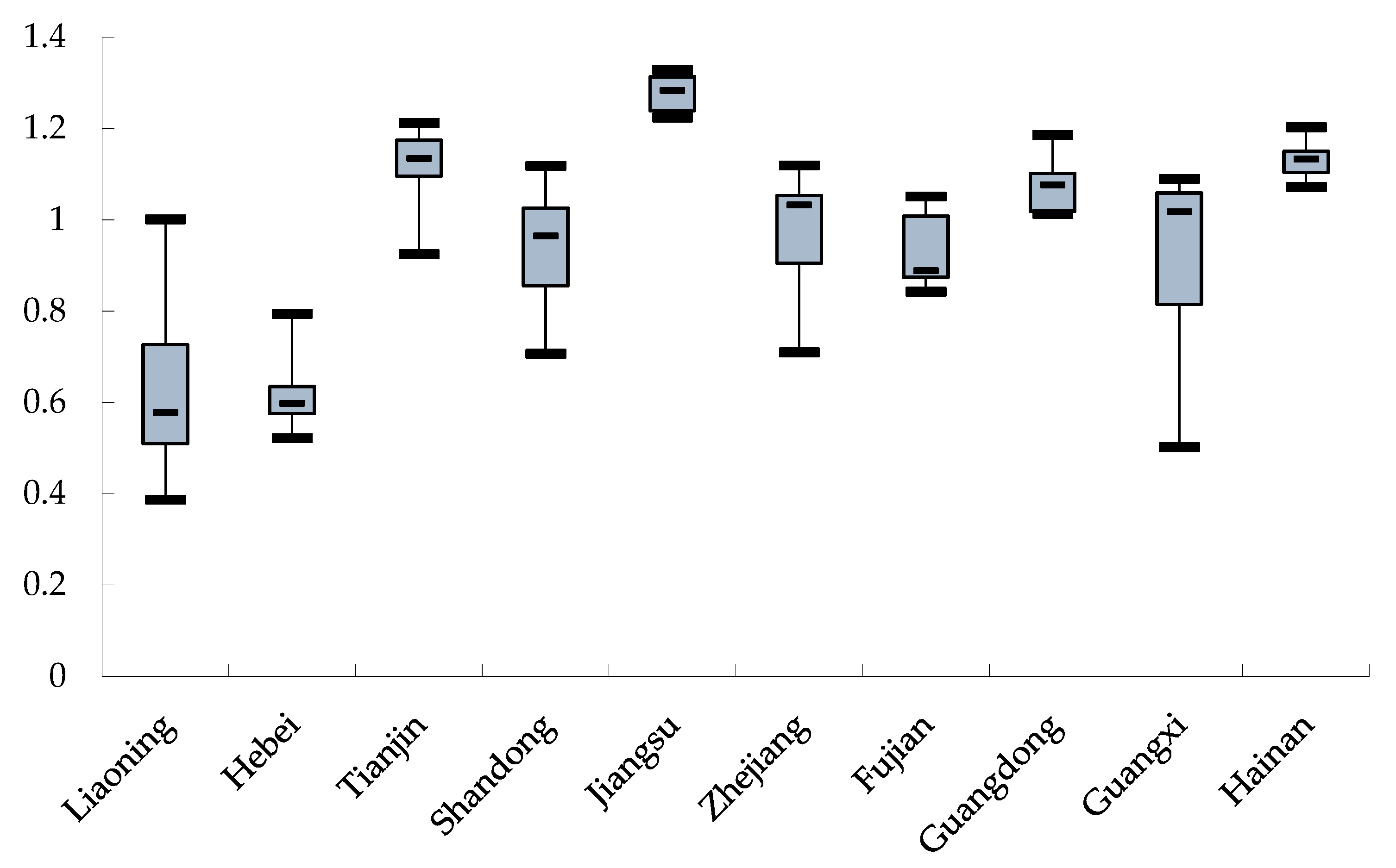
As shown the box chart of MAPE from 2008 to 2019 (Figure 2), the variance in the MAPE was very different for each province. Among these, the variances of Liaoning, Guangxi, Shandong, and Zhejiang were large, indicating that the MAPE in these regions was unstable over the 12 analyzed years and the gap between the years was significant. Guangdong, Hainan, and Jiangsu showed relatively small variances, indicating stable MAPE, and the MAPE in these regions was always at a high level, as can be seen in the box chart. Regions with relatively stable production efficiencies should maintain a good development level. Conversely, more attention should be paid to the proportion of the production input in mariculture areas and appropriate adjustments should be made.
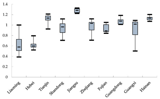
Figure 2.
Box chart of MAPE during 2008–2019.
5.1.3. Inter-Provincial Evolution Type Analysis of MAPE
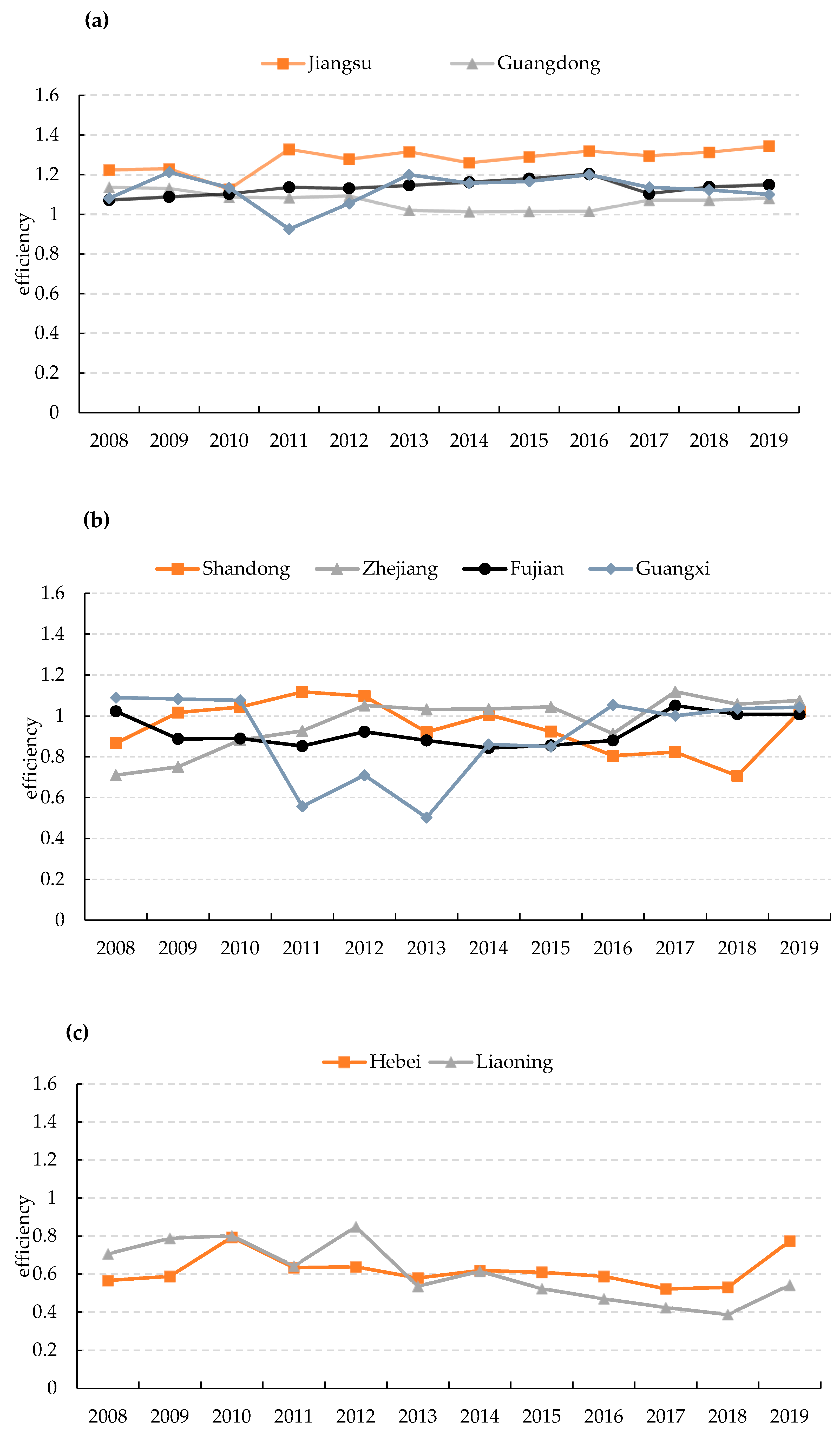
Based on the above analysis, the temporal and spatial differences in MAPE vary greatly. Referring to Sun et al. [68] and the degree of efficiency fluctuations of regions, in this study we divided the 10 coastal regions into high-efficiency stable, medium-efficiency fluctuating, and low-efficiency fluctuating types. For the high-efficiency stable type, the average MAPE is greater than 1; for the medium-efficiency fluctuating type, it fluctuates between 0.9 and 1; and for the low-efficiency fluctuating type, it is below 0.9. Therefore, the evolution characteristics of the efficiency of each province can be obtained (Figure 3).
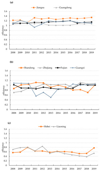
Figure 3.
Evolution types of mariculture areas’ production efficiency; (a). High-efficiency stable type; (b) Medium-efficiency fluctuating type; (c) Low-efficiency fluctuating type.
The high-efficiency stable type includes Jiangsu, Guangdong, Tianjin, and Hainan provinces (Figure 3a). Among these, the mariculture industry in Guangdong, and Jiangsu is relatively developed, the structure of their mariculture is reasonable, the scale of mariculture areas is large, and the development of mariculture is emphasized. Additionally, these four provinces are all located in the core areas of the coastal economic areas, thus being able to attract talent and create supporting facilities for mariculture. These provinces also have high levels of scientific and technological development, and the treatment of environmental pollution is more scientific, which leads to a higher production efficiency of mariculture. The main reason for the high production efficiency in Tianjin is that the exploitation of the ocean is relatively weak, and the scale of the mariculture area is relatively small, which results in less sea area pollution. Hainan has a vast sea area and abundant sea resources, and the good marine environment leads to the province requiring less input and producing more value output. Additionally, the province attaches great importance to the treatment of pollution.
The medium-efficiency fluctuating type includes Shandong, Zhejiang, Fujian, and Guangxi (Figure 3b). The MAPE of Shandong and Zhejiang was relatively low at the beginning of the study period, and the production efficiency fluctuated and increased since then, indicating that the productivity of the mariculture areas of these regions has great potential. Shandong, Fujian, and Zhejiang belong to the areas with the early development of mariculture, strong output strength, a rapidly developed economy, and a high level of scientific and technological development. However, due to the large scale of mariculture, there are more undesired outputs brought about by mariculture, which led to low efficiency in the early stage of the research. Since the implementation of the Twelfth Five-Year Guidelines of China, these areas have actively responded to the call of national policies, strengthening the construction and investment in mariculture areas, and strengthening the treatment of environmental pollution, which have greatly improved the MAPE. With the local government’s management and control of the production environment of the mariculture area, the efficiency has been improved. The main reason for the medium production efficiency in Guangxi is that economic development is relatively backward, but the local government has attached significant importance to the development of mariculture, increased inputs in mariculture, and has guaranteed sufficient financial, labor, and material resources to the development of mariculture.
The low-efficiency fluctuating type includes Hebei and Liaoning provinces (Figure 3c). In Hebei and Liaoning provinces, the foundation of mariculture is relatively poor, the method of mariculture is extensive, and the structure is unreasonable. Moreover, Hebei has a low-level economy, science, and technology, and the unreasonable treatment of undesirable outputs has resulted in a low MAPE. As the scale of mariculture expanded, the pollution caused by mariculture in Liaoning intensified. The production efficiency showed slow growth due to the pursuit of large-scale production and the neglect of undesirable outputs. Subsequently, the MAPE continued to increase in recent years based on technological innovation, policy preferences, economic advantages, and increased investment in mariculture. Sun and Ji [69] also reached a similar conclusion when they found that the factor input bias of technological progress is not satisfactory, and technological innovation and reduced dependence on resources and environment can improve the factor allocation of the mariculture industry.
5.2. Dynamic Analysis of MAPE
5.2.1. The GML and Decomposition Indexes
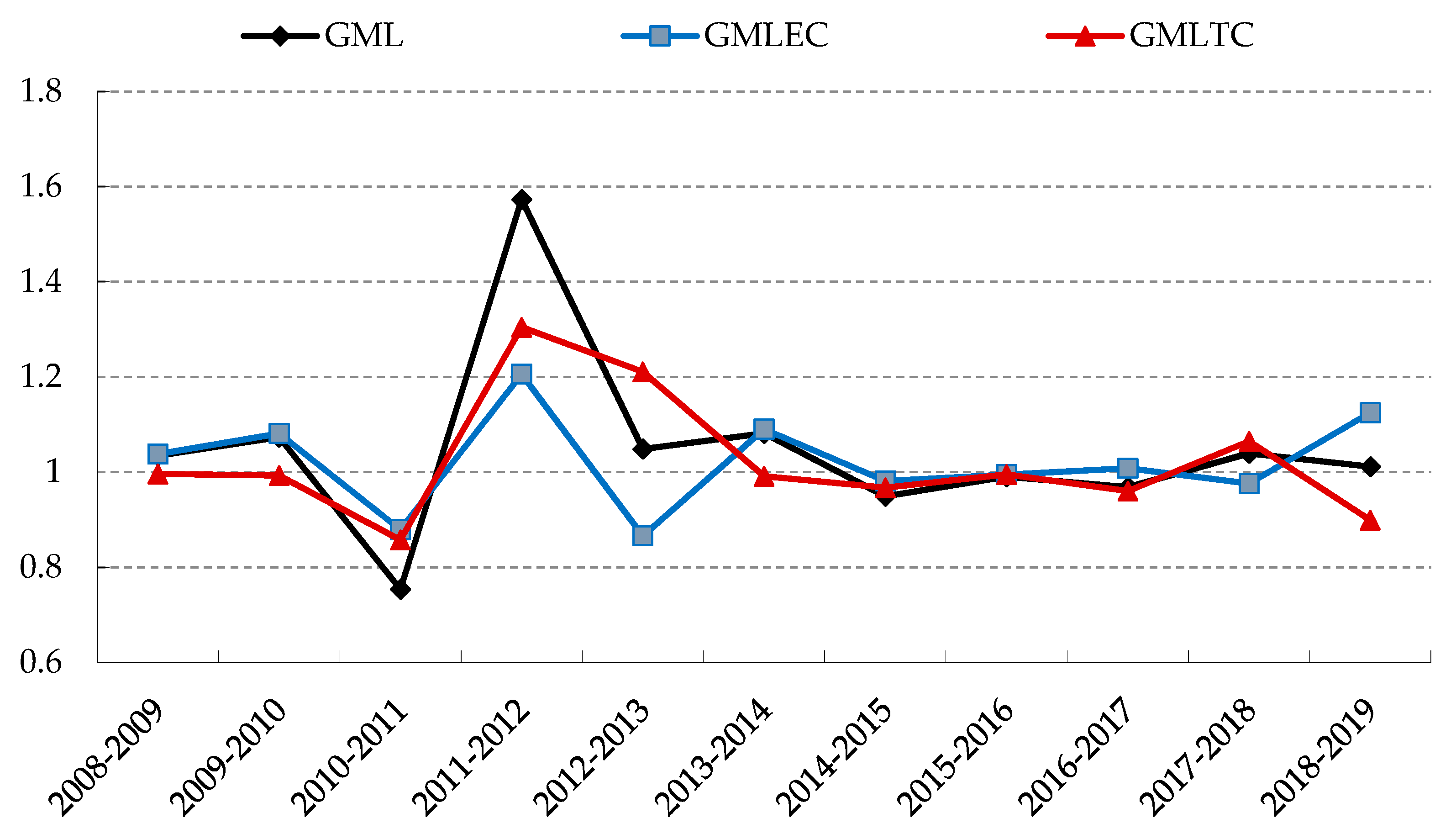
By calculating Formula (3), the GML trend of China’s mariculture areas and its decomposition index from 2008 to 2019 can be drawn (Figure 4). Based on this analysis, the GML of mariculture areas is in a state of fluctuation. The GML increased from 1.035 in 2008–2009 to 1.574 in 2011–2012, and then decreased to 0.950 in 2014–2015. Over the next four years, GML has been fluctuating. During the 12 years from 2008 to 2019, the average GML was 1.039, indicating that the production efficiency was slowly increasing. Regarding the GMLTC, from 2008 to 2019, the average change index was 1.021, indicating that the technical progress showed a fluctuating rising trend. At the same time, the change trend of the GMLTC is generally consistent with the change trend in GML, indicating that technical progress has a significant driving effect on the production efficiency. Yu et al. [27] also reached a similar conclusion when they found that the mariculture efficiency in China increased by 6.45% from 2004 to 2016, and technological progress was the main driving force for this. For the GMLEC, from 2008 to 2019, it increased from 1.038 to 1.125, and the change trend was reversed with the GML. Based on the above analysis, China attaches great importance to technological inputs and innovations in mariculture areas and constantly promotes technical progress, thus leading to an increase in the promotion of production efficiency.

Figure 4.
Temporal difference of GML and its decomposition indexes.
5.2.2. Spatiotemporal Characteristics of the GML and Decomposition Indexes
By decomposing the GML, in this study we obtained the GML and its decomposition for each province (Table 4). The GML values of nine regions were greater than one, indicating that the production efficiency was generally on the rise from 2008 to 2019 in various regions, except for Liaoning province. For the GMLEC, the efficiency indexes of Guangdong and Liaoning provinces were below one, and others were above one, showing a pattern of high technical efficiency in the center and south and of low technical efficiency in the north. All 10 regions had technical progress indexes above one, and the differences among them were small. Based on the analysis, Shandong, Liaoning, Hebei, Fujian, Guangdong, and Hainan were mainly technology-driven provinces, whereas the others showed a combination of technological progress and technological efficiency. In general, eight of the 10 mariculture areas had three indexes higher than one, and the increase in GML was mainly due to the efficiency of technical progress.
Table 4.
Spatial differences in the GML and decomposition indexes.
Four time sections were selected from 2008 to 2009, 2012 to 2013, 2015 to 2016, and 2018 to 2019 to analyze the spatiotemporal characteristics of the GML and its decomposition indexes from 2008 to 2019, considering undesirable outputs.
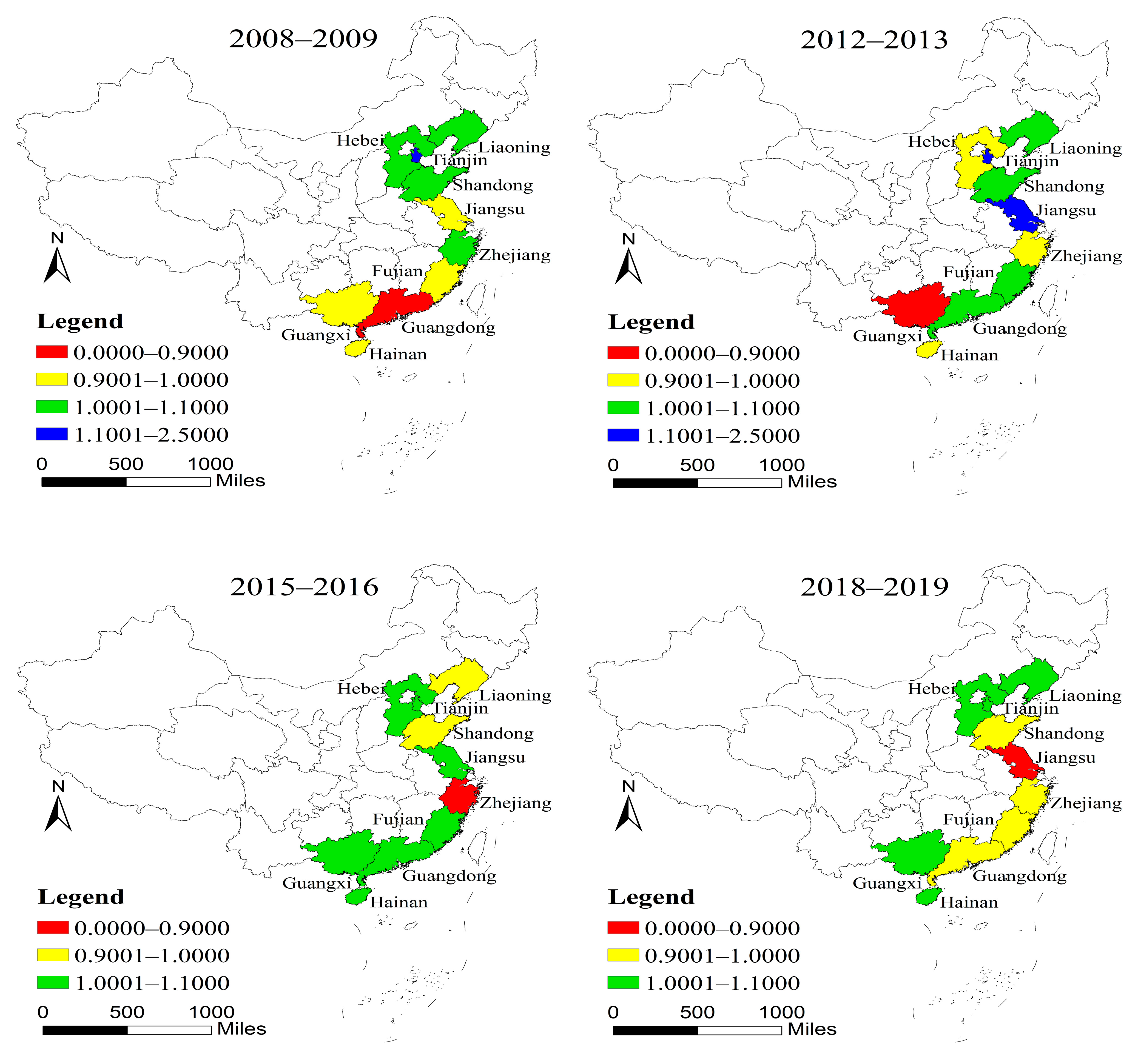
(1) The GML index (Figure 5): From 2008 to 2009, the GML values of Tianjin, Shandong, Liaoning, Hebei, and Zhejiang were greater than 1, indicating that the production efficiency of these regions increased. In other regions, the GML was less than one and the production efficiency showed a downward trend. In terms of space and geography, production efficiency showed an upward trend in the north and central region and a downward trend in the south. From 2012 to 2013, the GML values of Hainan, Guangxi, Hebei, and Zhejiang were less than one, indicating that the production efficiency showed a downward trend. From 2015 to 2016, all values, except for the production efficiency in Liaoning, Shandong and Zhejiang, showed a downward trend, whereas the other regions showed an upward trend, with slight increases. From 2018 to 2019, the production efficiency in Jiangsu, Shandong, Guangdong, Fujian, and Zhejiang showed a downward trend, whereas the rest showed a slight increase; in general, the north and south regions showed an upward trend.

Figure 5.
Spatial changes in GML of production efficiency.
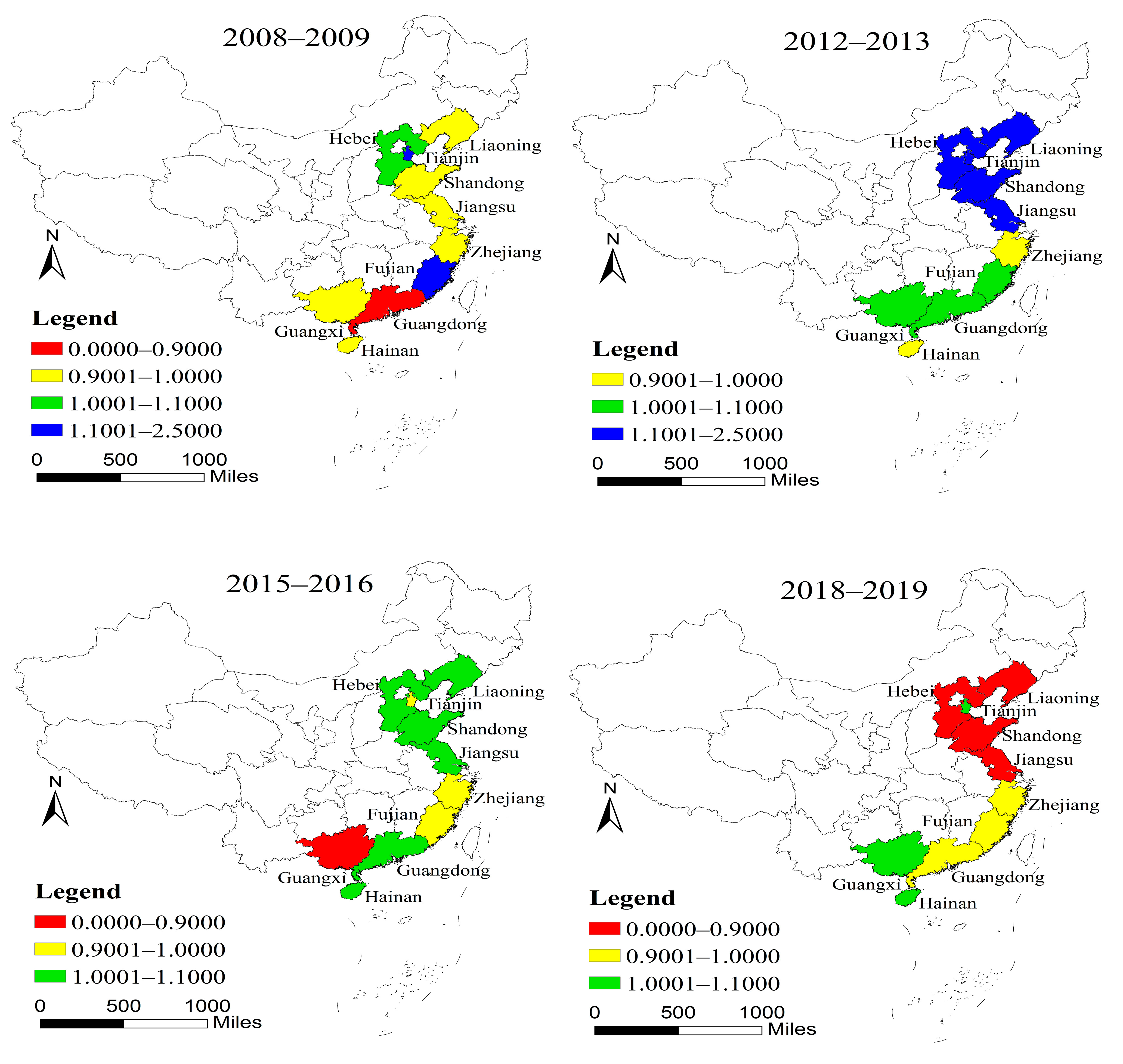
(2) The GMLTC index (Figure 6): From 2008 to 2009, the change index of GMLTC in Tianjin, Hebei, and Fujian was greater than one, showing an upward trend. The other regions showed different degrees of decline. Namely, the spatial pattern of the technological progress showed an upward trend in the central and north region and a downward trend in the south. There was a major change from 2012 to 2013, with the exception of Hainan and Zhejiang, which showed a slow downward trend, whereas the other regions experienced a sharp increase. In terms of space and geography, there was a downward trend in the south and central region and an upward trend in the north. Except for Guangxi, Tianjin, Fujian, and Zhejiang, the GMLTC of which remained less than one from 2015 to 2016, all other regions showed an upward trend, and the increase was relatively small. During 2018–2019, the GMLTC index of Liaoning, Hebei, Shandong, and Jiangsu decreased significantly, and only the indexes of Guangxi, Hainan, and Tianjin were greater than one, indicating that the technological progress of these three regions had increased. On the whole, the GMLTC index showed a trend of increasing first and then decreasing, and the changes in the south and north regions were more obvious, and the changes in the middle were smaller.

Figure 6.
Spatial changes in GMLTC.
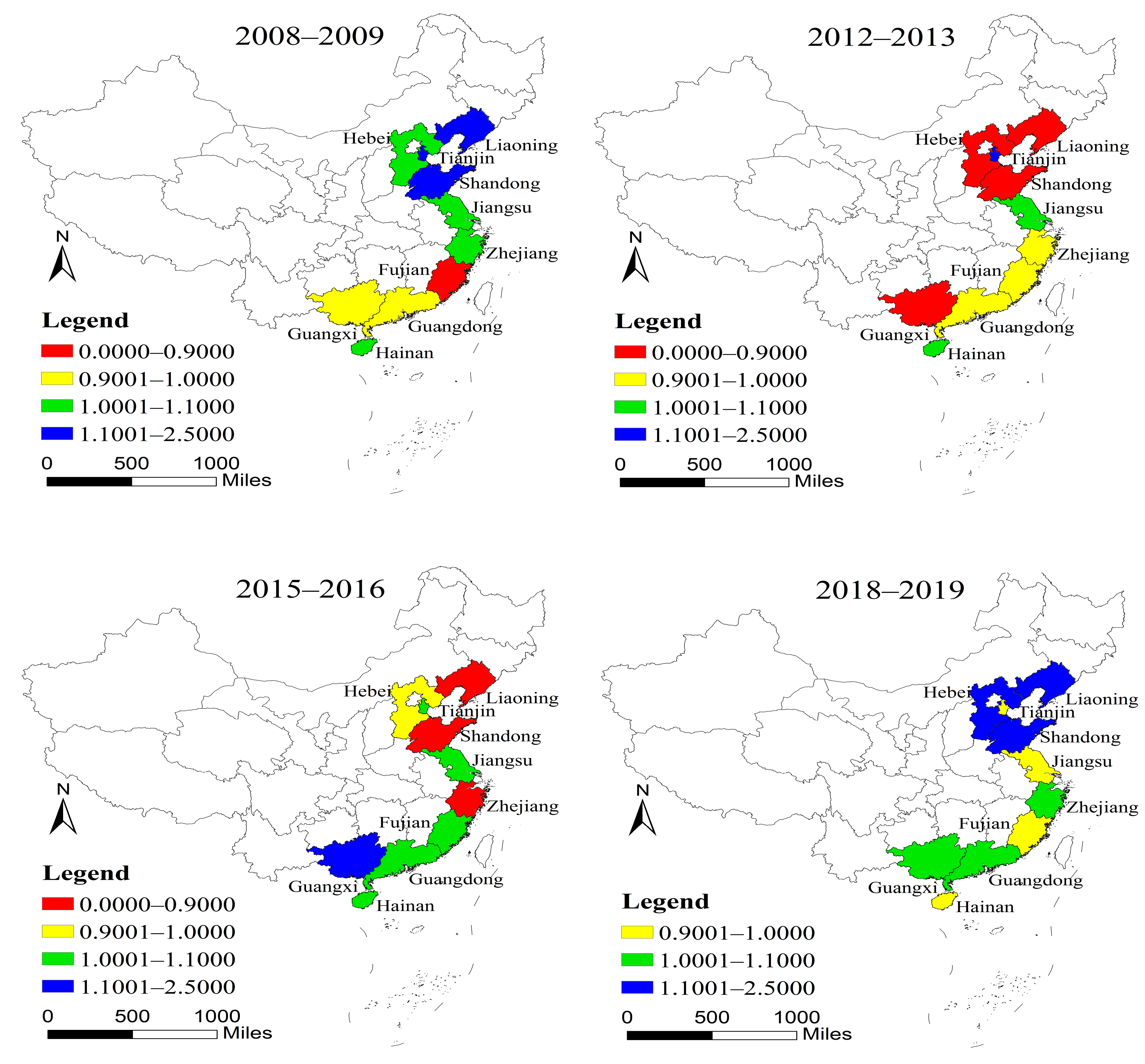
(3) GMLEC index (Figure 7): From 2008 to 2009, in addition to Guangxi, Guangdong, and Fujian, the GMLEC index of other regions was greater than one, indicating that technical efficiency showed an upward trend. The indexes of Hebei, Jiangsu, Zhejiang, and Hainan were close to one, indicating that there was no significant change in technical efficiency during the research phase. From 2012 to 2013, Liaoning, Hebei, Shandong, and Guangxi showed a significant downward trend, whereas the other regions showed little change. From 2015 to 2016, only the GMLEC of Liaoning, Shandong, Hebei, and Zhejaing showed a downward trend, whereas the indexes of other regions showed an upward trend. From 2018 to 2019, Liaoning, Hebei, and Shandong showed a significant upward trend, whereas Tianjin, Jiangsu, Fujian, and Hainan showed a slow downward trend. Overall, technical efficiency showed a trend of first decreasing and then increasing, and the change in the technical efficiency index in the northern region was more obvious.
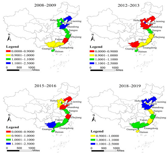
Figure 7.
Spatial changes in GMLEC.
5.3. Spatial Difference Decomposition of MAPE
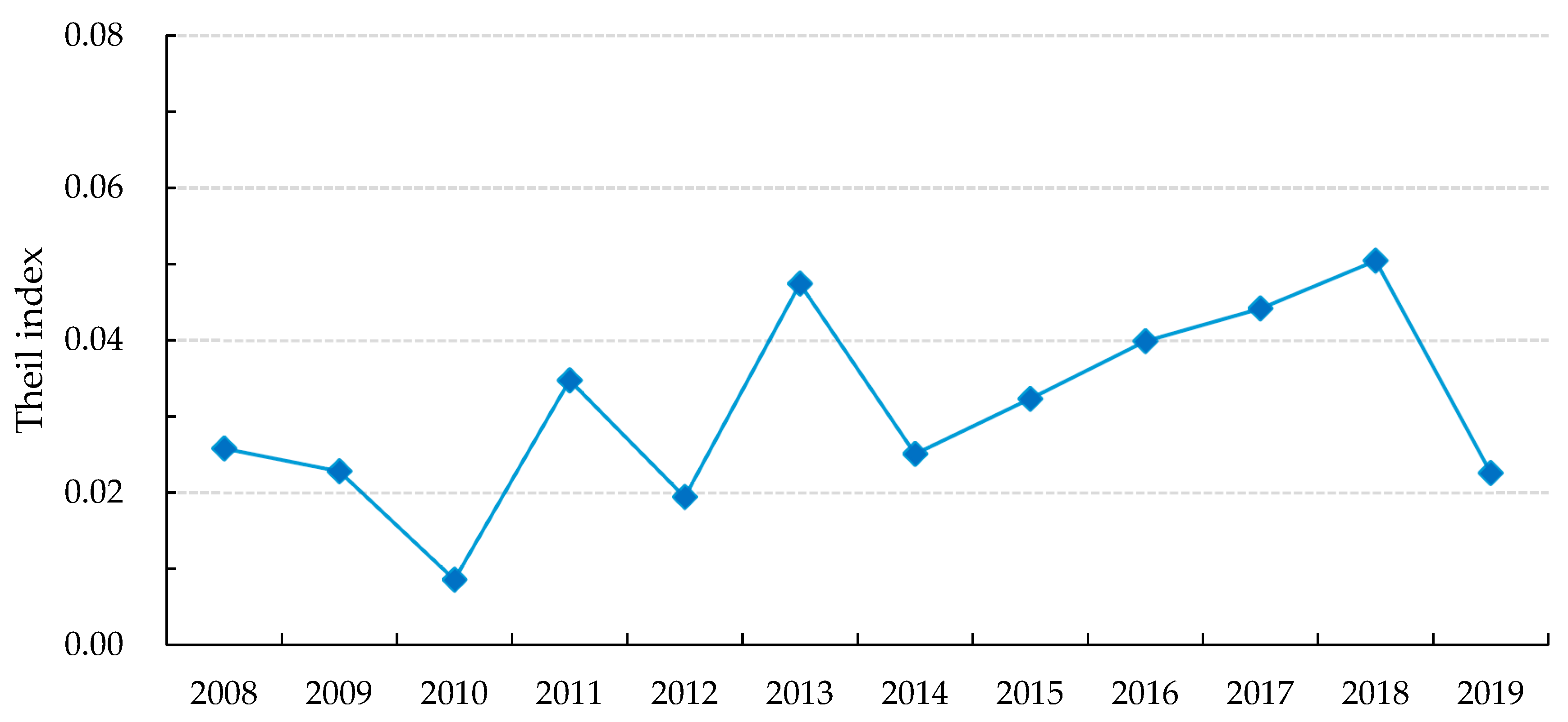
Based on the above analysis, there were significant spatiotemporal disparities in terms of MAPE in China’s east coast from both static and dynamic perspectives. To explore the structure and causes of the differences in production efficiency among regions, in this study we used the Theil index to decompose the differences in MAPE [70], as per Figure 8. Overall, the MAPE in the coastal regions differed significantly from 2008 to 2019, and the Theil index fell rapidly from 0.026 in 2008 and 0.023 in 2009 to 0.009 in 2010, and the difference between regions reached the lowest value. Since then, it tortuously increased to 0.005 in 2018. The overall trend is represented by a decline, followed by an increase, and then a decrease, indicating that the differences in MAPE first decreased and then increased, and finally decreased. To further explore the causes of the differences and to narrow them in MAPE, in this study we analyzes these structural differences and condense the 10 regions into three regions based on existing research [71]. Among them, the circum-Bohai Sea region includes the Liaoning, Hebei, Tianjin, and Shandong provinces; the Yangtze River Delta region includes the Jiangsu, Zhejiang, and Fujian provinces; and the Pearl River Delta region includes the Guangdong, Guangxi, and Hainan provinces.
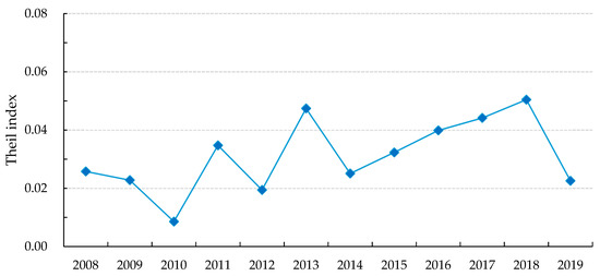
Figure 8.
Theil indexes of MAPE from 2008 to 2019.
By calculating Formulas (8) and (9), the decomposition results of the Theil index for the regional groups can be obtained (Table 5). From 2008 to 2019, the relationship between the intra- and inter-regional difference contribution rates of MAPE changed significantly. The intra-regional difference contribution rate increased from 66.37% to 87.67% and then decreased to 64.06%, whereas the inter-regional difference contribution rate decreased from 33.63% to 12.33% and then increased to 35.92%, which means that the role of the intra-regional differential contribution rate first strengthened and then weakened, and the inter-regional difference contribution rate first weakened and then strengthened. From 2009 to 2014, the contribution rate of intra-regional differences exceeded 80.00%, indicating that intra-regional differences occupied an absolute dominant position in the overall differences. Although it was still dominated by intra-regional differences, the situation changed significantly in 2018, with the contribution rate falling to 50.59%. Then, in 2019, the contribution rate of intra-regional differences increased. Overall, intra-regional differences were always the dominant factor for MAPE differences. This is similar to the results of agricultural studies. Pang et al. [72] examined the regional differences and spatiotemporal patterns of the carbon emission intensity of agriculture production, and the results showed that the overall differences were caused by intra-regional differences.
Table 5.
Contribution rate of the Theil index decomposition from 2008 to 2019.
At the same time, the main factors causing intra-regional differences also changed. The intra-regional differences in the circum-Bohai Sea region showed an upward trend, whereas the Pearl River Delta region was in a relatively stable state of development but showing a downward trend, with the greatest degree of decline being from 28.73% at the beginning of the study period to 11.74% at the end of the study period. In general, from 2008 to 2019, the intra-regional differences in the circum-Bohai Sea region were the main reason for the overall intra-regional differences, whereas the Yangtze River Delta was the secondary factor. However in 2011, the intra-regional differences in the Yangtze River Delta region became the main factor influencing the overall intra-regional differences, followed by the circum-Bohai Sea region and the Pearl River Delta region. Analyzing the Theil index of MAPE, we note that intra-regional differences are the main factor causing the differences in MAPE, but the contribution of the inter-regional differences to the overall difference is increasing.
6. Conclusions and Discussion
6.1. Main Conclusions and Policy Implications
This study analyzed the spatiotemporal disparities of MAPE from both static and dynamic perspectives. Using the S-EBM model and considering undesirable outputs, the MAPE of 10 coastal regions in China as the measurement object was measured and analyzed statically from 2008 to 2019. The GML index was further used to dynamically depict the production efficiency, and the Theil index was used to analyze the main reasons for the spatial differences in MAPE. The main conclusions are as follows.
Based on the static analysis, the MAPE showed fluctuations and increased from 2008 to 2019, and the overall level of MAPE was relatively high, namely, in the medium-high efficiency area. The efficiency of each province differed greatly and the overall spatial pattern was high in the center and south and low in the north. Based on the analysis of the spatiotemporal differentiation, the efficiency evolution can be divided into three types: high-efficiency stable, medium-efficiency fluctuating, and low-efficiency fluctuating.
Based on the dynamic analysis, regarding the GML and GMLTC, the production efficiency and technical progress showed a fluctuating rising trend, and technical progress had a significant driving effect on the production efficiency. The GML of production efficiency in the north and south region showed an upward trend, the GMLTC in the south and north regions were more obvious, and the changes in the middle were smaller, and the GMLEC in the northern region was more obvious.
Based on the Theil index and its contribution rate, the differences in MAPE first decreased and then increased, and finally decreased. The role of the intra-regional differential contribution rate first strengthened and then weakened, and the inter-regional first weakened and then strengthened. Intra-regional differences were the main factors that caused the differences in MAPE and the intra-regional differences in the circum-Bohai Sea region were the main reason for the overall intra-regional differences.
Based on these results, there are several policy implications for improving the MAPE in China. First, attention should be paid to the balanced development of each region, and regions with low production efficiency should further increase scientific and technological investment in mariculture, and seek more reasonable mariculture methods; second, the government should establish a monitoring center for the pollution of mariculture areas to strengthen supervision and guidance; furthermore, policies for exchange and cooperation among different mariculture areas need to be introduced to promote information sharing and technical exchange, to narrow regional differences in MAPE, and to achieve sustainable development.
6.2. Limitations and Discussions
These empirical results are of great significance for understanding how to strengthen the sustainable development and utilization of mariculture areas from the perspective of production efficiency. Reducing undesirable output and narrowing regional differences are the preferred strategies to improve the MAPE. This can be reflected indirectly through measurement of the input-output indicators of MAPE and the further analysis of the spatiotemporal disparities. Beyond that, there should be some limitations and discussion about our proposed models and findings that provide useful directions for the future research. A limitation of this study was that it ignored more possible relevant factors other than the region, such as mariculture structure and mariculture mode. The regression analysis with the efficiency score as the dependent variable should comprehensively consider the impact of other influencing factors on the MAPE. In addition, an environmental control group should be added, and the expected and unexpected data should be compared and analyzed in future research. Furthermore, in our study we took 10 coastal regions as samples, with a small number and a relatively broad range. We are considering extending the sample to coastal prefecture-level cities in the future, and the research results may be more representative. Of course, if the data are available, coastal regions of other countries will also be an object of our study. Such research is more intuitive and interesting and can provide help for the sustainable development of mariculture areas.
Author Contributions
Conceptualization, J.J. and Y.X.; methodology, L.L.; software, L.L. and N.Z.; validation, L.L. and N.Z.; formal analysis, J.J. and Y.X.; visualization, Y.X.; resources, J.J.; data curation, L.L., Y.X., and N.Z.; writing—review and editing, L.L. and Y.X. All authors have read and agreed to the published version of the manuscript.
Funding
This work was supported by the National Natural Science Foundation of China (Grant No.71873127, Grant No.71573238), National Social Science Found of China (Grant No.19VHQ007), and Major Project of Social Science Planning of Shandong Province (Grant No. 20AWTJ19).
Institutional Review Board Statement
Not applicable.
Informed Consent Statement
Not applicable.
Data Availability Statement
The data for this study are available through the corresponding author.
Acknowledgments
The authors thank the editor and the anonymous reviewers for providing constructive suggestions and comments on the manuscript.
Conflicts of Interest
The authors report no declarations of interest.
Abbreviations
| COD | Chemical oxygen demand |
| DEA | Data envelope analysis |
| DMU | Decision-making unit |
| EBM | Engel–Blackwell–Miniard |
| GML | Global Malmquist–Luenberger |
| GMLEC | Global Malmquist–Luenberger technical efficiency |
| GMLTC | Global Malmquist–Luenberger technical progress |
| LCA | Life cycle assessment |
| MAPE | Mariculture area production efficiency |
| N | Nitrogen |
| P | Phosphorus |
| SBM | Slacks-based measure |
| S-EBM | Super-efficiency Engel–Blackwell–Miniard |
| SFA | Stochastic frontier analysis |
| TFP | Total factor productivity |
| TTP | Tornqvists–Theil |
References
- Skallerud, K.; Armbrecht, J. A segmentation of residents’ attitudes towards mariculture development in Sweden. Aquaculture 2020, 521, 735040. [Google Scholar] [CrossRef]
- Yu, J.K.; Han, Q.C. Food security of mariculture in China: Evolution, future potential and policy. Mar. Pol. 2020, 115, 103892. [Google Scholar] [CrossRef]
- Food and Agriculture Organization of the United Nations (FAO). The State of World Fisheries and Aquaculture (2020); FAO Fisheries and Aquaculture Department: Rome, Italy, 2020. [Google Scholar]
- Costello, C.; Cao, L.; Gelcich, S.; Cisneros-Mata, M.Á.; Free, C.M.; Froehlich, H.E.; Golden, C.D.; Ishimura, G.; Maier, J.; Macadam-Somer, I.; et al. The future of food from the sea. Nature 2020, 588, 95–100. [Google Scholar] [CrossRef] [PubMed]
- Campbell, B.; Pauly, D. Mariculture: A global analysis of production trends since 1950. Mar. Pol. 2013, 39, 94–100. [Google Scholar] [CrossRef]
- Yu, J.K.; Yin, W.; Liu, D.H. Evolution of mariculture policies in China: Experience and challenge. Mar. Pol. 2020, 119. [Google Scholar] [CrossRef]
- Fisheries Administration of Ministry of Agriculture and Rural Affairs of the People’ s Republic of China (FAPRC). China Fisheries Yearbook. China Agricultural Press, Beijing, 2014–2019. Available online: https://www.cafs.ac.cn/info/1397/31337.htm (accessed on 23 November 2021).
- Ministry of Agriculture and Rural Affairs, Ministry of Ecology and Environment. Report on the state of the fishery eco-environment in China. 2018. Available online: https://www.cafs.ac.cn/kxyj/sjfw/yysthjzkgb.htm (accessed on 23 November 2021).
- Ding, L.L.; Lei, L.; Wang, L.; Zhang, L.F.; Calin, A.C. A novel cooperative game network DEA model for marine circular economy performance evaluation of China. J. Clean. Prod. 2020, 253, 120071. [Google Scholar] [CrossRef]
- Ren, W.H.; Ji, J.Y.; Chen, L.; Zhang, Y. Evaluation of China’ s marine economic efficiency under environmental constraints: An empirical analysis of China’ s eleven coastal regions. J. Clean. Prod. 2018, 184, 806–814. [Google Scholar] [CrossRef]
- Xia, K.; Guo, J.K.; Han, Z.L.; Dong, M.R.; Xu, Y. Analysis of the scientific and technological innovation efficiency and regional differences of the land–sea coordination in China’ s coastal areas. Ocean Coast Manag. 2019, 172, 157–165. [Google Scholar] [CrossRef]
- Yin, K.D.; Xu, Y.; Li, X.M.; Jin, X. Sectoral relationship analysis on China’ s marine-land economy based on a novel grey periodic relational model. J. Clean. Prod. 2018, 197, 815–826. [Google Scholar] [CrossRef]
- Ren, W.H.; Ji, J.Y. How do environmental regulation and technological innovation affect the sustainable development of marine economy: New evidence from China’ s coastal provinces and cities. Mar. Pol. 2021, 128, 104468. [Google Scholar] [CrossRef]
- Pan, Z.; Tan, Y.M.; Gao, W.F.; Dong, S.L.; Fang, X.D.; Yan, J.L. A 120-year record of burial fluxes and source apportionment of sedimentary organic carbon in Alian Bay, China: Implication for the influence of mariculture activities, and regional environment changes. Aquaculture 2021, 535, 736421. [Google Scholar] [CrossRef]
- Sun, K.; Zhang, J.H.; Lin, F.; Ren, J.S.; Zhao, Y.X.; Wu, W.G.; Liu, Y. Evaluating the growth potential of a typical bivalve-seaweed integrated mariculture system: A numerical study of Sungo Bay, China. Aquaculture 2021, 532, 736037. [Google Scholar] [CrossRef]
- Xu, Y.; Ji, J.Y.; Xu, Y.J. Spatial disequilibrium of mariculture areas utilization efficiency in China and causes. Resour. Sci. 2020, 42, 2158–2169. [Google Scholar] [CrossRef]
- Fukase, E.; Martin, W. Who will feed China in the 21st century? Income growth and food demand and supply in China. J. Agric. Econ. 2015, 67, 3–23. [Google Scholar] [CrossRef]
- Han, L.M.; Li, D.H. Blue food system: Guarantee of China’ s food security. Issues Agric. Econ. 2015, 36, 24–29+110. [Google Scholar]
- Li, D.; Nanseki, T.; Takeuchi, S. Measurement of agricultural production efficiency and the determinants in China based on a DEA approach: A case study of 99 farms from Hebei province. J. Fac. Agric. Kyushu Univ. 2012, 57, 235–244. [Google Scholar] [CrossRef]
- Yang, C.H.; Wu, L.; Lin, H.L. Analysis of total-factor cultivated land efficiency in China’ s agriculture. Agric. Econ. 2010, 56, 231–242. [Google Scholar]
- Zhu, X.; Zhang, P.; Wei, Y.; Li, Y.; Zhao, H. Measuring the efficiency and driving factors of urban land use based on the DEA method and the PLS-SEM model: A case study of 35 large and medium-sized cities in China. Sustain. Cities Soc. 2019, 50, 101646. [Google Scholar] [CrossRef]
- Wang, S.H.; Lu, B.B.; Yin, K.D. Financial development, productivity, and high-quality development of the marine economy. Mar. Pol. 2021, 130, 104553. [Google Scholar] [CrossRef]
- Wang, Y.X.; Wang, N. The role of the marine industry in China’ s national economy: An input–output analysis. Mar. Pol. 2019, 99, 42–49. [Google Scholar] [CrossRef]
- Wang, X.H. A study on ecological efficiency measurement and promoting countermeasures of marine utilization: A case of Zhejiang province. East China Econ. Manag. 2018, 32, 22–29. [Google Scholar]
- Ji, J.Y.; Guo, X.; Zhang, Y. The study of symbiotic relationships between the economic and the ecological system of China’ s mariculture industry: An empirical analysis of 10 coastal regions with Lokta–Volterra model. Reg. Stud. Mar. Sci. 2021, 48, 102051. [Google Scholar] [CrossRef]
- Salayo, N.D.; Perez, M.L.; Garces, L.R.; Pido, M.D. Mariculture development and livelihood diversification in the Philippines. Mar. Pol. 2012, 36, 867–881. [Google Scholar] [CrossRef]
- Yu, X.; Hu, Q.; Shen, M. Provincial differences and dynamic changes in mariculture efficiency in China: Based on Super-SBM model and global Malmquist index. Biology 2020, 9, 18. [Google Scholar] [CrossRef] [Green Version]
- Polthanee, A.; Trelo-ges, V. Growth, yield and land use efficiency of corn and legumes grown under intercropping systems. Plant Prod. Sci. 2003, 6, 139–146. [Google Scholar] [CrossRef]
- Seufert, V.; Ramankutty, N.; Foley, J.A. Comparing the yields of organic and conventional agriculture. Nature 2012, 485, 229–232. [Google Scholar] [CrossRef] [PubMed]
- Zhao, Z.B.; Shi, X.P.; Zhao, L.D.; Zhang, J.G. Extending production-theoretical decomposition analysis to environmentally sensitive growth: Case study of Belt and Road Initiative countries. Technol. Forecast. Soc. Chang. 2020, 161, 120289. [Google Scholar] [CrossRef]
- Wang, L.J.; Li, H. Cultivated land use efficiency and the regional characteristics of its influencing factors in China: By using a panel data of 281 prefectural cities and the stochastic frontier production function. Geogr. Res. 2014, 33, 1995–2004. [Google Scholar]
- Wang, S.H.; Yu, H.; Song, M.L. Assessing the efficiency of environmental regulations of large-scale enterprises based on extended fuzzy data envelopment analysis. Ind. Manag. Data Syst. 2018, 118, 463–479. [Google Scholar] [CrossRef]
- Zhao, Z.B.; Yuan, T.; Shi, X.P.; Zhao, L.D. Heterogeneity in the relationship between carbon emission performance and urbanization: Evidence from China. Mitig. Adapt. Strateg. Glob. Chang. 2020, 25, 1363–1380. [Google Scholar] [CrossRef]
- Ding, L.L.; Yang, Y.; Wang, L.; Calin, A.C. Cross Efficiency assessment of China’ s marine economy under environmental governance. Ocean Coast Manag. 2020, 193, 105245. [Google Scholar] [CrossRef]
- Charnes, A.; Cooper, W.W.; Rhodes, E. Measuring the efficiency of decision making units. Eur. J. Oper. Res. 1978, 2, 429–444. [Google Scholar] [CrossRef]
- Jradi, S.; Ruggiero, J. Stochastic data envelopment analysis: A quantile regression approach to estimate the production frontier. Eur. J. Oper. Res. 2019, 278, 385–393. [Google Scholar] [CrossRef]
- Shabanzadeh-Khoshrody, M.; Azadi, H.; Khajooeipour, A.; Nabavi-Pelesaraei, A. Analytical investigation of the effects of dam construction on the productivity and efficiency of farmers. J. Clean. Prod. 2016, 135, 549–557. [Google Scholar] [CrossRef]
- Van Nguyen, Q.; Pascoe, S.; Coglan, L.; Nghiem, S. The sensitivity of efficiency scores to input and other choices in stochastic frontier analysis: An empirical investigation. J. Prod. Anal. 2021, 55, 31–40. [Google Scholar] [CrossRef]
- Wang, Y.Z.; Li, X.; Xu, Q.; Ying, L.M.; Lai, C.H.; Li, A. Evaluation of soil and water conservation performance under promotion incentive based on stochastic frontier function model. Alex. Eng. J. 2022, 61, 855–862. [Google Scholar] [CrossRef]
- Wang, S.H.; Lei, L.; Xing, L. Urban circular economy performance evaluation: A novel fully fuzzy data envelopment analysis with large datasets. J. Clean. Prod. 2021, 324, 129214. [Google Scholar] [CrossRef]
- Han, H.B.; Zhang, X.Y. Static and dynamic cultivated land use efficiency in China: A minimum distance to strong efficient frontier approach. J. Clean. Prod. 2020, 246, 119002. [Google Scholar] [CrossRef]
- Li, Q.F.; Hu, S.G.; Du, G.M.; Zhang, C.R.; Liu, Y.S. Cultivated land use benefits under state and collective agrarian property regimes in China. Sustainability 2018, 10, 7. [Google Scholar] [CrossRef] [Green Version]
- Lu, X.H.; Kuang, B.; Li, J.; Han, J.; Zhang, Z. Dynamic evolution of regional discrepancies in carbon emissions from agricultural land utilization: Evidence from Chinese provincial data. Sustainability 2018, 10, 552. [Google Scholar] [CrossRef] [Green Version]
- Guo, J.H.; Liu, X.J.; Zhang, Y.; Shen, J.L.; Han, W.X.; Zhang, W.F.; Christie, P.; Goulding, K.W.T.; Vitousek, P.M.; Zhang, F.S. Significant acidification in major Chinese croplands. Science 2020, 327, 1008–1010. [Google Scholar] [CrossRef] [Green Version]
- Wang, S.H.; Sun, X.L.; Song, M.L. Environmental regulation, resource misallocation, and ecological efficiency. Emerg. Mark. Financ. Trade 2021, 57, 410–429. [Google Scholar] [CrossRef]
- Zhang, H.; Wang, B.; Xu, M.; Fan, T. Crop yield and soil responses to long-term fertilization on a red soil in southern China. Pedosphere 2019, 19, 199–207. [Google Scholar] [CrossRef]
- Wang, S.H.; Zhao, D.Q.; Chen, H.X. Government corruption, resource misallocation, and ecological efficiency. Energy Econ. 2020, 85, 104573. [Google Scholar] [CrossRef]
- Saber, Z.; Zelm, R.; Pirdashti, H.; Schipper, A.M.; Esmaeili, M.; Motevali, A.; Nabavi-Pelesaraei, A.; Huijbregts, M.A.J. Understanding farm-level differences in environmental impact and eco-efficiency: The case of rice production in Iran. Sustain. Prod. Consump. 2021, 27, 1021–1029. [Google Scholar] [CrossRef]
- Nabavi-Pelesaraei, A.; Azadi, H.; Passel, S.V.; Saber, Z.; Hosseini-Fashami, F.; Mostashari-Rad, F.; Ghasemi-Mobtaker, H. Prospects of solar systems in production chain of sunflower oil using cold press method with concentrating energy and life cycle assessment. Energy 2021, 223, 120117. [Google Scholar] [CrossRef]
- Singh, K. Farm specific economic efficiency of fish production in south tripura district: A stochastic frontrier approach. Indian J. Agric. Econ. 2008, 63, 598–613. [Google Scholar]
- Nielsen, R. Green and technical efficient growth in Danish fresh water aquaculture. Aquac. Econ. Manag. 2011, 15, 262–277. [Google Scholar] [CrossRef]
- Ji, J.Y.; Wang, P.P. Research on China’ s aquaculture efficiency evaluation and influencing factors with undesirable outputs. J. Ocean Univ. China 2015, 14, 569–574. [Google Scholar] [CrossRef]
- Wang, P.P.; Ji, J.Y. Research on China’ s mariculture efficiency evaluation and influencing factors with undesirable outputs: An empirical analysis of China’ s ten coastal regions. Aquac. Int. 2017, 25, 1521–1530. [Google Scholar] [CrossRef]
- Vassdal, T.; Holst, H.M.S. Technological progress and regress in Norwegian Salmon farming: A malmquist index approach. Mar. Resour. Econ. 2011, 26, 329–341. [Google Scholar] [CrossRef]
- Ji, J.Y.; Sun, Q.W.; Ren, W.H.; Wang, P.P. The Spatial spillover effect of technical efficiency and its influencing factors for China’ s mariculture: Based on the partial differential decomposition of a spatial durbin model in the coastal provinces. Iran. J. Fish. Sci. 2020, 19, 921–933. [Google Scholar]
- Zhao, L.; Zhang, Y.S.; Wu, D. Marine economic efficiency and spatio-temporal characteristics of inter-province based on undesirable output in China. Sci. Geogr. 2016, 36, 32–41. [Google Scholar]
- Tone, K. A slacks-based measure of efficiency in data envelopment analysis. Eur. J. Oper. Res. 2001, 130, 498–509. [Google Scholar] [CrossRef] [Green Version]
- Tone, K.; Tsutsui, M. An epsilon-based measure of efficiency in DEA-a third pole of technology efficiency. Eur. J. Oper. Res. 2010, 207, 1554–1563. [Google Scholar] [CrossRef]
- Andersen, P.; Petersen, N.C. A procedure for ranking efficientunits in data envelopment analysis. Manag. Sci. 1993, 39, 1261–1264. [Google Scholar] [CrossRef]
- Li, M.; Wang, J. Spatial-temporal distribution characteristics and driving mechanism of green total factor productivity in China’ s logistics industry. Pol. J. Environ. Stud. 2021, 30, 201–213. [Google Scholar] [CrossRef]
- Oh, D.H. A global Malmquist-Luenberger productivity index. J. Prod. Anal. 2010, 34, 183–197. [Google Scholar] [CrossRef]
- Chung, Y.H.; Fare, R.; Grosskopf, S. Productivity and undesirable outputs: A directional distance function approach. J. Environ. Manag. 1997, 51, 229–240. [Google Scholar] [CrossRef] [Green Version]
- Liu, H.W.; Yang, R.L.; Wu, D.D.; Zhou, Z.X. Green productivity growth and competition analysis of road transportation at the provincial level employing Global Malmquist-Luenberger Index approach. J. Clean. Prod. 2021, 279, 123677. [Google Scholar] [CrossRef]
- Yang, Q.; Liu, H.J. Regional difference decomposition and influence factors of China’ s carbon dioxide emissions. J. Quant. Tech. 2012, 29, 36–49+148. [Google Scholar]
- Fan, S.G.; Zhang, X.B.; Sherman, R. Structural change and economic growth in China. China Econ. Q. 2002, 4, 181–198. [Google Scholar] [CrossRef]
- Ji, J.Y.; Li, Y.F. Research on green technology progress measurement and influencing factors in marine aquaculture industry in China. J. Ocean Univ. (Soc. Sci.) 2019, 4, 45–50. [Google Scholar]
- Tu, Z.G. The coordination of industrial growth with environment and resource. Econ. Res. J. 2008, 4, 93–105. [Google Scholar]
- Sun, K.; Ji, J.W.; Li, L.D.; Zhang, C.; Liu, J.F.; Fu, M. Marine fishery economic efficiency and its spatiotemporal differences based on undesirable outputs in China. Resour. Sci. 2017, 39, 2040–2051. [Google Scholar]
- Sun, Y.N.; Ji, J.Y. Measurement and analysis of technological progress bias in China’ s mariculture industry. J. World Aquacult. Soc. 2021, 1–17. [Google Scholar] [CrossRef]
- Gai, Z.X.; Sun, P.; Zhang, J.Q. Cultivated land utilization efficiency and its difference with consideration of environmental constraints in major grain producing area. Econ. Geogr. 2017, 37, 163–171. [Google Scholar]
- Liu, J.; Lu, J.; Liu, N. Space-time evolution, influencing factors and forming mechanisms of tourism industry’ s efficiency in China’ s coastal area of based on DEA-Malmquist model. Resour. Sci. 2015, 37, 2381–2393. [Google Scholar]
- Pang, J.X.; Li, H.J.; Lu, C.P.; Lu, C.Y.; Chen, X.P. Regional differences and dynamic evolution of carbon emission intensity of agriculture production in China. Int. J. Environ. Res. Public Health 2020, 17, 7541. [Google Scholar] [CrossRef]
Publisher’s Note: MDPI stays neutral with regard to jurisdictional claims in published maps and institutional affiliations. |
© 2022 by the authors. Licensee MDPI, Basel, Switzerland. This article is an open access article distributed under the terms and conditions of the Creative Commons Attribution (CC BY) license (https://creativecommons.org/licenses/by/4.0/).