Evaluating the Effects of the Rill Longitudinal Profile on Flow Resistance Law

Abstract

In this paper, for the first time, the effect of the longitudinal profile shape of the rill (uniform, concave, and convex) on flow resistance law was studied. The first part of the paper is based on a theoretical equation to estimate the Darcy–Weisbach friction factor f, deduced from the power velocity distribution and rill measurements performed on a plot. At first, the equation to estimate the Γ parameter of the velocity profile was calibrated using all available measurements. Then an analysis of the hydraulic characteristics at reach scale, for comparable values of discharge, was carried out, comparing the different profile shapes. To assess the influence of the rill profile shape on flow resistance law, this calibration was also carried out using the data categorized by profile. In the second part of the paper, an analysis of the scour depth and eroded rill volume was developed for four rills of each configuration. The results showed that an accurate estimate of f can be obtained by calibrating the flow resistance equation for each profile shape. The component of the Darcy–Weisbach friction factor that is due to the profile shape varied from 0.68 to 14.6% of the overall friction factor for the concave profile, and from 3.4 to 26.9% for the convex profile. The analysis also showed that, for the convex profile, the scour was concentrated downstream of the slope change, while for the uniform and concave profiles, it was uniformly distributed. Furthermore, the scour depth measured in correspondence of the rill thalweg had a generally increasing trend, with discharge for all the investigated profile shapes. Total eroded rill volume of the concave profile was lower than those detected for the uniform and convex profiles and was characterized by a reduction of 57.9%, as compared to the uniform profile.

1. Introduction

Many researchers have studied the effects of length and slope gradient on runoff and soil loss using uniform plots, i.e., having a constant slope, while a small number of studies have focused on the effect of profile shape (concave, convex) [1,2].

Young and Mutchler [3,4] investigated experimentally the effect of slope shape (convex, concave, uniform) on runoff and soil loss at plot scale and showed that concave hillslopes tends to have reduced total sediment loss compared to a uniform profile slope.

Rieke-Zapp and Nearing [2] carried out laboratory experiments to determine the relationship between slope shapes and soil erosion using five slope shape treatments (convex-linear, concave-linear, nose slope, head slope and uniform). These experiments demonstrated that rill patterns, sediment yield and runoff, all changed with slope shape. In particular, these authors reported a decrease of 75% of soil loss for concave slopes, as compared to uniform ones with similar surface area.

Sensoy and Kara [5] carried out an experimental investigation using nine experimental field plots with different profile shapes, established on a 30% hillslope, subjected to natural rainfall. This field experiment indicated that slope shape (uniform, concave, convex) affected both runoff and soil loss. In particular, the uniform slope was characterized by the highest values of runoff and soil loss, while the concave slope produced the lowest values. The experimental results also indicated that the soil eroded from the uniform plots was mainly composed of fine particles (<2 mm), while both the concave and convex slopes were characterized by a large size variability of the eroded particles.

Jeldes et al. [6] compared concave and uniform hillslopes having the same degree of mechanical stability and concluded that concave slopes produced 15–40% less sediment than uniform slopes. This value was lower than that reported in the literature, which varied from 50% [7] to 80% [8].

Mombini et al. [9] studied the effect of surface roughness on soil loss using different complex hillslopes in terms of plan shapes (convergent, parallel, and divergent) and profiles (convex, concave and uniform). This research, carried out in laboratory conditions using three different soil surface roughness values and a single simulated rainfall intensity, indicated that the highest soil loss due to soil roughness was observed on uniform parallel hillslopes.

Despite the current availability of techniques able to produce a more accurate and detailed representation of the hillslope surface [10,11,12,13], the rill erosion processes on non-linear profiles (concave, convex) have been barely studied by the scientific community.

Rill erosion results from soil particle detachment and transport by channelized flows. When overland flow tends to convert into a concentrated flow, the formation of rills occurs. Rills are eroded channels, characterized by rapid morphological evolution, that represent a relevant sediment source and a transport path for eroded particles from hillslopes [14,15]. The increased flow shear stress and velocity within the rill increase sediment yield promoting the transport of soil particles that are detached by rill flow and delivered from the interrill areas to the rill channels [16,17,18,19,20,21,22,23]. Rill erosion has both on-site (reduction of soil fertility and productivity) and off-site (river over-sedimentation, reservoir sedimentation and degradation of water quality) impacts [24] and is dominant as compared to interrill erosion [21].

In previous papers, a theoretical approach based on the integration of a power-velocity profile, was proposed to deduce the Darcy–Weisbach friction factor [25,26], and its applicability was tested for rill flows [27,28,29,30,31,32,33,34,35] on uniform plots with different slope gradients.

In this paper, for the first time, the theoretical approach by Ferro [25,26] is applied to rill measurements carried out on three plots having different profiles (concave, convex and uniform).

The specific aims of this study are to: (a) test the reliability of the abovementioned theoretical approach; (b) estimate the component of Darcy–Weisbach friction factor corresponding to the profile shape; (c) investigate the evolution of the rill thalweg for the three examined profile shapes and (d) compare the volumes eroded by flow with similar discharges for the different profiles.

2. Materials and Methods

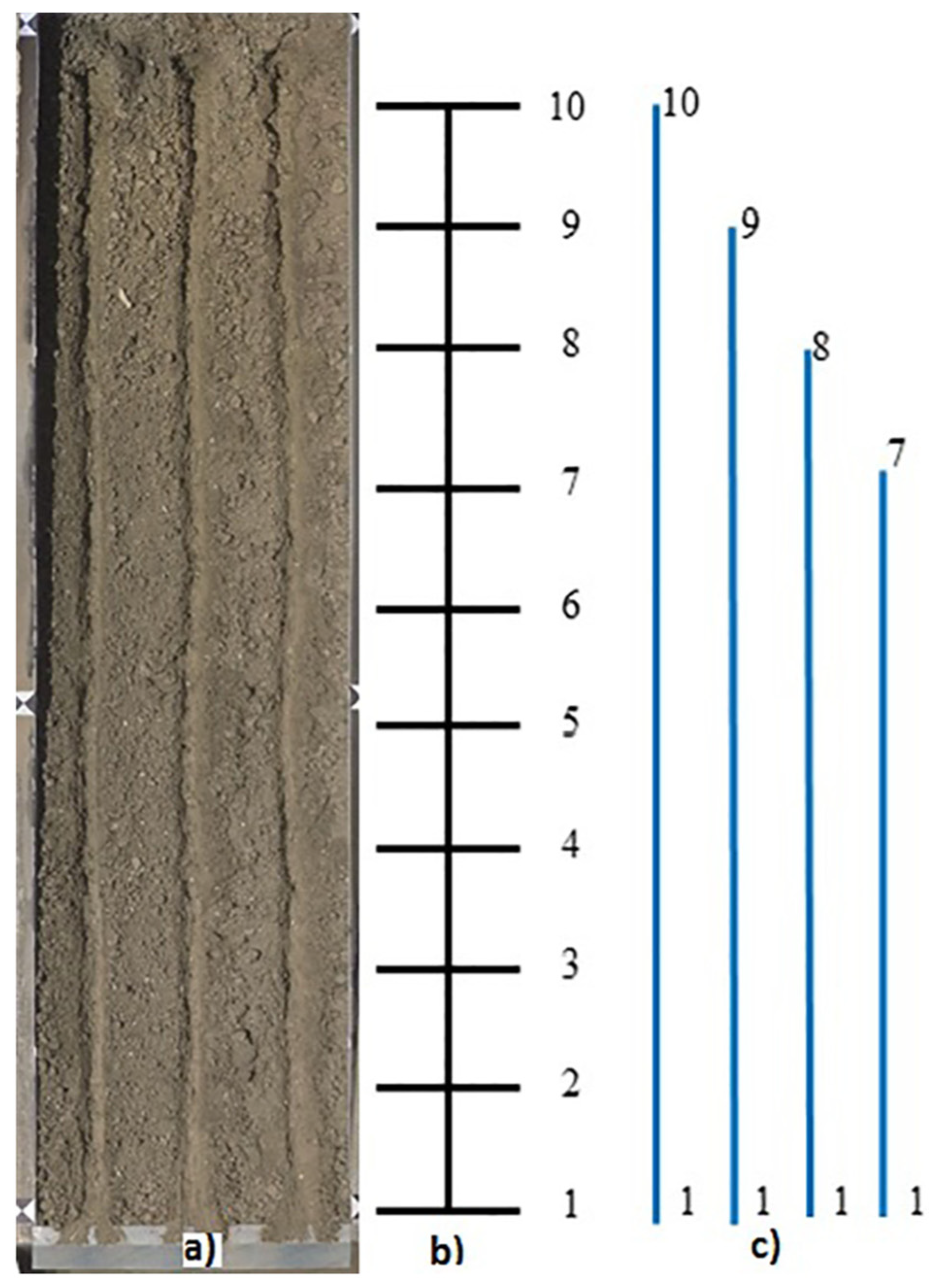
2.1. The Experimental Plots and Measurements

A plot, 2 m wide and 7 m long (Figure 1), located in the experimental area of the Department of Agriculture, Food and Forest Sciences of the University of Palermo, was used to carry out the experiments.

The plot was prepared with three different profiles (concave, convex and uniform) (Figure 1) using a mean plot slope s_p of 18%. In particular, for the concave and convex profiles, the plot was divided into two 3.27 m long parts, and two slope values (12 and 24%) were set up to obtain a mean value of 18% (Figure 2). The soil was a clay loam characterized by 32.7%, 30.9% and 36.4% of clay, silt, and sand, respectively.

For all the profile shapes, soil was manually hoed and raked and then compacted by a woody bar. The bulk density of the soil was determined by sampling the soil, using a metal cylinder of known volume, and determining its weight after drying. A uniform soil moisture condition for all the experiments was achieved by wetting the soil until infiltration stopped. Then, rills were manually incised along the maximum slope direction of the plot and were shaped using a clear flow discharge of 0.1 L s⁻¹, applied for 3 min. The rills had the same longitudinal profile as the plot. For each rill, nine longitudinal segments, bounded by two cross-sections spaced 0.624 m apart (Figure 3), were determined.

A constant clear inflow discharge, ranging from 0.18 to 0.63 L s⁻¹, was used for the experiments.

Measurements of water depth h, cross-section area σ, wetted perimeter C, bed slope s, and flow velocity V were carried out for rill reaches (i.e., the channel between a given measured cross-section and the rill end) on uniform (99 reaches), concave (71 reaches), and convex (72 reaches) rills. The indirect measurements of Reynolds number Re = V h/ν_k, in which ν_k is the kinematic viscosity, Froude number F = V/√(g h), in which g is the acceleration due to gravity, and Darcy–Weisbach friction factor f = 8 gRs /V², where R is the hydraulic radius, were also obtained.

For each experimental run, a 3D-DTM of the plot area was built from a set of 70 photographs using a 3D-photo reconstruction technique with the image-processing software Agisoft Photoscan Professional (Version 1.1.6, Agisoft, St. Petersburg, Russia). The slope gradient of each rill segment was determined using the rill thalweg imaged by the 3D-DTM. The slope of each rill reach was calculated by averaging the values measured in the considered reach.

The mean water depth h and the mean hydraulic radius R in the reach were determined using the method developed by Di Stefano et al. [36]. This method couples an accurate ground survey of the rill channel, obtained by close-range photogrammetry, with the survey of the water tracks inside the channel marked by a dye solution. The measured water depths and geometric cross-sections obtained by the 3D-DTM, at a distance interval of 6.2 cm within the reach, were used to calculate the values of the hydraulic cross-section area σ and wetted perimeter C in the reach and the values of h and R using the following equations [36]:

$$h=\frac{{{\displaystyle \sum }}_{i=2}^{N-1}\left(\frac{{\sigma }_1}{2}+{\sigma }_i+\frac{{\sigma }_N}{2}\right)}{{{\displaystyle \sum }}_{i=2}^{N-1}\left(\frac{w_1}{2}+w_i+\frac{w_N}{2}\right)}$$

(1)

$$R=\frac{{{\displaystyle \sum }}_{i=2}^{N-1}\left(\frac{{\sigma }_1}{2}+{\sigma }_i+\frac{{\sigma }_N}{2}\right)}{{{\displaystyle \sum }}_{i=2}^{N-1}\left(\frac{C_1}{2}+C_i+\frac{C_N}{2}\right)}$$

(2)

in which w is the surface width and N is the number of the cross-sections in the reach.

A methylene blue solution was applied as a dye tracer to measure the flow velocity [28,37,38,39,40]. The measured surface velocity was converted to the mean flow velocity V by a correction factor of 0.8 [41,42,43].

For four rills of each profile shape, Digital Elevation Models (DEMs) at the ends of the shaping phase (D1) and the experimental runs (D2) were obtained from the 3D-DTM. The DEM of the difference (DoD) between D2 and D1 was used to measure the scour depth values inside the whole rill channel and calculate the total eroded rill volume RV. Considering that the minimum level of detection of the used DEMs was ±0.005 m, variations of bed elevation in the range ±0.005 m were not detectable.

Finally, for the same rills, the scour depth values SD were measured, at 0.005 m intervals along the rill thalweg, as the difference in height between the longitudinal profiles at the end of the shaping phase (D1) and at the end of the experimental runs (D2) (an example for one rill with a convex profile shape is plotted in Figure 4). For each rill, the mean scour depth SD_m was also calculated as the mean of the SD values.

2.2. The Rill Flow Resistance Equation

For an open channel flow, the local flow velocity profile v(y) along a given vertical is represented by the following functional relationship [44,45,46]:

$$\phi \left(\frac{dv}{dy},y, h, d, u_{*}, s, \rho , \mu , g\right)=0$$

(3)

where φ is a functional symbol, v is the local velocity, y is the distance from the bottom, d is a characteristic bed particle diameter, u_*= √(g R s) is the shear velocity, ρ is the water density and μ is the dynamic water viscosity.

Applying the Π-Theorem of the dimensional analysis and using as dimensional independent variables y, u_* and μ, Equation (3) can be expressed by the following dimensionless functional relationship [30]:

$$\frac{y}{u_{*}}\frac{dv}{dy}={\phi }_1\left(\frac{h}{d},s,\frac{u_{*}y}{{\nu }_k},Re,F\right)$$

(4)

in which φ₁ is a functional symbol.

Hypothesizing the Incomplete Self-Similarity in u_*y/ν_k [25,47,48,49,50], neglecting the influence of Re (turbulent flow regime) and considering that the flow Froude number accounts also for the ratio h/d [26], the integration of Equation (4) yields to the following velocity profile:

$$\frac{v}{u_{*}}=\mathsf{\Gamma }\left(s,F\right) {\left(\frac{u_{*} y}{{\upsilon }_k}\right)}^{\delta }$$

(5)

where Γ(s, F) is a function to be defined by velocity measurements and the exponent δ is calculated by the following theoretical equation [51,52]

$$\delta =\frac{1.5}{\ln Re}$$

(6)

The following expression of the Darcy–Weisbach friction factor f is deduced [25,48,53] by integrating Equation (5):

$$f=8 {\left[\frac{2^{1-\delta } \mathsf{\Gamma } R{e}^{\delta }}{\left(\delta +1\right) \left(\delta +2\right)}\right]}^{-2/\left(1+\delta \right)}$$

(7)

From the velocity profile (Equation (5)) the following estimate Γ_v of Γ function [25,53] is obtained by setting equal to α h the distance y at which the local velocity is equal to the cross-section average velocity V:

$${\mathsf{\Gamma }}_v=\frac{V}{u_{*}{\left(\frac{u_{*}\alpha h}{{\nu }_k}\right)}^{\delta }}$$

(8)

The coefficient α, which is less than 1, takes into account that both V is located below the water surface and the mean velocity profile in the cross-section is considered. The coefficient α has to be calculated by the following theoretical relationship deduced by Ferro [25]:

$$\alpha ={\left[\frac{2^{1-\delta } }{\left(\delta +1\right) \left(\delta +2\right)}\right]}^{1/\delta }$$

(9)

For this investigation α varied in a narrow range and the mean value of 0.124 was assumed. Considering that, according to Equation (5), Γ theoretically depends only on s and F [26,54], Γ_v can be estimated using the following power equation:

$${\mathsf{\Gamma }}_v=a \frac{F^b}{s^c}$$

(10)

where a, b and c are coefficients to be determined from experimental measurements.

3. Results

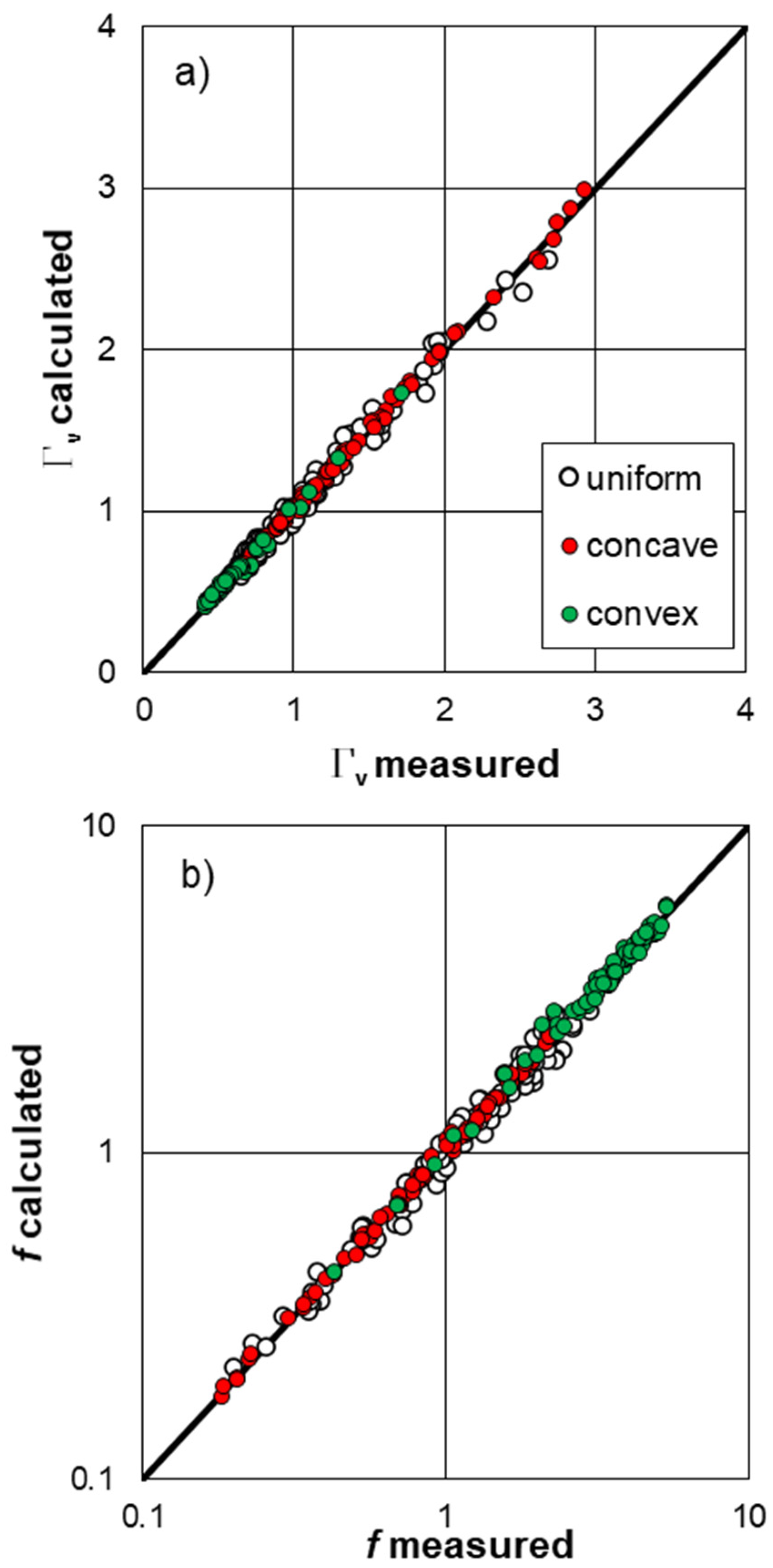
3.1. Rill Flow Resistance for Different Profile Shapes

The experimental runs were carried out for Reynolds numbers corresponding to turbulent flow (2764 ≤ Re ≤ 11015 for the uniform profile, 2282 ≤ Re ≤ 14346 for the concave one, and 2486 ≤ Re ≤ 9487 for the convex one) and for Froude number values corresponding to subcritical and supercritical flow conditions (0.54 ≤ F ≤ 1.70 for the uniform profile, 0.64 ≤ F ≤ 1.63 for the concave one, and 0.44 ≤ F ≤ 1.71 for the convex one) (Figure 5). In other words, the investigated ranges of Re and F are very similar for the three different profiles.

Using all the 242 measurements, i.e., neglecting the influence of the profile shape, Equation (10) was calibrated obtaining the following relationship:

$${\mathsf{\Gamma }}_v=0.4322 \frac{F^{1.0857}}{{\mathrm{s}}^{0.5235}}$$

(11)

characterized by a coefficient of determination equal to 0.9894. The comparison between the 242 measured Γ_v values, obtained by Equation (8) and those calculated applying Equation (11) is plotted in Figure 6a.

Introducing Equation (11) into Equation (7), the following flow resistance law was obtained:

$$f=8{\left[\frac{\left(\delta +1\right) \left(\delta +2\right)}{2^{1-\delta } R{e}^{\delta }0.4322}\frac{s^{0.5235}}{F^{1.0857}}\right]}^{2/\left(1+\delta \right)}$$

(12)

A good agreement, characterized by a root mean square error RMSE equal to 0.1743, between the measured Darcy–Weisbach friction factor values and those calculated by Equation (12) was detected (Figure 6b), even if Equation (12) tended to slightly overestimate the f values for the uniform profile. The friction factor values calculated by Equation (12) were characterized by errors less than or equal to ±20% for 96.3% of cases and less than or equal to ±10% for 78.5% of cases. Figure 6 highlights that the f measurements obtained for the convex profile covered a different range than those obtained from the uniform and concave profiles. Different characteristics of the convex profile are also revealed by the frequency distributions of the hydraulic variables F, f, s and V plotted in Figure 7.

As this analysis showed that profile shape influences flow characteristics, the theoretical flow resistance law was calibrated for each investigated condition.

Table 1. Values of a, b and c coefficients of Equation (10) obtained for the uniform, concave, and convex profiles.

Profile Shape	a	b	c
Uniform	0.4419	1.0127	0.5224
Concave	0.4025	1.1084	0.5469
Convex	0.5187	1.0437	0.3795

lists the a, b and c coefficients of Equation (10) obtained for the uniform, concave, and convex profiles.

Figure 8a shows the comparison between the measured Γ_v values obtained by Equation (8) and those calculated applying Equation (10), with the specific a, b and c coefficients (Table 1) for the different profiles. The coefficient of determination of the obtained relationships is equal to 0.9812, 0.9979 and 0.9882 for the uniform, concave, and convex profiles, respectively.

Figure 8b shows good agreement, characterized by a RMSE equal to 0.1234, between the measured values of the Darcy–Weisbach friction factor and those calculated by Equations (7) and (10), with a, b and c coefficients obtained for each profile shape. In this case, the calculated friction factor values are characterized by errors always less than or equal to ±20% and less than or equal to ±10% for 86.8% of cases.

Moreover, to study the influence of profile shape on rill flow resistance, the additive method of shear stresses [55], already used to investigate the effects of sediment transport for rills [29,56], and of riparian vegetation for a vegetated channel [57], was applied. In particular, the Darcy–Weisbach friction factor, f_mor, corresponding to the effect of the profile on flow resistance, was calculated as the difference f-f_u between the measured f value of the concave or convex profile and that of, f_u, calculated for the uniform profile in the same hydraulic conditions (Equations (7) and (10), with a, b and c coefficients obtained for the uniform profile). This f_mor value is almost equal to zero for 9.9% (concave) and 4.2% (convex) of the measured values. The ratio f_mor/f varies from 0.68 to 14.6% for concave profile and from 3.4 to 26.9% for convex profile (Figure 9).

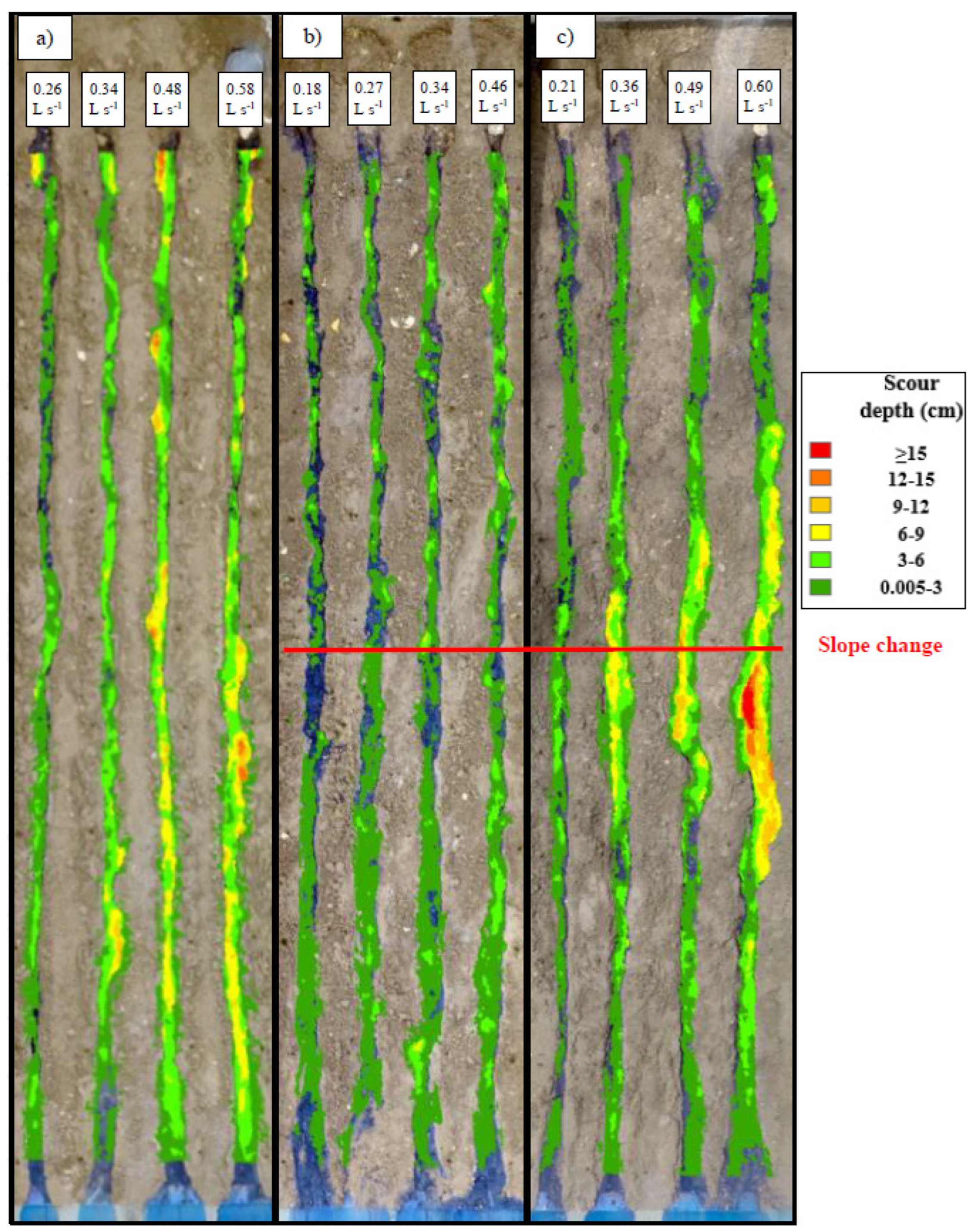
3.2. Analysis of Rill Scour Depth and Eroded Volume for Different Profile Shapes

Figure 10 shows the DoD obtained for the uniform (a), concave (b) and convex (c) profiles were characterized by comparable ranges of flow discharge (0.26–0.58 L s⁻¹ for uniform, 0.18–0.46 L s⁻¹ for concave, and 0.21–0.60 L s⁻¹ for convex profiles). This figure clearly shows that the concave profile is characterized by scour depth values (ranging from 0.005 to 0.08 m) lower than those of uniform (0.005–0.153 m) and convex (0.005–0.176 m) profiles.

For all three investigated profile shapes, Figure 10 also shows that rills are generally scoured by flow. The blue areas of this figure identify rill zones where the variation of bed elevation is lower than the minimum level of detection (±0.005 m), or lack variation. Moreover, for the convex profile, the scour is concentrated downstream of the slope change, while for uniform and concave profiles, it is uniformly distributed.

The knowledge of the scour depth values obtained by the DoDs allows calculation of the total eroded volume RV. Figure 11 shows the comparison between the applied discharge Q and RV using an example of four rills analysed for each profile. The evident trend, as expected, is that RV increases with Q for all the investigated profiles. Finally, for the uniform, concave, and convex profiles, the sum of the four RV values resulted in 0.0644, 0.0271 and 0.0654 m³, respectively.

For the forementioned four experimental runs for each profile shape, the frequency distribution of the scour depth values SD was plotted in Figure 12. This figure highlights that scour depth, measured in corresponding rill thalwegs, has a generally increasing trend with discharge for all investigated profile shapes.

Figure 13 shows the frequency distribution of the SD/SD_m ratio for the investigated discharges. This figure demonstrates that the variable SD/SD_m can be considered independent of discharge.

Figure 14 shows the empirical frequency distribution of SD/SD_m for each profile shape, using an example for a single discharge value (≈0.35 L s⁻¹). The overlapping of the three distributions suggested that SD/SD_m does not depend on profile shape.

The relationship between SD_m and the discharge was determined for each profile shape (Figure 15). The mean scour depth increased with discharge according to a power relationship depending on the profile.

4. Discussion

4.1. Rill Flow Resistance for Different Profile Shapes

Figure 5 shows that the rill flows for the three examined profiles were characterized by comparable Reynolds numbers, while for the convex profile, they were characterized, on average, by Froude numbers lower than those related to the uniform and concave profiles, and less than 1 for 93% of cases. For the latter, the pairs (Re, F) were generally overlapped. The detected trend for Froude number confirmed that the profile shape influences the kinematic flow characteristics (Figure 7a), while the comparable Reynolds number values (Figure 5) suggest that the profile does not affect the flow regime.

Figure 7 confirmed this overlapping trend for the measured flow velocity (Figure 7d) and Froude number (Figure 7a) on uniform and concave profiles. The slope values of the concave profile were less than those of the uniform profile, while the s values of the convex profile were greater than those measured on the uniform profile (Figure 7c). For the convex profile, the occurrence of the highest slope values and the lowest velocity values can be explained by the relevant erosion phenomena. Indeed, the highest RV values detected for the convex profile at the single rill and plot scale, demonstrate that for this profile, the erosion phenomena determine a major increase of grain roughness and sediment transport that lower flow velocity and increase the Darcy–Weisbach friction factor (Figure 7b). The overlapping values of flow velocity and friction factor f for uniform and concave profiles can be explained by the similar distribution of erosion phenomena occurring in the rill channels (Figure 10a,b).

The comparison between Figure 6b and Figure 8b and the error statistics highlight that a single flow resistance equation (Equation (12)) is applicable to all investigated profiles, despite the differences highlighted by the analysis of hydraulic characteristics at reach scale. However, the f estimate is more accurate if specific calibration coefficients (a, b and c) are applied for each profile.

Figure 9 demonstrates that the ratio f_mor/f was greater than 10% for 39.1% and 69.6% of the investigated cases for the concave and convex profiles, respectively. Thus, for the examined conditions, the effect of profile shape on flow resistance can be considered relevant.

The convex profile was characterized by the highest values of the ratio f_mor/f (3.4–26.9%) (Figure 9), which demonstrates that the contribution of the component of total flow resistance due to the profile was more pronounced than for the concave profile. This result can be explained as higher eroded volumes were detected for the convex profile and f_mor accounts for sediment transport and roughness effects on the flow resistance.

4.2. Analysis of Rill Scour Depth and Eroded Volume for Different Profile Shapes

Previous studies [23,58] considered a slope value of 18% as a threshold to discriminate between the gentle (GS) and the steep slope (SS) condition. This distinction is explained as differences in hydraulic (flow depth, velocity, Reynolds number, Froude number) and sediment transport (flow transport capacity, actual sediment load) variables occur. For the SS condition, results by Nicosia et al. [58] supported the conclusion that the sediment transport capacity T_c was so high that it was not a limiting factor for the actual sediment transport, while for the GS case, the actual sediment transport could be limited by both T_c and the soil particle detachability and transportability.

For the convex profile, Figure 10c shows that the scour was concentrated, while it was evenly distributed for uniform (Figure 10a) and concave profiles (Figure 10b). In particular, the noticeable scour of the rills in convex profiles was located downstream of the slope change from a gentle (12%) to a steep (24%) slope condition, because in the upstream half of the rill, the actual sediment transport was limited by T_c, while in the downstream half, it was not. Notwithstanding, the spatial distribution of the scour was similar for uniform and concave profiles, the scour depth values of concave profiles were lower than those of uniform and convex profiles, which instead were similar (Figure 10). Consequently, also the eroded volume of the rill for the concave profile was lower than the eroded volumes for the uniform and convex profiles (Figure 11). In particular, the concave profile resulted in 57.9% less soil loss than the uniform profile. This result confirms the literature findings [2,6,7,8], which have reported 50 to 80% less soil loss from concave hillslopes than from uniform slopes.

Figure 11 also shows that increasing values of flow discharge determine a higher RV. This result agrees with that obtained by Di Stefano et al. [56] who found that when discharge increased, the contribution of sediment transport to flow resistance and the eroded rill volume also increased.

The results shown in Figure 13 and Figure 14 suggest that SD/SD_m was independent of discharge and profile shape, respectively. In other words, the mean value SD_m accounted for the effects of both discharge and profile shape on scour depth.

Finally, Figure 15 demonstrates that profile shape determined a different increasing relationship between mean scour depth along the rill thalweg and discharge. The mean scour depth for the uniform profile was always higher than that obtained for the convex profile. Instead, the total eroded volume obtained for the uniform profile was slightly lower than that obtained for the convex profile. This result can be explained as the DoD information accounts for the spatial distribution of scour depth, while SD_m represents the mean value of measurements performed along a single linear flow path.

5. Conclusions

In this paper, the effect of the rill profile on flow resistance law was evaluated using measurements obtained from uniform, concave, and convex profiles.

At first, the equation to estimate the velocity profile parameter Γ was calibrated by all the available measurements and an accurate estimate of the Darcy–Weisbach friction factor (Equation (12)) was obtained. Then, to assess the influence of each profile on flow resistance law, the equation to estimate Γ was also calibrated when the data for each profile shape was distinguished. This choice determined an appreciable improvement of the friction factor estimate.

The Darcy–Weisbach friction factor corresponding to the effect of the profile on flow resistance, varied from 0.68 to 14.6% of the overall f factor for the concave profile, and from 3.4 to 26.9% of f for the convex profile.

The developed analysis also showed that for convex profiles, scour was concentrated downstream of the slope change, while for uniform and concave profiles, it was uniformly distributed. Furthermore, the scour depth measured in the corresponding rill thalwegs, had a generally increasing trend with discharge for all investigated profiles.

The total eroded volume for the concave profile was lower than those obtained for uniform and convex profiles and was characterized by being 57.9% less than for the uniform profile.

Finally, the analysis indicated that the mean value of scour depth in the rill thalweg accounted for the effects of both discharge and profile shape, and increases with increased discharge according to a relationship varying with the profile shape.

The main limitations of the study are the use of a single soil type and one mean plot slope. These can be overcome by other experiments using different soils and values of mean plot slope.

The present investigation highlights a markedly less soil loss from concave slopes than from either uniform or convex slopes. Moreover, the proposed approach allows estimating rill flow velocity, which is an essential component of process-based soil erosion models.

References

1. Liu, B.Y.; Nearing, M.A.; Risse, L.M. Slope Gradient Effects on Soil Loss for Steep Slopes. Trans. ASAE 1994, 37, 1835–1840. [Google Scholar] [CrossRef]
2. Rieke-Zapp, D.; Nearing, M.A. Slope Shape Effects on Erosion: A Laboratory Study. Soil Sci. Soc. Am. J. 2005, 69, 1463–1471. [Google Scholar] [CrossRef]
3. Young, R.A.; Mutchler, C.K. Effect of slope shape on erosion and runoff. Trans. Am. Soc. Agric. Eng. 1969, 12, 231–233. [Google Scholar]
4. Young, R.A.; Mutchler, C.K. Soil movement on irregular slopes. Water Resour. Res. 1969, 5, 1084–1089. [Google Scholar] [CrossRef]
5. Sensoy, H.; Kara, O. Slope shape effect on runoff and soil erosion under natural rainfall conditions. iForest 2014, 7, 110–114. [Google Scholar] [CrossRef] [Green Version]
6. Jeldes, I.A.; Drumm, E.C.; Yoder, D.C. Design of Stable Concave Slopes for Reduced Sediment Delivery. J. Geotech. Geoenviron. Eng. 2015, 141, 04014093. [Google Scholar] [CrossRef]
7. Williams, R.D.; Nicks, A.D. Using CREAMS to simulate filter strip effectiveness in erosion control. J. Soil Water Conserv. 1988, 43, 108–112. [Google Scholar]
8. Hancock, G.R.; Loch, R.J.; Willgoose, G.R. The design of post-mining landscapes using geomorphic principles. Earth Surf. Process. Landf. 2003, 28, 1097–1110. [Google Scholar] [CrossRef]
9. Mombini, A.; Amanian, N.; Talebi, A.; Kiani-Harchegani, M.; Rodrigo-Comino, J. Surface roughness effects on soil loss rate in complex hillslopes under laboratory conditions. Catena 2021, 206, 105503. [Google Scholar] [CrossRef]
10. Frankl, A.; Stal, C.; Abraha, A.; Nyssen, J.; Rieke-Zapp, D.; De Wulf, A.; Poesen, J. Detailed recording of gully morphology in 3D through image-based modelling. Catena 2015, 127, 92–101. [Google Scholar] [CrossRef] [Green Version]
11. Javernick, L.; Brasington, J.; Caruso, B. Modeling the topography of shallow braided rivers using Structure-from-Motion photogrammetry. Geomorphology 2014, 213, 166–182. [Google Scholar] [CrossRef]
12. Seiz, S.M.; Curless, B.; Diebel, J.; Scharstein, D.; Szeliski, R. A comparison an evaluation of multi-view stereo reconstruction algorithms. In Proceedings of the 2006 IEEE Computer Society Conference on Computer Vision and Pattern Recognition (CVPR’06), New York, NY, USA, 17–22 June 2006. [Google Scholar]
13. Di Stefano, C.; Ferro, V.; Palmeri, V.; Pampalone, V. Measuring rill erosion using structure from motion: A plot experiment. Catena 2017, 156, 383–392. [Google Scholar] [CrossRef]
14. Mutchler, C.K.; Young, R.A. Soil detachment by raindrops. In Present and Prospective Technology for Prediction Sediment Yields and Sources; USDAARS Publication ARS-S-40: Beltsville, MD, USA, 1975; pp. 113–117. [Google Scholar]
15. Zhang, P.; Tang, H.; Yao, W.; Zhang, N.; Xizhi, L.V. Experimental investigation of morphological characteristics of rill evolution on loess slope. Catena 2016, 137, 536–544. [Google Scholar] [CrossRef]
16. Bagarello, V.; Ferro, V. Plot-scale measurements of soil erosion at the experimental area of Sparacia (southern Italy). Hydrol. Process. 2004, 18, 141–157. [Google Scholar] [CrossRef]
17. Bagarello, V.; Ferro, V. Analysis of soil loss data from plots of different length for the Sparacia experimental area, Sicily, Italy. Byosyst. Eng. 2010, 105, 411–422. [Google Scholar] [CrossRef]
18. Govers, G.; Giménez, R.; Van Oost, K. Rill erosion: Exploring the relationship between experiments, modeling and field observations. Earth Sci. Rev. 2007, 8, 87–102. [Google Scholar] [CrossRef]
19. Bruno, C.; Di Stefano, C.; Ferro, V. Field investigation on rilling in the experimental Sparacia area, South Italy. Earth Surf. Process. Landf. 2008, 33, 263–279. [Google Scholar] [CrossRef]
20. Bagarello, V.; Di Stefano, C.; Ferro, V.; Pampalone, V. Establishing a soil loss threshold for limiting rilling. J. Hydrol. Eng. 2015, 20, C6014001. [Google Scholar] [CrossRef]
21. Di Stefano, C.; Ferro, V.; Pampalone, V.; Sanzone, F. Field investigation of rill and ephemeral gully erosion in the Sparacia experimental area, South Italy. Catena 2013, 101, 226–234. [Google Scholar] [CrossRef]
22. Di Stefano, C.; Ferro, V.; Pampalone, V. Modeling rill erosion at the Sparacia experimental area. J. Hydrol. Eng. 2015, 20, C5014001. [Google Scholar] [CrossRef]
23. Peng, W.; Zhang, Z.; Zhang, K. Hydrodynamic characteristics of rill flow on steep slopes. Hydrol. Process. 2015, 29, 3677–3686. [Google Scholar] [CrossRef]
24. Iradukunda, P.; Bwambale, E. Reservoir sedimentation and its effect on storage capacity–A case study of Murera reservoir, Kenya. Cogent Eng. 2021, 8, 1. [Google Scholar] [CrossRef]
25. Ferro, V. New flow resistance law for steep mountain streams based on velocity profile. J. Irrig. Drain. Eng. 2017, 143, 1–6. [Google Scholar] [CrossRef]
26. Ferro, V. Assessing flow resistance in gravel bed channels by dimensional analysis and self-similarity. Catena 2018, 169, 119–127. [Google Scholar] [CrossRef]
27. Di Stefano, C.; Ferro, V.; Palmeri, V.; Pampalone, V. Flow resistance equation for rills. Hydrol. Process. 2017, 31, 2793–2801. [Google Scholar] [CrossRef]
28. Di Stefano, C.; Ferro, V.; Palmeri, V.; Pampalone, V. Testing slope effect on flow resistance equation for mobile bed rills. Hydrol. Process. 2018, 32, 664–671. [Google Scholar] [CrossRef]
29. Di Stefano, C.; Nicosia, A.; Palmeri, V.; Pampalone, V.; Ferro, V. Comparing flow resistance law for fixed and mobile bed rills. Hydrol. Process. 2019, 33, 3330–3348. [Google Scholar] [CrossRef]
30. Di Stefano, C.; Nicosia, A.; Palmeri, V.; Pampalone, V.; Ferro, V. Estimating flow resistance in steep slope rills. Hydrol. Process. 2021, 35, e14296. [Google Scholar] [CrossRef]
31. Di Stefano, C.; Nicosia, A.; Palmeri, V.; Pampalone, V.; Ferro, V. Rill flow resistance law under equilibrium bed-load transport conditions. Hydrol. Process. 2019, 33, 1317–1323. [Google Scholar] [CrossRef]
32. Ferro, V.; Nicosia, A. Comment on “Rill erosion processes on steep colluvial deposit slope under heavy rainfall in flume experiments with artificial rain by F. Jiang et al.”. Catena 2020, 185, 103–793. [Google Scholar] [CrossRef]
33. Nicosia, A.; Di Stefano, C.; Pampalone, V.; Palmeri, V.; Ferro, V.; Nearing, M.A. Testing a new rill flow resistance approach using the water erosion prediction project experimental database. Hydrol. Process. 2019, 33, 616–626. [Google Scholar] [CrossRef]
34. Palmeri, V.; Pampalone, V.; Di Stefano, C.; Nicosia, A.; Ferro, V. Experiments for testing soil texture effects on flow resistance in mobile bed rills. Catena 2018, 171, 176–184. [Google Scholar] [CrossRef]
35. Carollo, F.G.; Di Stefano, C.; Nicosia, A.; Palmeri, V.; Pampalone, V.; Ferro, V. Flow resistance in mobile bed rills shaped in soils with different texture. Eur. J. Soil Sci. 2021, 72, 2062–2075. [Google Scholar] [CrossRef]
36. Di Stefano, C.; Nicosia, A.; Pampalone, V.; Palmeri, V.; Ferro, V. New technique for measuring water depth in rill channels. Catena 2019, 181, 104090. [Google Scholar] [CrossRef]
37. Line, D.E.; Meyer, L.D. Flow velocities of concentrated runoff along cropland furrows. Trans. ASAE 1988, 31, 1435–1439. [Google Scholar]
38. Govers, G. Relationship between discharge, velocity and flow area for rills eroding loose, non-layered materials. Earth Surf. Process. Landf. 1992, 17, 515–528. [Google Scholar] [CrossRef]
39. Abrahams, A.D.; Li, G.; Parsons, A.J. Rill hydraulics on a semiarid hillslope, southern Arizona. Earth Surf. Process. Landf. 1996, 21, 35–47. [Google Scholar] [CrossRef]
40. Di Stefano, C.; Nicosia, A.; Palmeri, V.; Pampalone, V.; Ferro, V. Dye-tracer technique for rill flows by velocity profile measurements. Catena 2020, 185, 104313. [Google Scholar] [CrossRef]
41. Luk, S.H.; Merz, W. Use of the salt tracing technique to determine the velocity of overland flow. Soil Technol. 1992, 5, 289–301. [Google Scholar]
42. Li, G.; Abrahams, A.D. Effect of salting sediment load on the determination of the mean velocity of overland flow. Water Resour. Res. 1997, 33, 341–347. [Google Scholar] [CrossRef]
43. Zhang, G.; Luo, R.; Cao, Y.; Shen, R.; Zhang, X.C. Correction factor to dye-measured flow velocity under varying water and sediment discharges. J. Hydrol. 2010, 389, 205–213. [Google Scholar] [CrossRef]
44. Barenblatt, G.I. Dimensional Analysis; Gordon &Breach, Science Publishers Inc.: Amsterdam, The Netherlands, 1987. [Google Scholar]
45. Barenblatt, G.I. Scaling laws for fully developed turbulent shear flows, part 1, Basic hypothesis and analysis. J. Fluid Mech. 1993, 248, 513–520. [Google Scholar] [CrossRef]
46. Ferro, V. Applying hypothesis of self-similarity for flow-resistance law of small-diameter plastic pipes. J. Irrig. Drain. Eng. 1997, 123, 175–179. [Google Scholar] [CrossRef]
47. Barenblatt, G.I.; Monin, A.S. Similarity laws for turbulent stratified flows. Arch. Ration. Mech. Anal. 1979, 70, 307–317. [Google Scholar] [CrossRef]
48. Barenblatt, G.I.; Prostokishin, V.M. Scaling laws for fully developed turbulent shear flows, part 2. Processing of experimental data. J. Fluid Mech. 1993, 248, 521–529. [Google Scholar] [CrossRef]
49. Butera, L.; Ridolfi, L.; Sordo, S. On the hypothesis of self-similarity for the velocity distribution in turbulent flows. Excerpta 1993, 8, 63–94. [Google Scholar]
50. Ferro, V.; Pecoraro, R. Incomplete self-similarity and flow velocity in gravel bed channels. Water Resour. Res. 2000, 36, 2761–2770. [Google Scholar] [CrossRef] [Green Version]
51. Castaing, B.; Gagne, Y.; Hopfinger, E.J. Velocity probability density functions of high Reynolds number turbulence. Phys. D 1990, 46, 177–200. [Google Scholar] [CrossRef]
52. Barenblatt, G.I. On the scaling laws (incomplete self-similarity with respect to Reynolds numbers) for the developed turbulent flows in tubes. C. R. Acad. Sci. Ser. 1991, 313, 307–312. [Google Scholar]
53. Ferro, V.; Porto, P. Applying hypothesis of self-similarity for flow resistance law in Calabrian gravel bed rivers (Fiumare). J. Hydraul. Eng. 2018, 144, 1–11. [Google Scholar] [CrossRef]
54. Ferro, V. Assessing flow resistance law in vegetated channels by dimensional analysis and self-similarity. Flow Meas. Instrum. 2019, 69, 101610. [Google Scholar] [CrossRef]
55. Yalin, M.S. Mechanics of Sediment Transport, 2nd ed.; Pergamon Press: Oxford, UK, 1977. [Google Scholar]
56. Di Stefano, C.; Nicosia, A.; Palmeri, V.; Pampalone, V.; Ferro, V. Rill flow resistance law under sediment transport. J. Soils Sediments 2022, 22, 334–347. [Google Scholar] [CrossRef]
57. Nicosia, A.; Bischetti, G.B.; Chiaradia, E.; Gandolfi, C.; Ferro, V. A Full-Scale study of Darcy-Weisbach friction factor for channels vegetated by riparian species. Hydrol. Process. 2021, 35, e14009. [Google Scholar] [CrossRef]
58. Nicosia, A.; Palmeri, V.; Pampalone, V.; Di Stefano, C.; Ferro, V. Slope threshold in rill flow resistance. Catena 2022, 208, 105789. [Google Scholar] [CrossRef]
Figure 1. View of the experimental plot with uniform (a), convex (b), and concave (c) profiles.
Water 14 00326 g001
Figure 2. Scheme of the investigated profiles.
Water 14 00326 g002
Figure 3. View of the plot area with some tested rills (a), scheme of cross-sections (b), and examples of rill reaches (c).
Water 14 00326 g003
Figure 4. Comparison, using a rill with a convex profile, between the rill thalweg at the end of the shaping phase (D1) and at the end of the experimental run (D2).
Water 14 00326 g004
Figure 5. Experimental values of Froude and Reynolds number for each profile shape.
Water 14 00326 g005
Figure 6. Comparison between the measured Γv values obtained by Equation (8) and those calculated applying Equation (11) (a) and measured Darcy–Weisbach friction factor values and those calculated by Equation (12) (b).
Water 14 00326 g006
Figure 7. Frequency distributions of Froude number (a), friction factor (b), reach slope (c) and flow velocity (d).
Water 14 00326 g007
Figure 8. Comparison between the measured Γv values obtained by Equation (8) and those calculated by Equation (10) with the shape profile-specific a, b and c coefficients (a) and measured Darcy–Weisbach friction factor values and those calculated by Equations (7) and (10) with the shape profile-specific a, b and c coefficients (b).
Water 14 00326 g008
Figure 9. Frequency distribution of the ratio fmor/f.
Water 14 00326 g009
Figure 10. DoD obtained for the uniform (a), concave (b) and convex (c) profiles.
Water 14 00326 g010
Figure 11. An example of the comparison between the applied discharge Q and the total eroded rill volume RV, for four rill channels for each profile shape.
Water 14 00326 g011
Figure 12. An example of the frequency distribution of the scour depth SD for four discharge values, for uniform (a), concave (b), and convex (c) profiles.
Water 14 00326 g012
Figure 13. An example of the frequency distribution of the SD/SDm ratio, for four discharge values, for uniform (a), concave (b), and convex (c) profiles.
Water 14 00326 g013
Figure 14. Frequency distribution of the SD/SDm ratio for a fixed value of discharge (≈0.35 L s−1).
Water 14 00326 g014
Figure 15. Relationship between mean scour depth SDm and discharge for each profile shape.
Water 14 00326 g015