Article

Influence of Negatively Buoyant Jets on a Strongly Curved Open-Channel Flow Using RANS Models with Experimental Data

Department of Civil Engineering, University of Ottawa, Ottawa, ON K1N 6N5, Canada
*
Author to whom correspondence should be addressed.
Water 2022, 14(3), 347; https://doi.org/10.3390/w14030347
Submission received: 28 December 2021 / Revised: 18 January 2022 / Accepted: 21 January 2022 / Published: 25 January 2022
(This article belongs to the Special Issue Computational Fluid Mechanics and Hydraulics)

Abstract

:
Experimental and numerical studies of flow structures in a strongly curved 135-degree laboratory flume were carried out to investigate the influence of negatively buoyant jets using the finite volume method. The performance results of three different turbulence models were investigated by comparing the numerical results with the experimental measurements. The present study demonstrates that fully 3D numerical models are capable of simulating the primary flow pattern in a strongly curved channel with the presence of a negatively buoyant jet. The comparison also shows that the k-omega SST model can satisfactorily predict some of the smaller flow features in bend flow, such as the inner bank circulation cell and the overall form of the vorticity distributions. It was found that the flow distribution and the strength of secondary flow vary due to the interaction between the jet mixing behavior and the secondary flow in the channel bend. The presence of negatively buoyant jets attenuated the development of the outer bank cell as salinity increased. In the inner bank region, flow separation was strengthened by the participation of the negatively buoyant jets.

1. Introduction

The investigation of flow structures in open channel bends is of great importance in hydraulic and environmental engineering sciences. Subjects related to super-elevation and bank erosion/shifting, bed scouring and sediment transport, migration of meanders and shear stress redistribution, as well as heat and salinity transfer have been proven to be attributed to river curvature [1]. A special feature of a curved open channel is the existence of secondary flow, resulting from the combination of lateral pressure gradients and centrifugal forces, i.e., the inclined free surface yielded transverse pressure gradient cannot balance the centrifugal force, which causes the water molecules at the bottom to move towards the inner bend and particles at the water surface to move towards the outer bend [2]. The magnitude of the cross-stream motion, which is particularly responsible for velocity redistribution and boundary shear stress, can be as much as 10–40% of the bulk streamwise velocity [3]. Although the helical flow pattern has been reported for over a century, relatively few studies have assessed how secondary flows in strongly curved bends influence the mixing of effluents [4]. To address this problem there is a need to employ fully three-dimensional models instead of conventional depth-averaged models [4,5], as well as high-resolution measurements of all velocity components.
Earlier theoretical investigations on secondary flow structure have been made mostly based on the physical properties defined by the channel geometry, such as curvature ratio (bend radius/channel width, R/B), aspect ratio (channel width/flow depth, B/H), and flow depth/bend radius (H/R = H/B × B/R) [6,7]. Later, Blanckaert and Ottevanger [8,9] employed a parameter Cf−1 H/B to assess the governing processes of flow redistribution and flow structures in bends, and they broadened the applicability range for both mildly and strongly curved channels. Moreover, many efforts have been made to take into account the influences of topography and geomorphology on curved channel flow, for instance, bathymetry or point bar and deflection angle, while aiming to enhance the understanding in order to approximate natural rivers [2,10,11,12,13,14,15,16]. However, although much work has been conducted on the details of the formation and structures of secondary flow associated with channel geometry [17,18], and even considering man-made infrastructure, very little attention has been paid to the effects of the variation of fluid properties on secondary flow.
Recently, the demands of optimizing the use of natural water bodies and mitigating environmental impacts have been emphasized, so that water pollution problems can be effectively controlled. Domestic and industrial effluents, also known as turbulent buoyant jets, are commonly discharged into rivers, estuaries, and oceans to provide for disposal in urban areas [19]. During a diffusion process, flowing fluid can easily condition the effluents, and additional complexities of the flows include the complicated interaction between effluents and the secondary flow caused by the curvature of the streamlines. It has been found that turbulence plays an important role in open channel bends. With turbulent buoyant jets, the original flow structures and turbulence in the bends will be continually disturbed by the jets in crossflow. After accumulating a certain quantity of fluids with different densities, the water properties in the bend are changed. This poses some problems compared to the bends without jets; hence, flow and turbulence characteristics need to be thoroughly examined in order to acquire reliable predictions on three-dimensional (3D) flow fields for both scientific research and practical purposes.
Flow dynamics in channel bends can be studied experimentally and numerically. Considerable effort has been put into measuring and evaluating the secondary flow in laboratory bends [1,3,20,21,22,23,24,25]. The rapid development of computer science has strengthened a series of mathematical models for hydrodynamics to better elucidate and predict the details of 3D flows in bends since the 1980s. Most of the pioneering work was carried out on closed ducts [26,27]. De Vriend [18] developed a mathematical model for the prediction of the helical flow pattern in a shallow flow conduit with respect to the Dean number. He determined that the influence of the side-wall region cannot be neglected as soon as secondary flow convection was fully developed, but instead of using any turbulence model, laminar flow condition was employed in the analysis. Leschziner & Rodi [28] developed a k-ε turbulence model to interpret the flow structure in a strongly curved open channel, and they also extended their research to closed conduits; however, due to computer storage economization, pressure values were stored two-dimensionally and streamwise diffusion was neglected. Demuren and Rodi [29] modified the model proposed by Leschziner & Rodi [29] so that the refined k-ε model could account for streamline curvatures, bed morphology and turbulent transport. Nevertheless, according to Demuren and Rodi [29] continuity errors could happen as a result of the application of “rigid lid” approximation, which prevailed in early simulations. The standard k-ε model was insufficient to solve problems within complex flows due to the isotropic eddy viscosity assumption, hence, many attempts were made to resolve the defect, either by calculating the turbulence stress from more complex stress models or by posing a substitute for the isotropic viscosity in the standard model [30]. Later, Ye and McCorquodale [3] introduced a k-ε model to overcome the anisotropic influences caused by streamline curvature, free surface, and solid walls by obtaining the turbulent viscosity from algebraic stress models (ASM) or Reynolds stress models (RSM). But given a shallow flow, the bed morphology was treated as a solid wall damping effect. Subsequently, Ruther and Olsen [31], Khosronejad et al. [32] and Zeng et al. [13] applied fully 3D Reynolds-averaged numerical simulation (RANS) model in strongly curved channels with both flat bed and moveable beds, which broadened the capability of RANS models on the scouring and deposition process of open channel bends. Zeng et al. [13] found larger discrepancies in modelled versus measured velocity in the transverse direction compared to the streamwise direction, especially for the mobile bed case. Several researchers have since developed large eddy simulation (LES) models of open channel bend flows [33,34,35,36,37,38,39], but the computational demand of LES models often precludes their use in real full-scale scenarios.
The motivation for the present work is to provide experimental data and numerical simulations on the distribution of the 3D flow velocity and turbulence in a strongly curved laboratory flume by means of a non-intrusive method. Negatively buoyant jets with different densities were continually discharged into the flow at the outer sidewall as a crossflow, and the velocity field was measured with a particle image velocimetry (PIV) system. The data were then used as a reference for model validation of three RANS models, the standard k-ε model, the non-linear k-ε model and the k-ω shear stress transport (SST) model. Experiments in this study aim to demonstrate the natural situation of effluent discharge activities. The flume employed in this study is an asymmetric 135-degree bend with a rectangular cross-sectional shape and a uniform flat channel bed. Although the reduction of topographical conditions yields more discrepancies than in natural rivers, the present study can still serve the understanding of river engineering. More specifically, four issues need to be addressed in this study. Firstly, it needs to be determined whether the occurrence of a buoyant jet will influence the secondary flow structure in a bend. Secondly, the performance of various RANS models in the simulation of a strongly curved channel flow along with the dilution problem will be evaluated. Thirdly, the influence of the density difference on flow structure will be inspected. Lastly, the turbulence structures of the flow will be inspected. Data sets obtained from the validated numerical model are used for this analysis, in order to enable a more comprehensive view of the interaction of the effluent jet with the strongly curved open channel bend flow.

2. Methodology

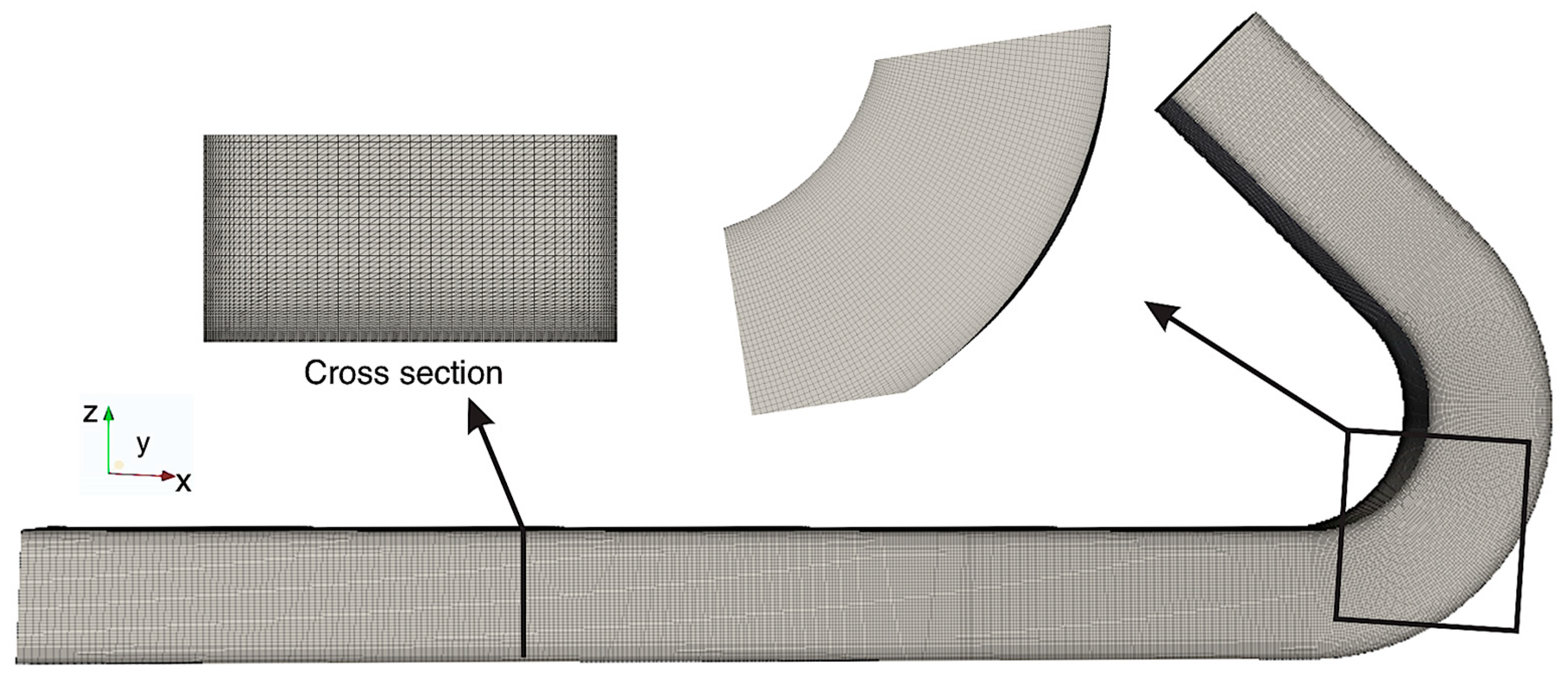
2.1. Experimental Setup and Flow Configuration

Measurements in this study were taken in a laboratory single bend flume (Figure 1), which consists of a straight entrance section with a length of 2 m and a 135-degree bend followed by a straight exit section of 0.5 m. A schematic diagram of the experimental setup is shown in Figure 1. The stream-wise, wall-normal and spanwise directions are denoted by x, y, and z, respectively; the corresponding three components of the fluctuating velocities are u, v, and w.
The width of the entire flume is uniformly B = 0.2 m, and the centerline length is 3.2 m. The bed of the flume was set horizontally, and both the bottom and the vertical sidewalls are hydraulically smooth. The radius of curvature at the centerline of the bend is R = 0.3 m. Therefore, the aspect ratio of the flume under study is R/B = 1.5, which makes it a strongly curved open channel. Water depths of all the experiments were H = 0.1 m, and the bulk velocity of the flow was 0.1 m/s. The flows in all the experiments were sub-critical flows, as the Froude number was Fr = 0. 22 < 1, and they were also fully turbulent as the Reynolds number of each test was 22,400 (Table 1).
Salt-water with salinities of 3.5, 10 and 16.5 was used for the negatively buoyant jets discharged into the channel. The nozzle was on the outer bank wall of the straight inlet section. The center of the round nozzle was 5 cm above the flume bed and the distance between nozzle center and the bend entrance was 0.55 m. Each effluent jet was discharged perpendicular to the wall, horizontally as a crossflow into the main flow. The initial velocity of each jet was kept constant using a constant head tank at a value of 0.2 m/s.

2.2. Experimental Methods

Velocity measurements were taken for all experiments using the particle image velocimetry (PIV) method. PIV is an optical measurement technique by which the velocity field of an entire interrogation plane can be measured simultaneously. A typical PIV apparatus consists of a camera (normally a digital camera with high quality CCD chips), an illumination source (a laser output device) and a synchronizer (a timing unit) to operate as an external trigger for the control of the camera and the laser. In addition, the fluids under investigation should be seeded with particles before measuring. In the present study, stereoscopic PIV (stereo-PIV) measurements were executed to mitigate the influence of distortion caused by the bend, and to obtain a measurement of the out-of-plane velocity at each measured section. Each measurement was made with a sampling frequency of 30 Hz, for an examination period of 40 s.
Measurements were performed at four different cross sections in the flume: 37, 90, 105, and 125 degrees. Data generated for one cross-sectional plane were composed by two measurements, and each PIV measurement covers half of the section. The maximum relative uncertainty of the measurements was evaluated by post-processing software along with the PIV system. The relative uncertainty values were found to be 10% in the streamwise direction, 20% for the cross-sectional velocities, and 30% in the vertical direction. However, due to the material and the geometry of the flume, strong reflection was observed at the solid boundaries. The complete image of each measurement is subdivided by the interrogation windows, then each interrogation window is evaluated by cross-correlation to generate a local vector. The details of the cross-correlation of the PIV data processing can be found in the product manual of DaVis 8.4 (refer to Adrian R [40] for more information on this procedure). The averaged resolution of each measured plane was 44 interrogation windows with the width and 22 interrogation windows with the depth. In the current setting, the PIV measurements yielded low correlations and high uncertainties in a flow layer of approximately 0.5 to 1 cm near solid boundaries.

2.3. Numerical Methods and Turbulence Models

2.3.1. Numerical Models

In the present study, the incompressible Navier-Stokes equations were solved by using the finite volume method for the liquid coupled with the volume of fluid method for the salinity distribution. All the simulations were performed with the open-source code OpenFOAM (version 7.0) via the multi-fluid turbulence solver called twoLiquidMixingFoam. The twoLiquidMixingFoam software was developed to solve problems regarding the mixing of two incompressible fluids, and it has been utilized and substantiated in many studies [41]. The implementation of the turbulence models was managed by employing different schemes for each term in the governing equations. A Eulerian scheme was used to discretize the temporal term. The gradient terms were controlled by the Gauss linear scheme, while a corrected Gauss linear scheme was used to discretize the Laplacian term. Gauss vanLeer, Gauss linear and bounded Gauss upwind schemes were assigned to the divergence terms. To interpolate values from one set of points to another, a linear scheme was used in discretization. A structured mesh (Figure 2) was used in the numerical simulations with the same geometry as in the experiments (physical domain).

2.3.2. The Standard k-ε Model

The three-dimensional flow field is obtained by solving the continuity equation and the Reynolds Averaged Navier–Stokes equations, which can be written as:
· U = 0
ρ U t + · ( ρ U U ) = · ( p r g h ) g h ρ + ( P T )
where t is time, U indicates velocity vector, and ρ is the fluid density, g is the gravity, p r g h is the hydrostatic pressure for the pressure calculations.
With the Boussinesq assumption, the turbulence stress can be expressed as:
u i u j ¯ = ν t ( U i x j + U j x i ) 2 3 k δ i j
The realizable k-ε model is used in the present simulation for the RANS model; the turbulent kinetic energy k and its dissipation rate ϵ are obtained from the following equations:
D D t ( ρ k ) = · ( ρ D k k ) + ρ G 2 3 ρ ( · u ) k ρ ϵ + S k
D D t ( ρ ϵ ) = · ( ρ D ϵ ϵ ) + C 1 ρ | S | ϵ C 2 ρ ϵ 2 k + ( ν ϵ ) 0.5 + S ϵ
ν t = C μ k 2 ϵ
C μ = 1 A 0 + A 1 k U * ϵ
The default model coefficients are C μ = 0.09 ;   C 1 = 1.44 ;   C 2 = 1.92 ;   C 3 , R D T = 0.0 ;   σ k = 1.0 ;   σ ϵ = 1.3 .

2.3.3. The Non-Linear k-ε Model (Shih Quadratic k-ε)

The turbulence kinetic energy equation is given by:
D D t ( k ) = ( D k k ) + G ϵ
and the dissipation rate by:
D D t ( ϵ ) = ( D ϵ ϵ ) + C 1 G ϵ k C 2 ϵ 2 k
the turbulence generation G is given by:
G = [ ν t ( u + ( u ) T ) τ n l ] : u
where τ n l is the non-linear stress.

2.3.4. The k-ω SST (Shear Stress Transport) Model

The complete formulation of the k-ω SST model used in the current paper is given as:
( ρ k ) t + ( ρ U i k ) x i = min ( G , c 1 β * k ω ) β * ρ k ω + x i [ ( μ + α k i μ t ) k x i ]
( ρ ω ) t + ( ρ U i ω ) x i = α P ˜ k / μ t β ρ ω 2 + x i [ ( μ + α ω i μ t ) ω x i ] + 2 ( 1 F 1 ) ρ σ w 2 1 ω k x i ω x i
where the blending function F1 is defined by:
F 1 = tan h { { m i n [ m a x ( k β * ω y , 500 v y 2 ω ) , 4 ρ σ ω 2 k C D k ω y 2 ] } 4 }
With C D k w = m a x ( 2 ρ α ω 2 1 ω k x i ω x i , 10 10 ) and y is the distance to the nearest wall.
F1 is equal to zero away from the surface (k-ε model) and switches over to one inside the boundary layer (k-ω model).
The turbulent eddy viscosity is defined as follows:
v t = a 1 k m a x ( a 1 ω , S F 2 )
where S = 2 S i j S i j is the invariant measure of the strain rate and F2 is a second blending function defined by:
F 2 = tan h [ [ m a x ( 2 k β * ω y , 500 v y 2 ω ) ] 2 ]
A production limiter is used in the SST model to prevent the build-up of turbulence in stagnation regions:
S i j = 1 2 ( u j x i + u i x j )
G = μ t S 2
All constants are computed by a blend of the corresponding constants of the k-ε and the k-ω model via α = α1F + α2(1 − F) etc. The constants for this model are: β* = 0.09, α1 = 5/9, β1 = 3/40, αk1 = 0.85, σω1 = 0.5, α2 = 0.44, β2 = 0.0828, σk2 = 1, σω2 = 0.856.

2.4. Boundary Conditions and Model Setup

A stress-free rigid lid condition was adopted to produce the effect of the free surface in the present study. Simulations with rigid lid assumption have been accepted with reasonable accuracy for the RANS models if the Froude number is smaller than 0.5 and the gradient of the water’s surface can be neglected. [2,13,33]. Due to the computational capacity and the limitations of OpenFOAM, the mesh grids near the solid boundary cannot be fine enough to reach the resolvable grid size for viscous sub-layer calculation. Therefore, the wall-function approach was employed to handle the viscous sub-layer, the buffer layer and the logarithm layer on each wall boundary in the RANS simulations. Before the comparison, a mesh sensitivity analysis was conducted by using different meshes with increasing resolution in the grids, until it can provide steady results with enough accuracy. For example, Mesh 1 has 487,921 computational cells, and the number of cells increased until the correlation coefficient of a sample velocity field increases from 0.44 to 0.98. Finally, Mesh 6, which had 1592,347 cells with a correlation coefficient of 0.96, was adopted.
The labelling of the simulation runs (first column of Table 2) is as follows. The first character denotes the density difference: S3.5 means the low salinity case, S10 means the medium case, S16.5 means high salinity case and No stands for the no jet case. The number indicates the type of simulation applied: 1 represents the k-ε model, 2 represents the Non-linear k-ε models and 3 represents the k-ω SST model.

3. Results and Analysis

3.1. Model Evaluation

The performance of each numerical model was evaluated by calculating the overall difference between experimental and numerical results. Results showed that the averaged RMSEs (root mean square errors) of the simulated total velocity magnitudes were 0.029 m/s, 0.028 m/s and 0.027 m/s for the k-ε mode, the non-linear k-ε model and the k-ω SST model respectively, indicating that the 3D numerical models can provide reasonable results for the flow field within the bend.

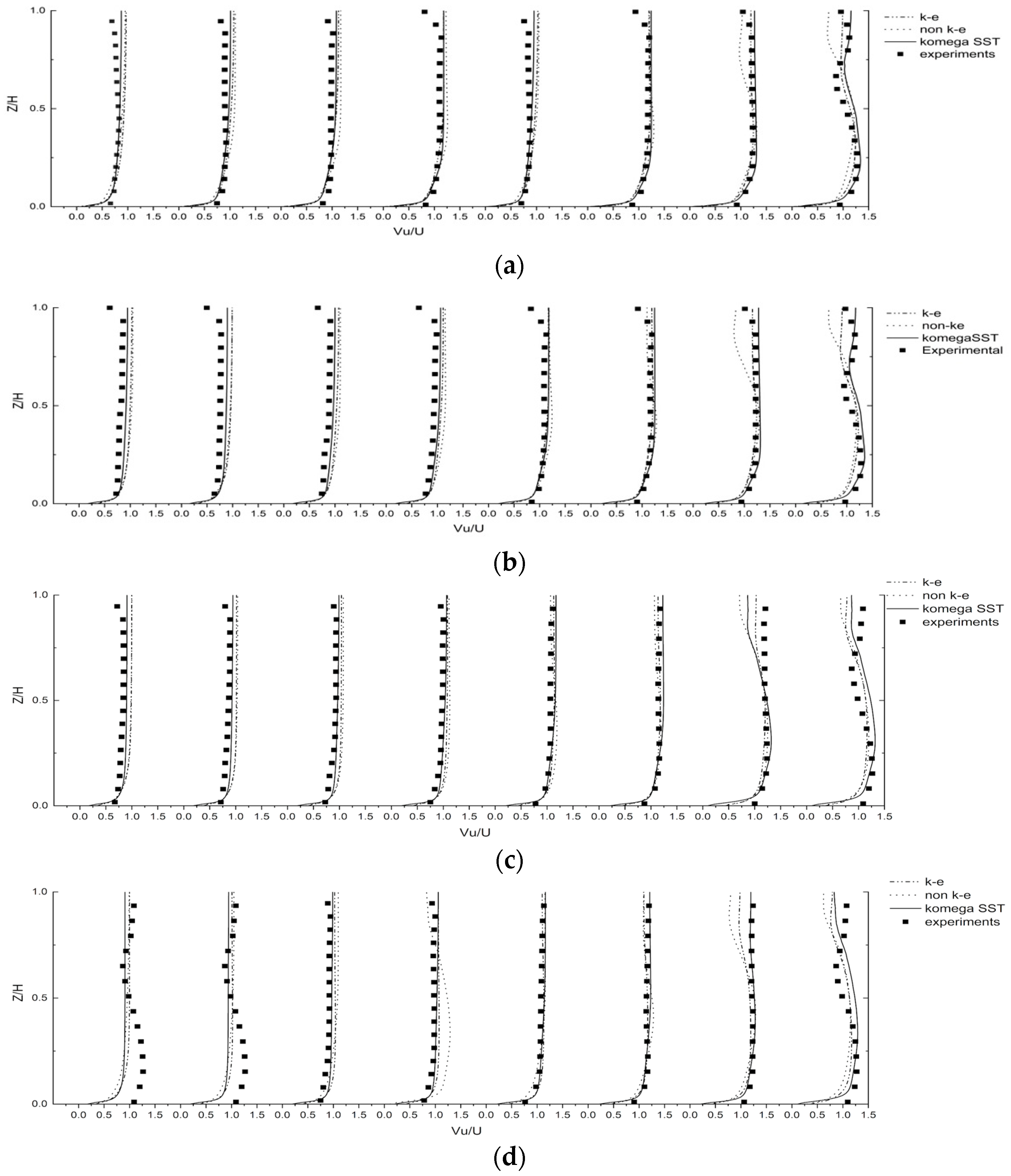
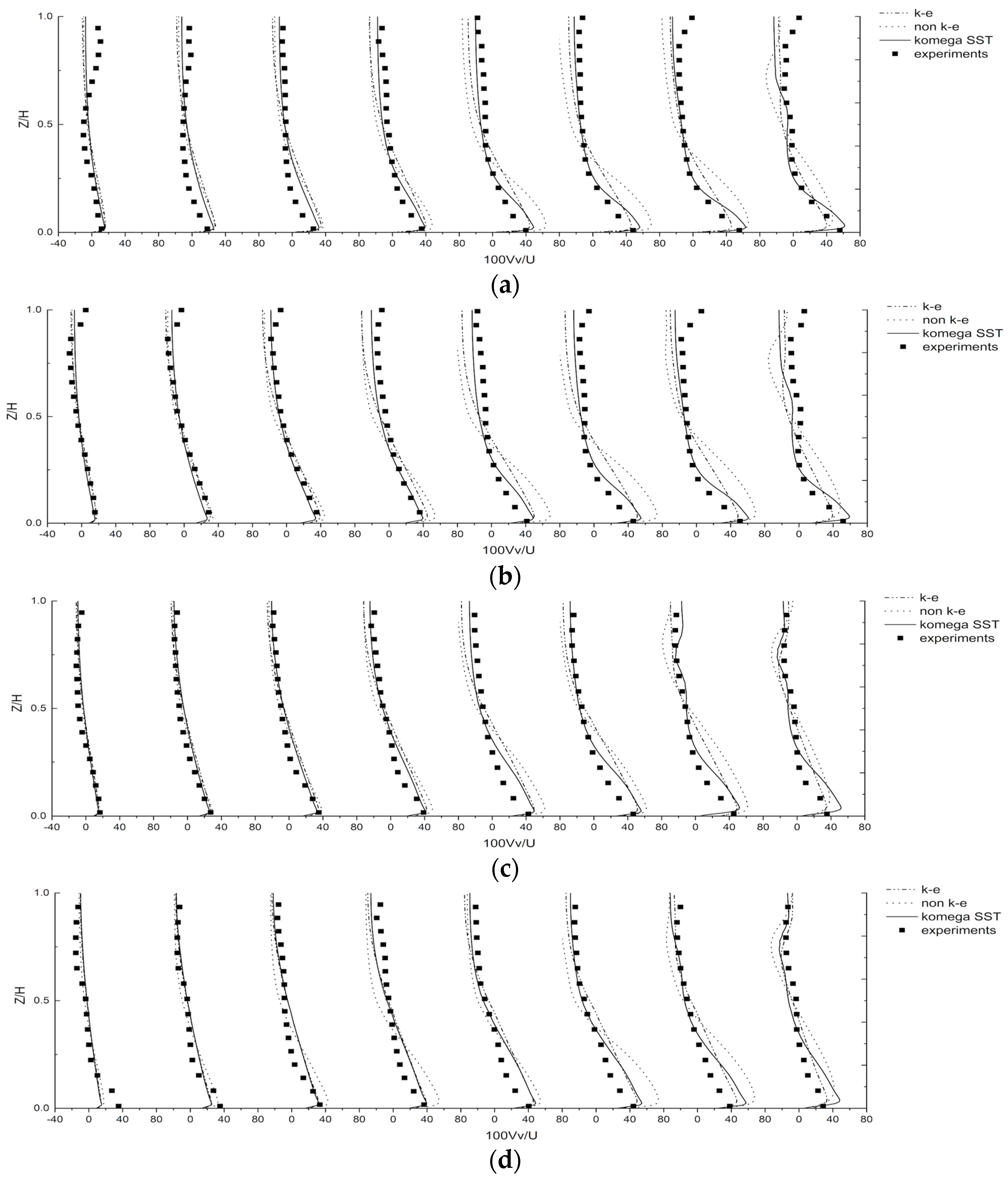
3.2. Velocity Distribution

To achieve better analysis, velocity profiles over the flow depth are shown for quantitative investigations with results of the k-ω SST model, k-εmodel and non-linear k-εmodel; specifically, transverse, vertical and streamwise velocity profiles at certain cross sections in the flow are highlighted. In the current setup of the stereo-PIV, the included angle of the two cameras inevitably changed due to the moving of the laser and the cameras during measuring different cross sections. Therefore, the resolution of the images taken from different cross sections varied slightly, which generated different mapped meshes of target flow surfaces. By avoiding the high uncertainty areas near the solid boundary, the transverse locations of the profiles are approximately 0.10 B, 0.2 B, 0.3 B, 0.4 B, 0.6 B, 0.7 B, 0.8 B and 0.9 B. Then, the time-averaged stream-wise velocities, u, and transverse velocities, v, of the experiments and numerical simulations results are shown, non-dimensionalized by the bulk velocity of the mean flow in the straight inflow channel, U.
Figure 3 compares the streamwise velocity distribution with experimental data under different jet salinities at the 90-degree section. As can be seen, the streamwise velocity profiles from the k-ω SST model agrees with the experimental results with reasonable accuracy, especially for the no-jet and low-salinity conditions (Figure 3a,b). For the highest salinity case, the streamwise velocities seem to be underestimated in relation to the lower part at the outer bank side (Figure 3d) and the upper part at the inner bank. Due to the generally formed secondary current as the flow proceeded, the velocity deformed in all three directions x, y, z, i.e., velocities did not behave according to a logarithmic distribution with depth in the bend section. Except for the center region secondary flow, there is another weak circulation cell existing at the outer bank region close to the water surface. This can be found in Figure 3, with the experimental results showing that the velocity profiles deformed in the mentioned region. Discrepancies are observed for the numerical simulations for all the cases in the outer bank region.
As can be seen from Figure 4, the agreement of the transverse velocity profiles for the medium case is quite good, but for the lower salinity case, the numerical results are of lower quality. The transverse velocities seem to be overestimated by the numerical computations at both the bottom regions and the water’s surface. However, as salinity increases, the agreement of the velocity profiles for the higher salinity cases gets better at the water’s surface of the inner bank, especially for the S = 10 case. The disagreement might be due to applying the rigid-lid assumption to the free surface, and it could also indicate that the mixing of negatively buoyant jets attenuates the spatial development of the flow structure at the inner side. Another explanation for the discrepancy can be attributed to the measurement technology in that a high intensity of reflection causes noise at the investigated boundaries.
Figure 5 shows the vertical component of the velocity profile. Weaker agreements of the vertical velocities were also found with the higher salinity case at the boundaries, and as the salinity increases, the disagreement was amplified. Despite this, it is obvious that the k-ω SST model exhibited better performance in predicting the vertical velocities in the bend under the influence of negatively buoyant jets. It can also be seen that the presence of negatively buoyant jets reverses the vertical velocity signs at the water’s surface, and the maximum value of the vertical velocities move close to the bottom as salinity increases.

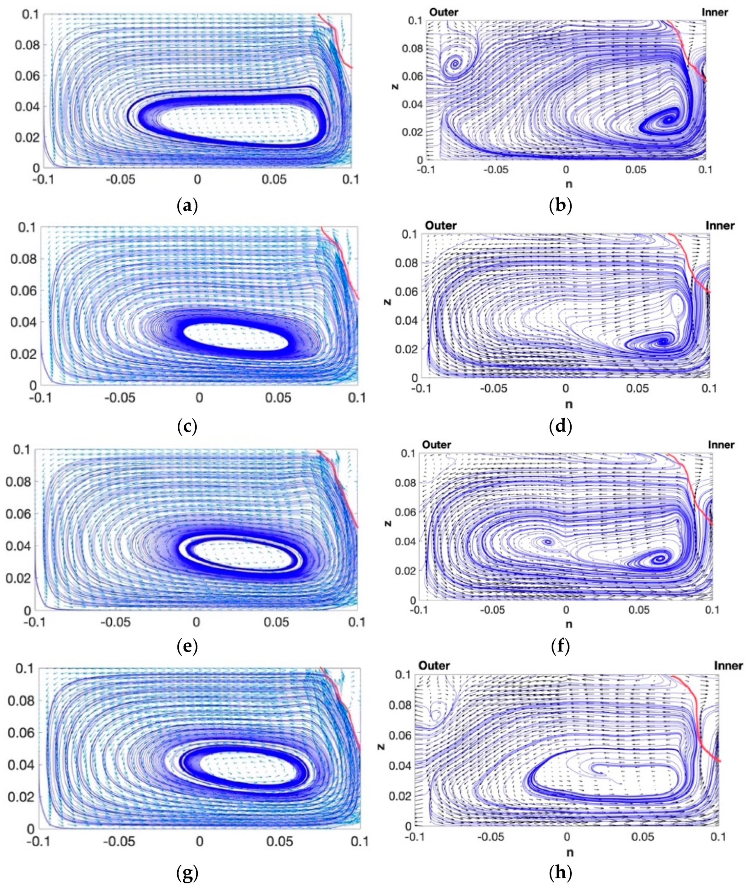
3.3. Secondary Flow Pattern

The plots of streamlines at the 90-degree section under the no-jet condition and three different salinity cases are presented in Figure 6. In this part, secondary flow properties were only compared using the results obtained by the k-ω SST model to the experimental measurements, since this model provided the best performance. As mentioned in Section 3.2, the outer bank cells under all the various scenarios were not captured by the k-ω SST model. However, the classical radial flow (also known as the main cell) towards the inner wall, which was caused by the imbalance between the centrifugal force and the lateral pressure gradient, can be seen at the 90-degree section with good agreement. As can be seen in Figure 6, the center of the main cell is moving upward to the water’s surface in both the numerical results and the measurements when salinity increases. Moreover, at the inner bank side, there are regions with adverse velocity vectors which have been widely demonstrated as separation zones. It has been reported that flow separation is promoted by the difference between the pressure gradient force caused by the streamline curvature and the inertial forces [23]. As the salinity increases, it can be found that the separation zones enlarge (marked by the red line).
To obtain better comprehension of the secondary flow, the averaged streamwise vorticities for all the scenarios considered at the 90-degree cross-sectional plane were calculated and presented in Figure 7. As shown, the positive vorticity covers most of the channel cross-section, which represents the presence of the classical helical flow in a bend. The negative values of the vorticity at the outer bank side proved the existence of the outer bank circulation cell, which has an opposite sense of rotation to the main cell. At the inner bank, negative values were also observed within a narrow region, representing the separation zones of the bend, and the flow separation behavior was strengthened as salinity increases. Furthermore, it can be seen that the high positive vorticity cores at the inner bank of the channel are retreating and shrinking towards the inner wall as salinity increases.

4. Discussion

It is commonly accepted that flow behaviors in bends should be treated with an advanced turbulence model, such as the LES models, Reynolds stress models or even DNS models. Despite the high-quality performance, time and computational costs are still the primary obstacles for widely applying these models. Although problems related to the topic of this paper are quite complex, it is worth attempting to use two-equation Boussinesq turbulence models and to determine how precise the results are.
The present paper is an experimental and numerical study on a strongly curved 135-degree open channel bend. The findings of the present study involve the influences of the mixing behavior of negatively buoyant jets on the flow distribution and secondary flow cells in the bend, which are profound in environmental engineering. One crucial advantage of the present work is the direct comparison of parameters between the high-resolution three-dimensional measurements and fully three-dimensional numerical results, which helps foster a thorough understanding in model analysis. The present results imply that flow structures, with the interaction of negatively buoyant jets in a channel bend, are distinct from the bends without jets. It also shows that the flow distribution was considerably influenced by the jets mixing behavior. In a channel bend without a jet, the size of the outer bank cell is larger than that of a channel bend with jets, while the inner bank flow separation process was enhanced with the latter cases of bends with jets. Moreover, flow redistribution in a channel bend resulting from the pressure gradient imbalance was more complicated in the presence of jets, and the effects varied with respect to each velocity component at different locations. Overall, the results demonstrate that the salinity of a negatively buoyant effluent jet will have important consequences for its interaction with secondary flow structures and associated mixing in an open channel bend.

5. Conclusions

In this study, numerical modelling of the flow pattern with the influence of negatively buoyant jets at a strongly curved open channel bend was carried out to compare the results of using fully 3D RANS turbulent models (the standard k-ε model, non-linear k-ε model, and the k-ω SST model) with the results from an experimental channel. The performance of these models was evaluated in this channel.
The key findings of the research are listed below:
  • With all the applied turbulence models, the streamwise velocities were all well predicted for the lower salinity cases. Discrepancies were found near the water’s surface at the outer bank region due to the inability of resolving the outer bank cell numerically. Reasonable agreement was obtained concerning the transverse velocities between the numerical results and the measured data. The major computational differences were observed with the vertical velocity component. Overall, the k-ω SST model exhibited the best performance in the present study. The computational errors can be attributed to the use of the isotropic eddy viscosity and the rigid-lid free surface assumption.
  • The velocity patterns in all three directions were influenced by the effect of secondary flow, which was attained in the channel bend by the experimental data and numerical simulations.
  • The overall shapes of streamlines at each salinity case are different from each other because of the interaction between the jet mixing behavior and the secondary flow in the channel bend.
  • The presence of negatively buoyant jets disturbed the development of the outer bank cell, and the influence was attenuated as salinity increased.
  • In the inner bank region, flow separation was strengthened by the participation of the negatively buoyant jets.
  • High positive streamwise vorticity cores, which represent the main circulation, were found at the inner bank, and they were pushed towards the inner bank wall as salinity increased.
The present study only focuses on RANS models. The authors suggest that other turbulence models (such as LES, RSM, etc.) are worth studying, and the alternative boundary conditions need to be further investigated. Future research objectives would also involve the influence of more types of jets, the discharge location, as well as the jets’ mixing characteristics.

Author Contributions

Conceptualization, A.M. and C.D.R.; Data curation, X.W.; Formal analysis, X.W.; Investigation, X.W.; Methodology, A.M. and C.D.R.; Project administration, A.M. and C.D.R. Supervision, A.M. and C.D.R.; Writing—original draft, X.W.; Writing—review & editing, A.M. and C.D.R. All authors have read and agreed to the published version of the manuscript.

Funding

This research received no external funding.

Institutional Review Board Statement

Not applicable.

Informed Consent Statement

Not applicable.

Data Availability Statement

Part of the data is available by the corresponding author upon request.

Conflicts of Interest

The authors declare that they have no conflict of interest.

References

  1. Chang, Y.C. Lateral Mixing in Meandering Channels; University of Iowa: Iowa City, IA, USA, 1971. [Google Scholar]
  2. Kashyap, S.; Constantinescu, G.; Rennie, C.D.; Post, G.; Townsend, R. Influence of channel aspect ratio and curvature on flow, secondary circulation, and bed shear stress in a rectangular channel bend. J. Hydraul. Eng. 2012, 138, 1045–1059. [Google Scholar] [CrossRef]
  3. Ye, J.; McCorquodale, J.A. Simulation of curved open channel flows by 3D hydrodynamic model. J. Hydraul. Eng. 1998, 124, 687–698. [Google Scholar] [CrossRef]
  4. Choi, Y.; Stewar, J.P.; Graves, R.W. Empirical Model for Basin Effects Accounts for Basin Depth and Source Location. BSSA 2005, 95, 1412–1427. [Google Scholar] [CrossRef]
  5. Song, G.C.; Seo, I.W.; Kim, Y.D. Analysis of secondary current effect in the modeling of shallow flow in open channels. Adv. Water Resour. 2012, 41, 29–48. [Google Scholar] [CrossRef]
  6. Rozovskii, I. Flow of Water in Bends of Open Channels; Academy of Sciences of the Ukrainian SSR; Israel Program for Scientific Translations: Jerusalem, Israel, 1961. [Google Scholar]
  7. Leppold, L.B.; Bagnold, R.A.; Wolman, M.G.; Brush, L.M., Jr. Flow Resistance in Sinuous or Irregular Channels: U.S. Geological Survey Professional Paper 282-D; U.S. Government Printing Office: Washington, DC, USA, 1960; pp. D111–D134.
  8. Ottevanger, W.; Blanckaert, K.; Uijttewaal, W.S.J. Processes governing the flow redistribution in sharp river bends. Geomorphology 2012, 163, 45–55. [Google Scholar] [CrossRef] [Green Version]
  9. Ottevanger, W.; Blanckaert, K.; Uijttewaal, W.S.J. A Parameter Study on Bank Shear Stresses in Curved Open Channel Flow by Means of Large-Eddy Simulation. In Proceedings of the 7th IAHR Symp. on River, Coastal and Estuarine Morphodynamics, International Association for Hydro-Environment Engineering and Research, Madrid, Spain, 6–8 September 2011; pp. 1917–1927. [Google Scholar]
  10. Engelund, F.; Skovgaard, O. On the origin of meandering and braiding in alluvial streams. J. Fluid Mech. 1973, 57, 289–302. [Google Scholar] [CrossRef]
  11. Ikeda, S.; Yamasaka, M.; Chiyoda, M. Bed topography and sorting in bends. J. Hydraul. Eng. 1987, 113, 190–204. [Google Scholar] [CrossRef]
  12. Jamieson, G.P.; Rennie, C.D. Spatial variability of three dimensional Reynolds stresses in a developing channel bend. Earth Surf. Processes Landf. 2010, 35, 1029–1043. [Google Scholar] [CrossRef]
  13. Zeng, J.; Constantinescu, G.; Blanckaert, K.; Weber, L. Flow and bathymetry in sharp open-channel bends: Experiments and predictions. Water Resour. Res. 2008, 44, W09401-n/a. [Google Scholar] [CrossRef]
  14. Kalkwijk, J.T.; De Vriend, H.J. Computation of the flow in shallow river bends. J. Hydraul. Res. 1980, 18, 327–342. [Google Scholar] [CrossRef] [Green Version]
  15. Kasvi, E.; Laamanen, L.; Lotsari, E.; Alho, P. Flow Patterns and Morphological Changes in a Sandy Meander Bend during a Flood-Spatially and Temporally Intensive ADCP Measurement Approach. Water 2017, 9, 106. [Google Scholar] [CrossRef] [Green Version]
  16. Tchobanoglous, G. Wastewater Engineering: Treatment Disposal Reuse, 2nd ed.; McGraw-Hill: New York, NY, USA, 1979. [Google Scholar]
  17. Cheng, G.C.; Farokhi, S. On turbulent flows dominated by curvature effects. J. Fluid Engrg. ASME 1992, 114, 52–57. [Google Scholar] [CrossRef]
  18. de Vriend, H. Velocity redistribution in curved rectangular channels. J. Fluid Mech. 1980, 107, 423–439. [Google Scholar] [CrossRef]
  19. Duan, J.G.; Julien, P.Y. Julien Numerical simulation of the inception of channel meandering. Earth Surf. Process. Landf. 2005, 30, 1093–1110. [Google Scholar] [CrossRef]
  20. Odgaard, A.J.; Bergs, M.A. Flow processes in a curved alluvial channel. Water Resour. Res. 1988, 24, 45–56. [Google Scholar] [CrossRef]
  21. Booij, R. Measurements and large eddy simulations of the flows in some curved flumes. J. Turbul. 2003, 4, 008. [Google Scholar] [CrossRef]
  22. Blanckaert, K.; De Vriend, H.J. Secondary flow in sharp open-channel bends. J. Fluid Mech. 2004, 498, 353–380. [Google Scholar] [CrossRef] [Green Version]
  23. Blanckaert, K. Flow separation at convex banks in open channels. J. Fluid Mech. 2015, 779, 432–467. [Google Scholar] [CrossRef]
  24. Blanckaert, K. Saturation of curvature-induced secondary flow, energy losses, and turbulence in sharp open-channel bends: Laboratory experiments, analysis, and modeling. J. Geophys. Res. 2009, 114, 432–467. [Google Scholar] [CrossRef] [Green Version]
  25. Blanckaert, K.; Graf, W.H. Momentum Transport in Sharp Open-Channel Bends. J. Hydraul. Eng. 2004, 130, 186–198. [Google Scholar] [CrossRef]
  26. Patankar, S.V.; Pratap, V.S.; Spalding, D.B. Prediction of turbulent flow in curved pipes. J. Fluid Mech. 1975, 67, 583–595. [Google Scholar] [CrossRef] [Green Version]
  27. Patankar, S.V.; Spalding, D.B. A calculation procedure for heat, mass and momentum transfer in 3-D parabolic flows. Int. J. Heat Mass Transf. 1972, 15, 1787–1806. [Google Scholar] [CrossRef]
  28. Leschziner, M.A.; Rodi, W. Calculation of strongly curved open channel flow. J. Hydraul. Div. 1979, 105, 1297–1314. [Google Scholar] [CrossRef]
  29. Demuren, A.O.; Rodi, W. Calculation of flow and pollutant dispersion in meandering channels. J. Fluid Mech. 1986, 172, 63–92. [Google Scholar] [CrossRef]
  30. Cokljat, D.; Younis, B.A. Second-Order closure study of open-channel flows. J. Hydraul. Eng. 1995, 121, 94–107. [Google Scholar] [CrossRef]
  31. Ruther, N.; Olsen, N.R.B. Three-Dimensional modeling of sediment transport in a narrow 90° channel bend. J. Hydraul. Eng. 2005, 131, 917–920. [Google Scholar] [CrossRef]
  32. Khosronejad, A.; Rennie, C.D.; Salehi Neyshabouri, A.A.; Townsend, R.D. 3D Numerical Modeling of Flow and Sediment Transport in laboratory channel bends. J. Hydraul. Eng. (ASCE) 2007, 133, 1123–1134. [Google Scholar] [CrossRef]
  33. Zhiyin, Y. Large-Eddy simulation: Past, present and the future. Chin. J. Aeronaut. 2015, 28, 11–24. [Google Scholar] [CrossRef] [Green Version]
  34. Shaheed, R.; Mohammadian, A.; Yan, X. A Review of Numerical Simulations of Secondary Flows in River Bends. Water 2021, 13, 884. [Google Scholar] [CrossRef]
  35. van Balen, W.; Blanckaert, K.; Uijttewaal, W.S.J. Analysis of the role of turbulence in curved open-channel flow at different water depths by means of experiments, LES and RANS. J. Turbul. 2010, 11, N12. [Google Scholar] [CrossRef]
  36. Van Balen, W.; Uijttewaal, W.S.J.; Blanckaer, K. Large-Eddy Simulation of a Mildly Curved Open-Channel Flow. J. Fluid Mech. 2009, 630, 413–442. [Google Scholar] [CrossRef] [Green Version]
  37. Van Balen, W.; Uijttewaal, W.S.J.; Blanckaert, K. Large-Eddy Simulation of a Curved Open-Channel Flow over Topography. Phys. Fluids 2010, 22, 1–18. [Google Scholar] [CrossRef] [Green Version]
  38. Constantinescu, G.; Kashyap, S.; Tokyay, T.; Rennie, C.D.; Townsend, R.D. Hydrodynamic Processes and Sediment Erosion Mechanisms in an Open Channel Bend of Strong Curvature with Deformed Bathymetry. J. Geophys. Res. Earth Surf. 2013, 118, 480–496. [Google Scholar] [CrossRef]
  39. Mete, K.; Constantinescu, G.; Blanckaert, K. Hydrodynamic Processes, Sediment Erosion Mechanisms, and Reynolds-Number-Induced Scale Effects in an Open Channel Bend of Strong Curvature with Flat Bathymetry. J. Geophys. Res. Earth Surf. 2013, 118, 2308–2324. [Google Scholar]
  40. Adrian, R.; Westerweel, J. Particle Image Velocimetry; Cambridge University Press: New York, NY, USA, 2011. [Google Scholar]
  41. Yan, X.; Mohammadian, A. Numerical modeling of vertical buoy- ant jets subjected to lateral confinement. J. Hydraul. Eng. 2017, 143, 04017016. [Google Scholar] [CrossRef] [Green Version]
Figure 1. Flow geometry of the experiment.
Water 14 00347 g001
Figure 2. Structured mesh for numerical simulations, also showing a detailed view of the mesh and the cross-sectional view.
Water 14 00347 g002
Figure 3. Distribution of streamwise component of velocity at 90 degrees under different jet conditions: (a) no jet, (b) S = 3.5 (c) S = 10 and (d) S = 16.5. From the left to the right is the outer bank to the inner bank.
Water 14 00347 g003
Figure 4. Distribution of transverse component of velocity at 90 degrees with different jet conditions: (a) no jet, (b) S = 3.5 (c) S = 10 and (d) S = 16.5. From left to right is the outer bank to the inner bank.
Water 14 00347 g004
Figure 5. Distribution of vertical component of velocity at 90 degrees with different jet conditions: (a) no jet, (b) S =3.5 (c) S = 10 and (d) S = 16.5. From the left to the right is the outer bank to the inner bank.
Water 14 00347 g005
Figure 6. Secondary flows at the 90 degree section under different conditions: (a,b)—No jet; (c,d)—S = 3.5; (e,f)—S = 10; (g,h)—S = 16.5. The left column figures represent the numerical results, and the right column are the experimental results.
Water 14 00347 g006
Figure 7. Vortex contour of the secondary flows under different conditions: (a,e)—No jet; (b,f)—S = 3.5; (c,g)—S = 10; (d,h)—S = 16.5. Figures in the first row represent the numerical results, and the ones at the second row are from the experimental results.
Water 14 00347 g007
Table 1. Hydraulic conditions for the main flow.
Q (l/s)V (m/s)H (m)R (m)B (m)ReFrR/BB/H
20.10.10.30.222,4000.221.52
Table 2. Parameters of the simulated cases.
RunSalinitySimulation TypeDensity Difference
No-1No jetk-ε-
S3.5-1S3.5k-ε3
S10-1S10k-ε8
S16.5-1S16.5k-ε13
No-2No jetNon-linear k-ε-
S3.5-2S3.5Non-linear k-ε3
S10-2S10Non-linear k-ε8
S16.5-2S16.5Non-linear k-ε13
No-3No jetk-ω SST-
S3.5-3S3.5k-ω SST3
S10-3S10k-ω SST8
S16.5-3S16.5k-ω SST13
Publisher’s Note: MDPI stays neutral with regard to jurisdictional claims in published maps and institutional affiliations.

