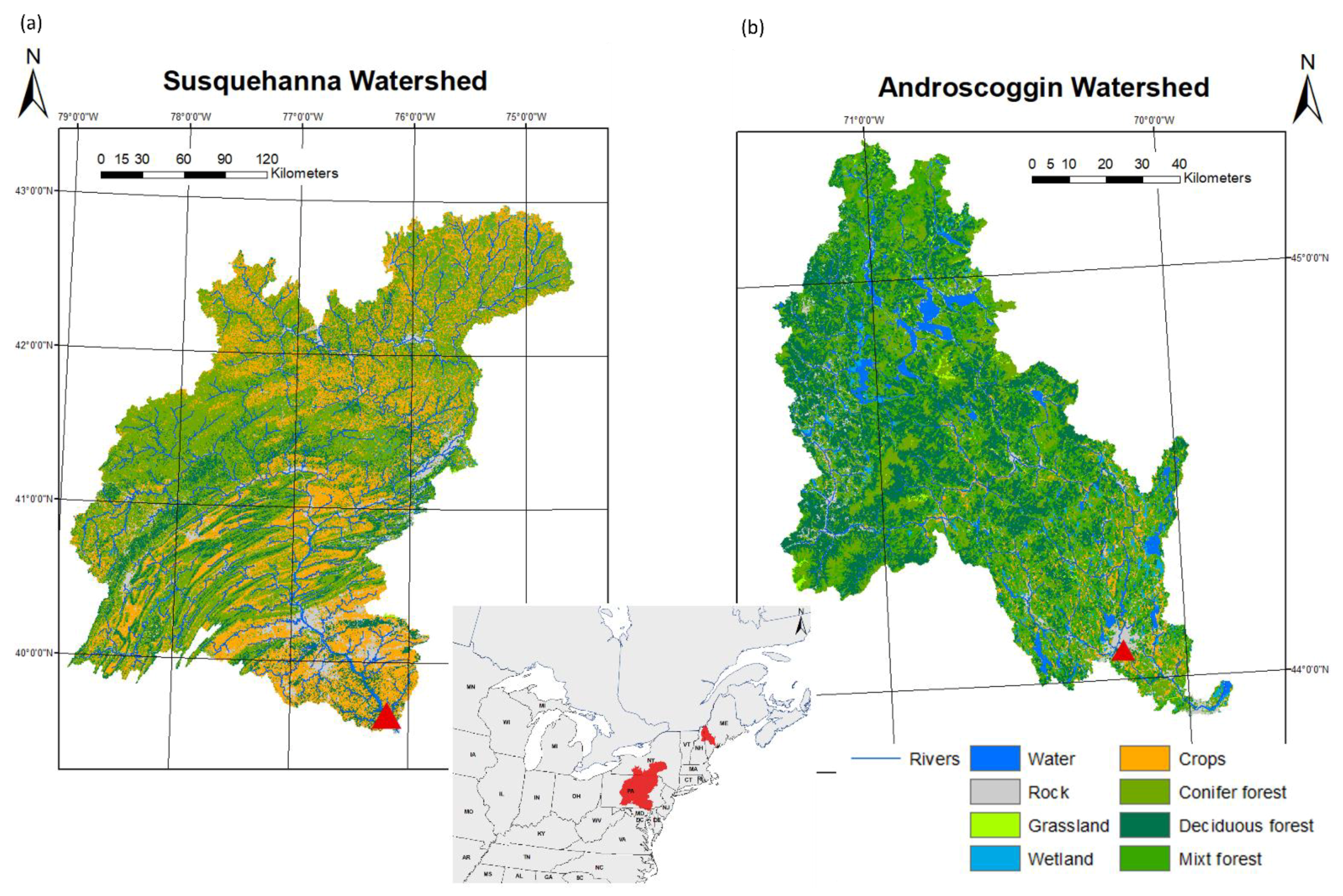
Figure 1.
Land cover of Susquehanna (a) and Androscoggin (b) watersheds. Red triangles indicate the location of the United States Geological Survey (USGS) streamflow stations used (reference number 1,578,310 and 1,059,000 for the Susquehanna and the Androscoggin watersheds respectively).
Figure 1.
Land cover of Susquehanna (a) and Androscoggin (b) watersheds. Red triangles indicate the location of the United States Geological Survey (USGS) streamflow stations used (reference number 1,578,310 and 1,059,000 for the Susquehanna and the Androscoggin watersheds respectively).
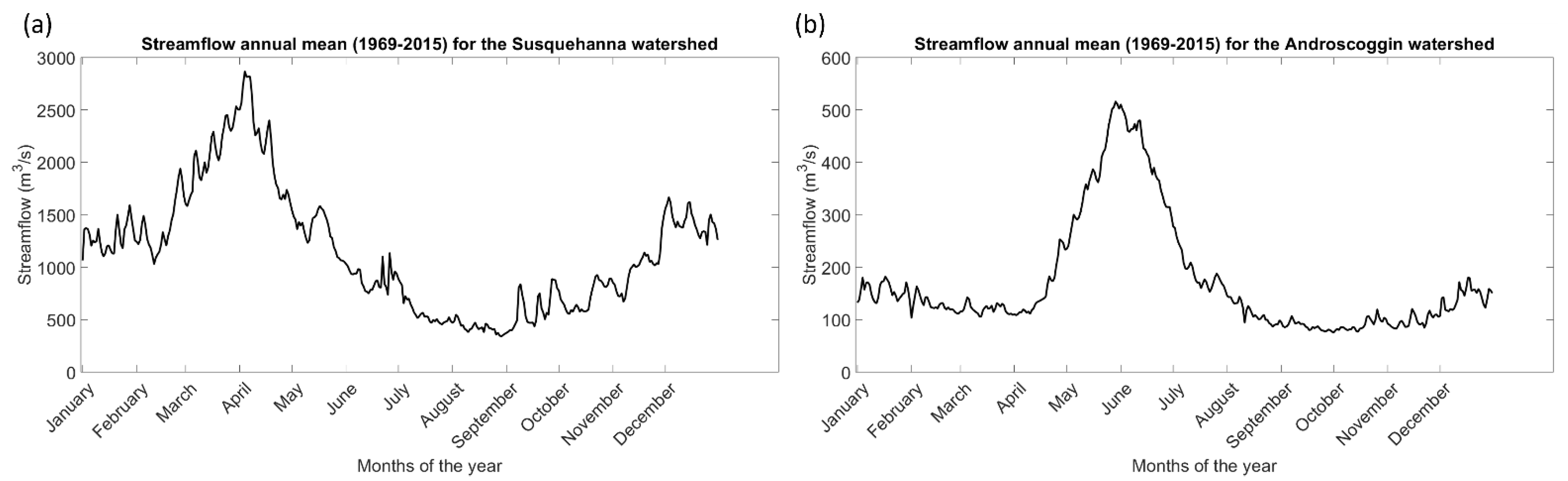
Figure 2.
Mean annual streamflow for (a) Susquehanna and (b) Androscoggin watersheds, generated with datasets covering 47 years (1969–2015).
Figure 2.
Mean annual streamflow for (a) Susquehanna and (b) Androscoggin watersheds, generated with datasets covering 47 years (1969–2015).
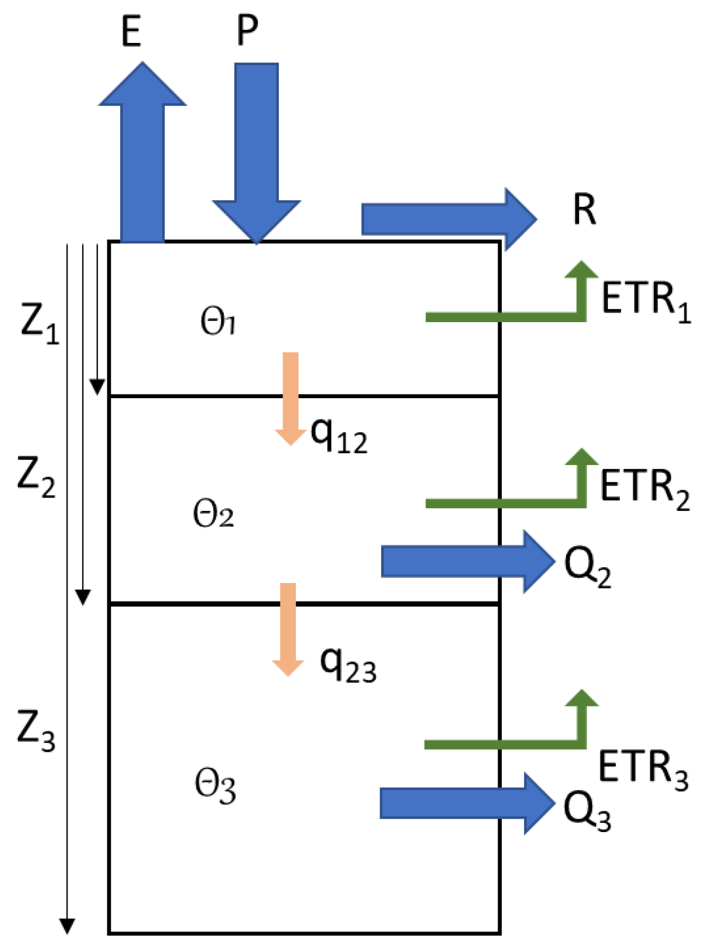
Figure 3.
Schematic representation of BV3C simulation option for vertical water budget in HYDROTEL. The thicknesses of the 3 soil layers are represented by Z1, Z2, and Z3, and the associated soil moisture are Θ1, Θ2, and Θ3, and the relative real evapotranspiration ETR1, ETR2, and ETR3, respectively. Total evaporation, precipitation and surface runoff are designed by E, P, and R, respectively. The interflow and the baseflow are represented by Q2 and Q3, and the baseflow, respectively.
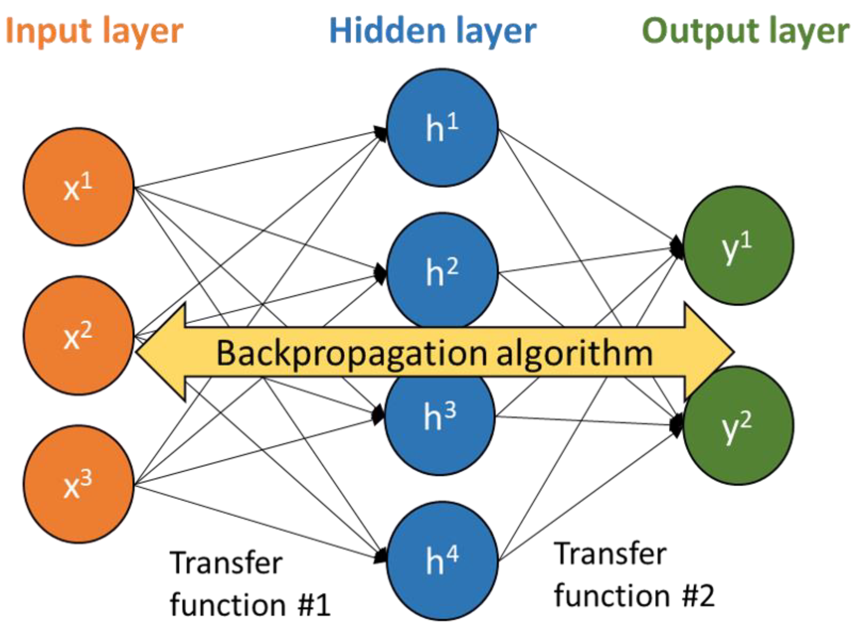
Figure 4.
Schematic representation of a three-layer back-propagated ANN with 3 inputs, 4 hidden neurons, and 2 outputs.
Figure 4.
Schematic representation of a three-layer back-propagated ANN with 3 inputs, 4 hidden neurons, and 2 outputs.
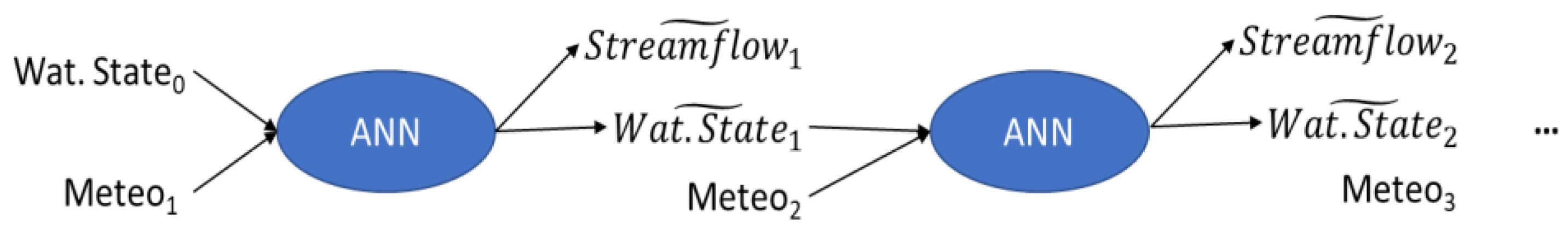
Figure 5.
Schematic representation of the forecast chain used (example for forecasts one and two days in advance and exactly represented 2-SMP and 3-dSMP with update of watershed state variable at each time step). The tilde represents outputs of the ANN model. The index represents the forecast horizon day, with 0 the day of forecasting.
Figure 6.
Evaluation of the number of neurons in the hidden layer for (a) the Androscoggin and (b) the Susquehanna watersheds. Blue boxplots are relative to the training step, while red are for the validation step. Each boxplot is plotted with the 16 summers used in the cross-validation process.
Figure 6.
Evaluation of the number of neurons in the hidden layer for (a) the Androscoggin and (b) the Susquehanna watersheds. Blue boxplots are relative to the training step, while red are for the validation step. Each boxplot is plotted with the 16 summers used in the cross-validation process.
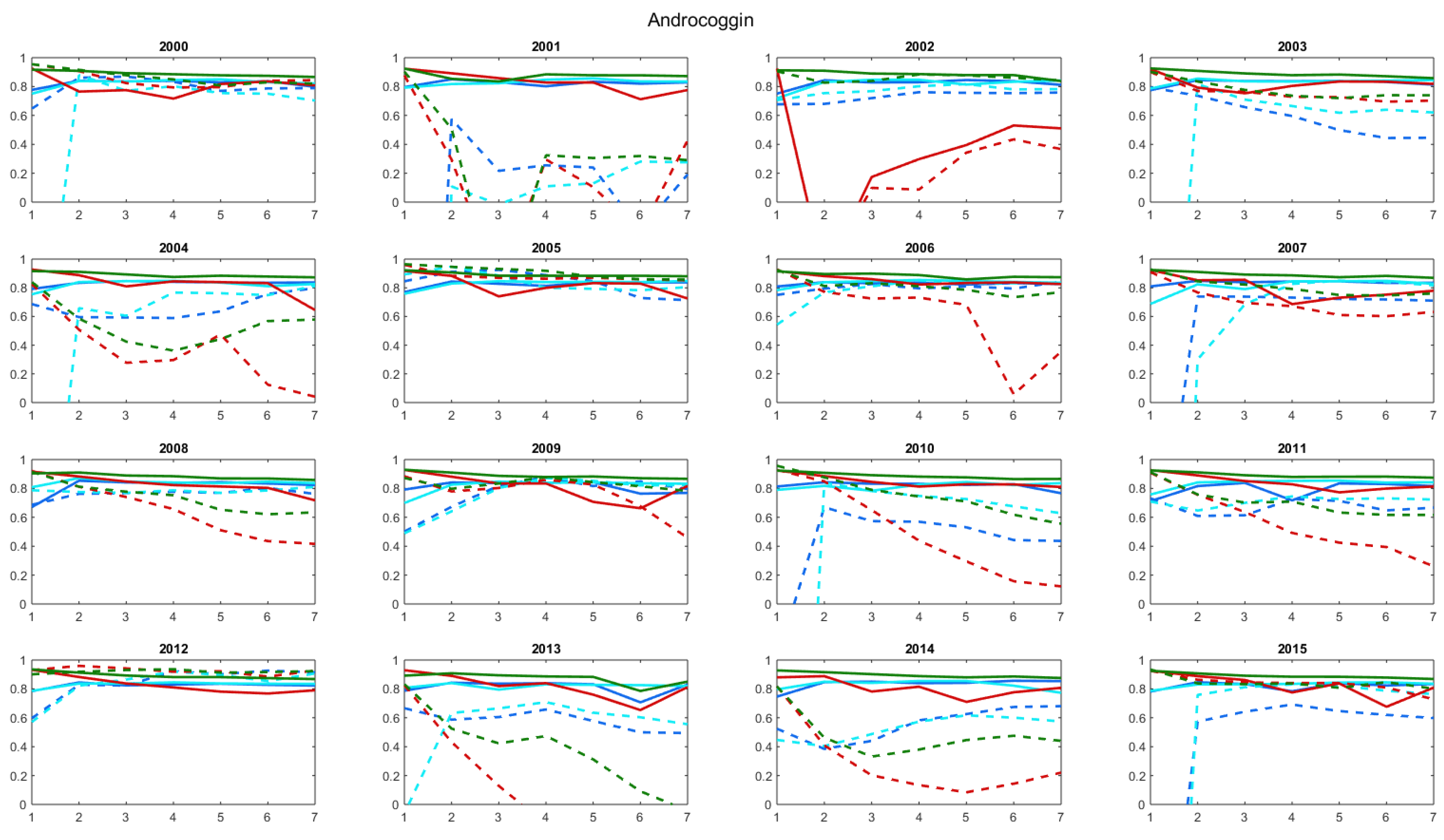
Figure 7.
Evolution of NSE across the 7-day forecast window for the Androscoggin watershed. The training step is in full line, while leave-one-out validation is in dotted line. QP results are represented in red, SMP in blue, dSMP in cyan, and QSMP in green. Each subplot corresponds to a specific step of our cross-validation approach with the year used in validation in sub-title.
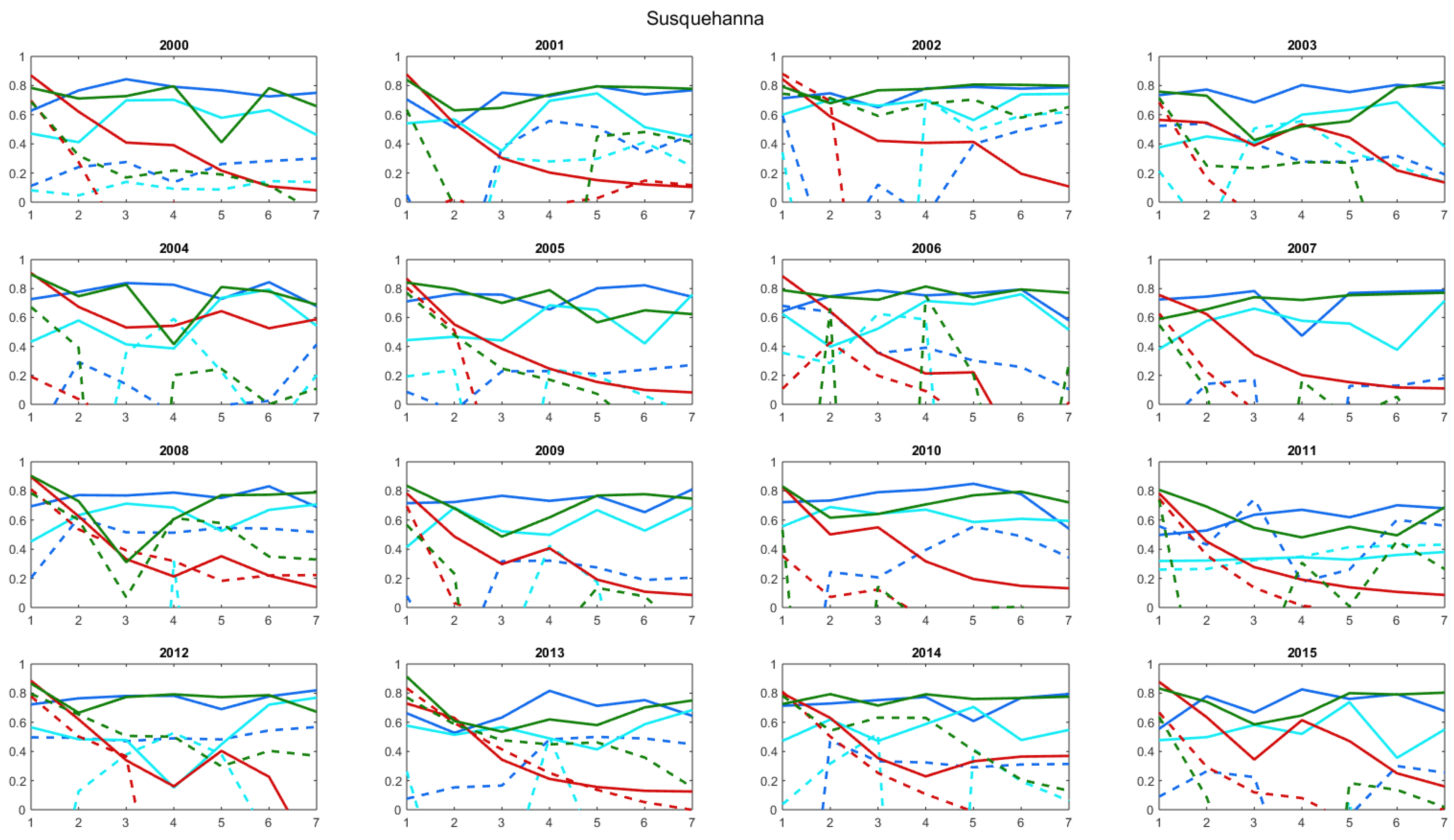
Figure 8.
Evolution of NSE across the 7-day forecast window for the Susquehanna watershed. The training step is in full line, while leave-one-out validation is in dotted line. QP results are represented in red, SMP in blue, dSMP in cyan, and QSMP in green. Each subplot corresponds to a specific step of our cross-validation approach with the year used in validation in sub-title.
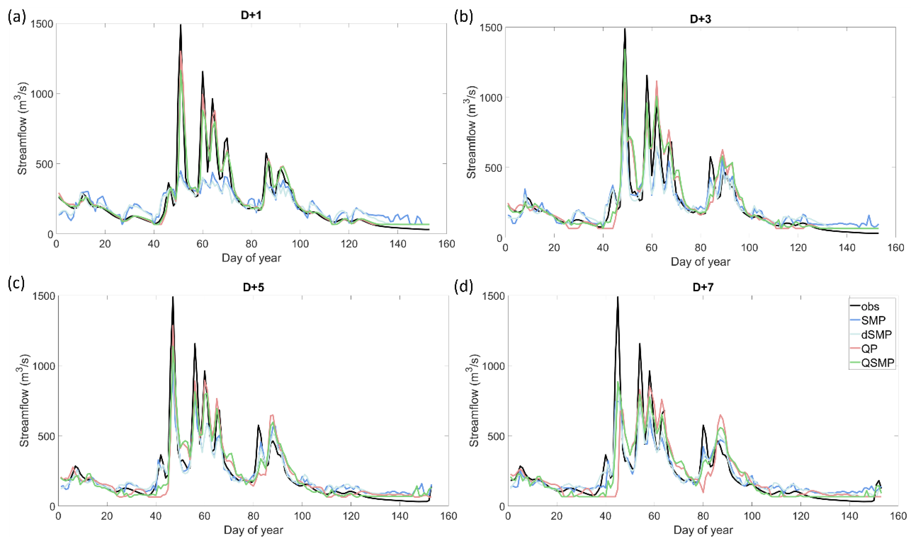
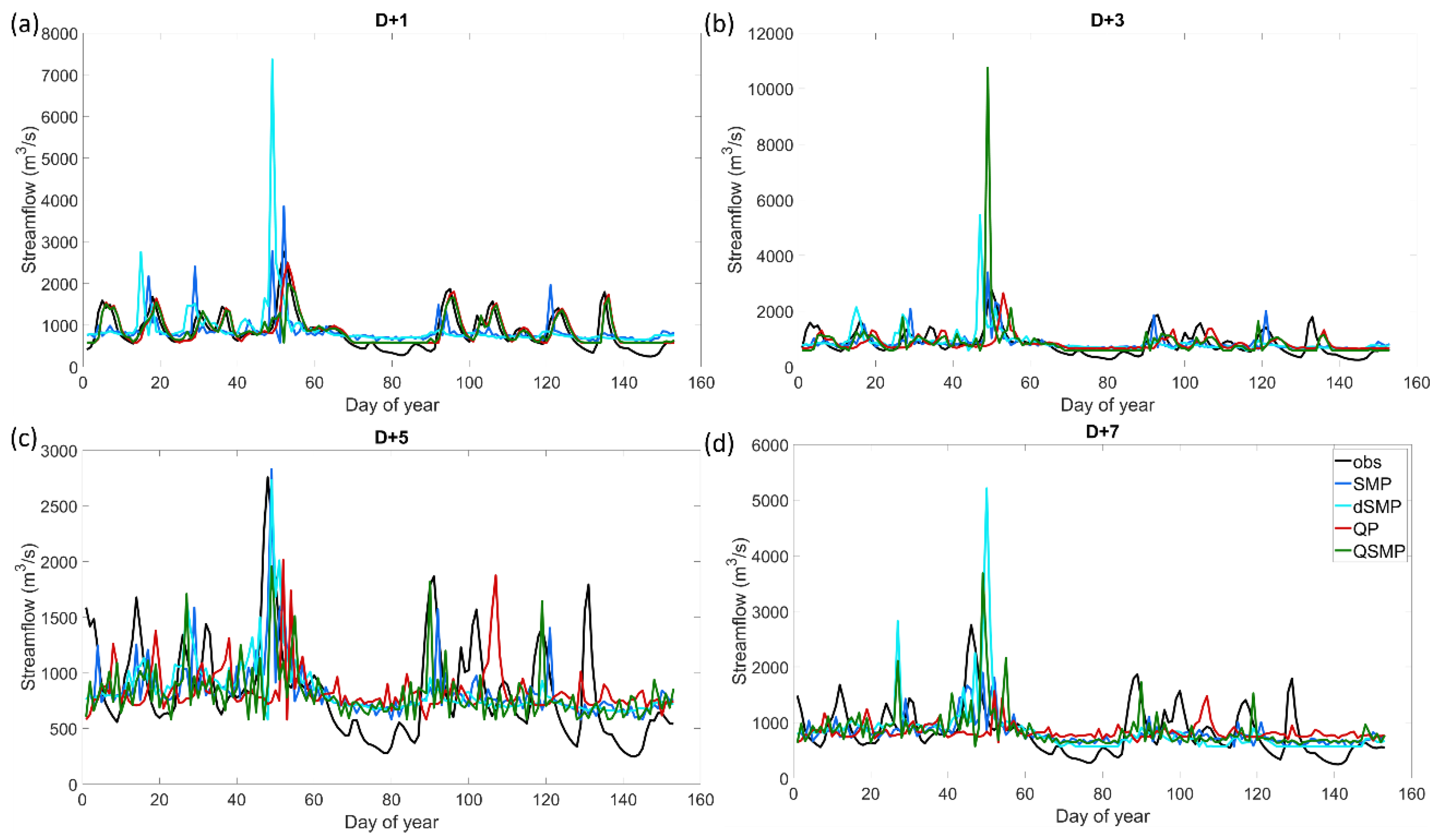
Figure 9.
Hydrographs for the Androscoggin watershed for summer 2009 (validation period) (a) 1, (b) 3, (c) 5 and (d) 7 days in advance.
Figure 9.
Hydrographs for the Androscoggin watershed for summer 2009 (validation period) (a) 1, (b) 3, (c) 5 and (d) 7 days in advance.
Figure 10.
Hydrographs for the Susquehanna watershed for summer 2009 (validation period) (a) 1, (b) 3, (c) 5 and (d) 7 days in advance.
Figure 10.
Hydrographs for the Susquehanna watershed for summer 2009 (validation period) (a) 1, (b) 3, (c) 5 and (d) 7 days in advance.
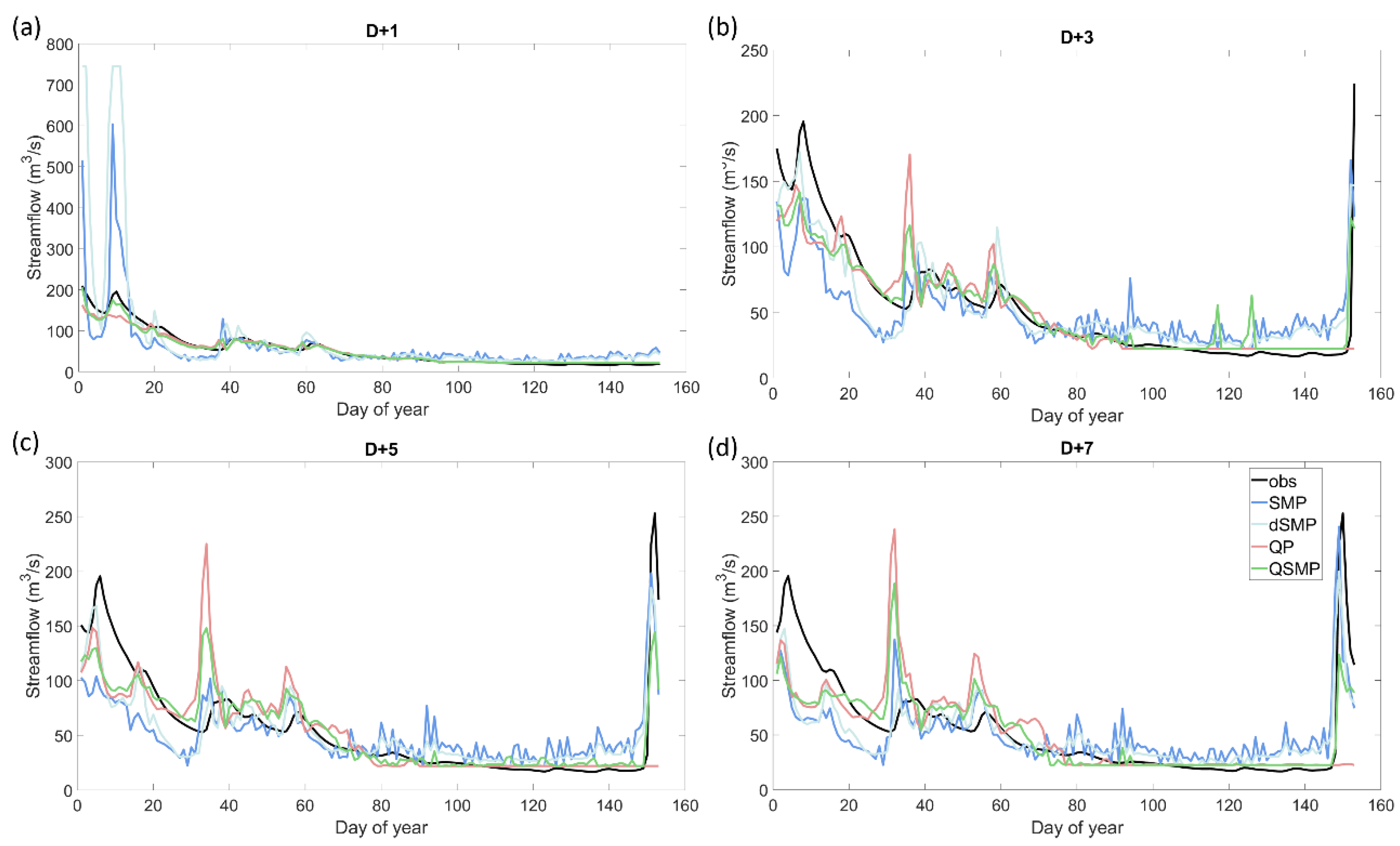
Figure 11.
Hydrographs for the Androscoggin watershed for summer 2010 (validation period) (a) 1, (b) 3, (c) 5 and (d) 7 days in advance.
Figure 11.
Hydrographs for the Androscoggin watershed for summer 2010 (validation period) (a) 1, (b) 3, (c) 5 and (d) 7 days in advance.
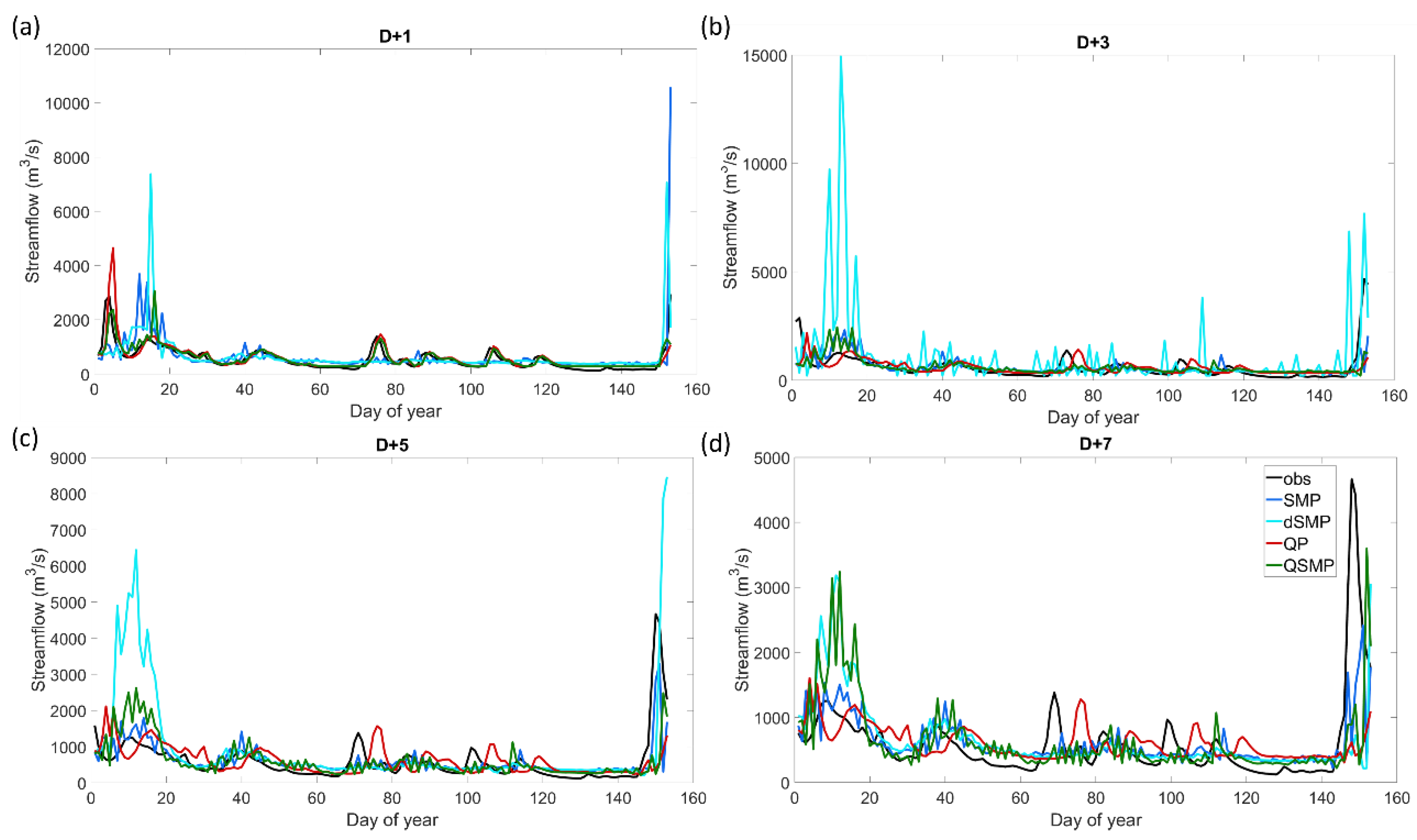
Figure 12.
Hydrographs for the Susquehanna watershed for summer 2010 (validation period) (a) 1, (b) 3, (c) 5 and (d) 7 days in advance.
Figure 12.
Hydrographs for the Susquehanna watershed for summer 2010 (validation period) (a) 1, (b) 3, (c) 5 and (d) 7 days in advance.
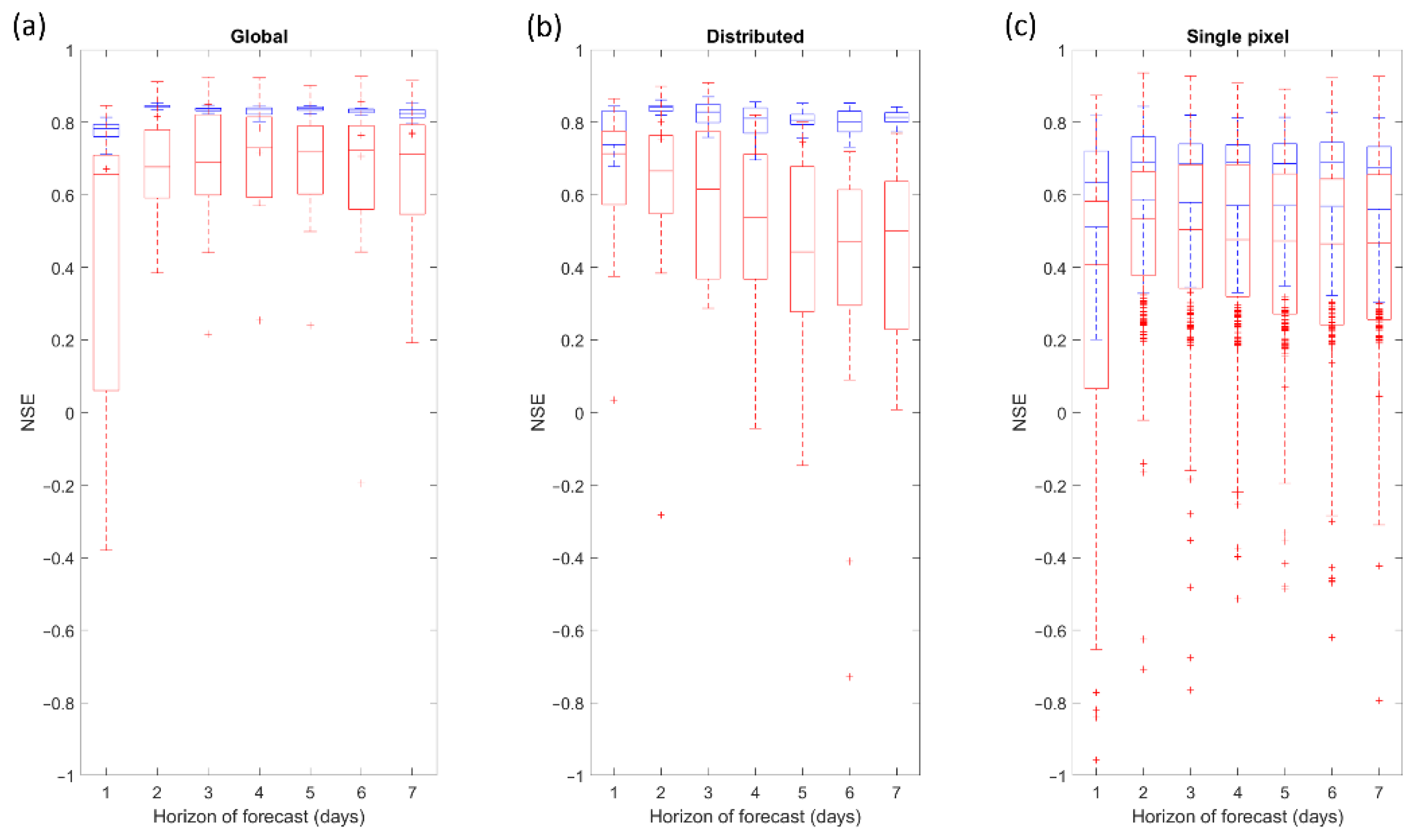
Figure 13.
For the Androscoggin watershed, the evolution of the NSE across the 7-day forecast window for 3 types of input spatialization: (a) global (i.e., grid average), (b) distributed (i.e., full-grid), and (c) single pixel (i.e., each of the 28 grid points individually). Each boxplot represents the dispersion across the 16 years used in cross-validation, blue is training, red is validation.
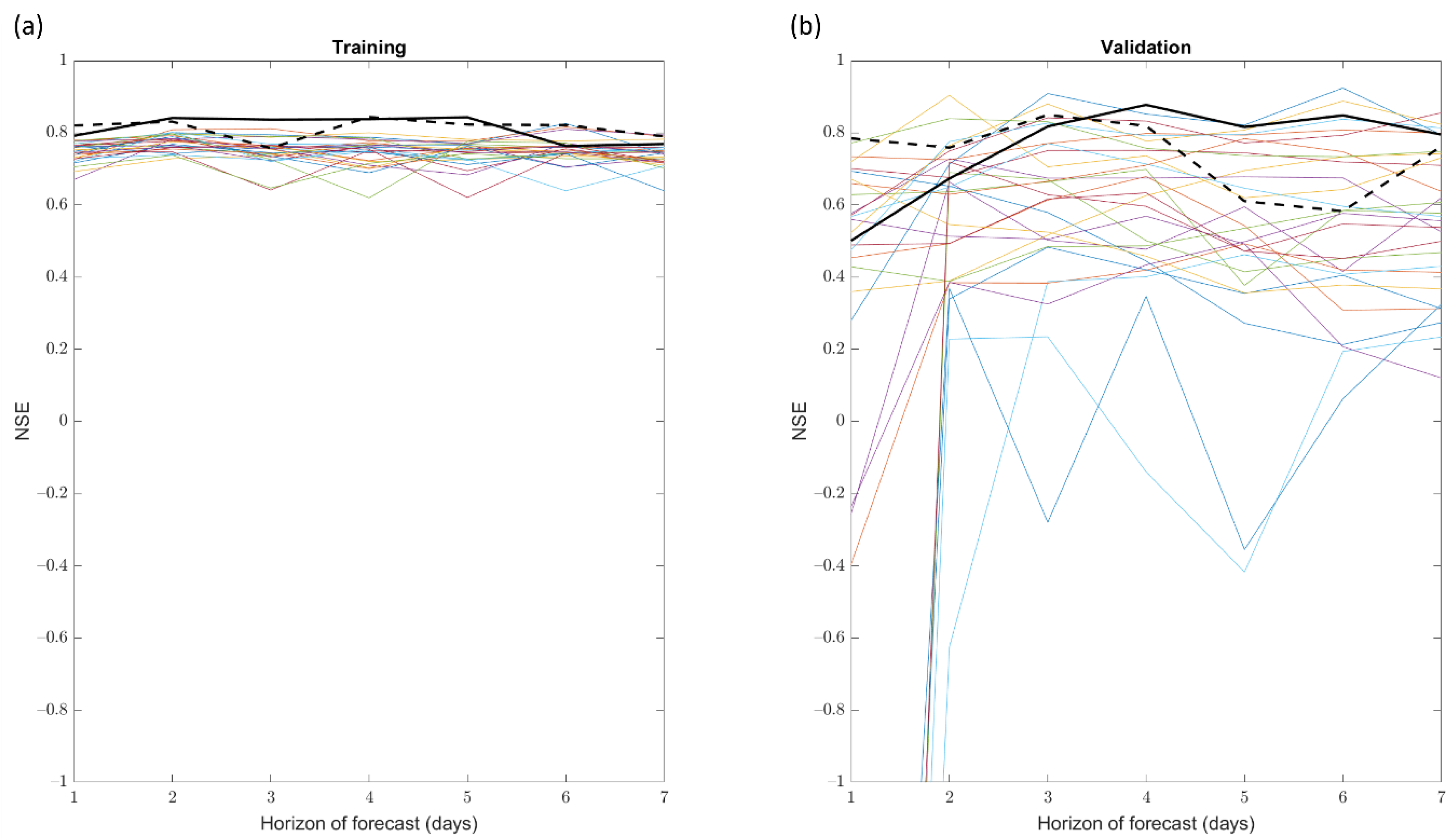
Figure 14.
NSE evolution for the Androscoggin watershed in 2009. (a) Training, (b) Validation. Colored lines for each pixel, dotted line for the distributed model, and full line for the global one.
Figure 14.
NSE evolution for the Androscoggin watershed in 2009. (a) Training, (b) Validation. Colored lines for each pixel, dotted line for the distributed model, and full line for the global one.
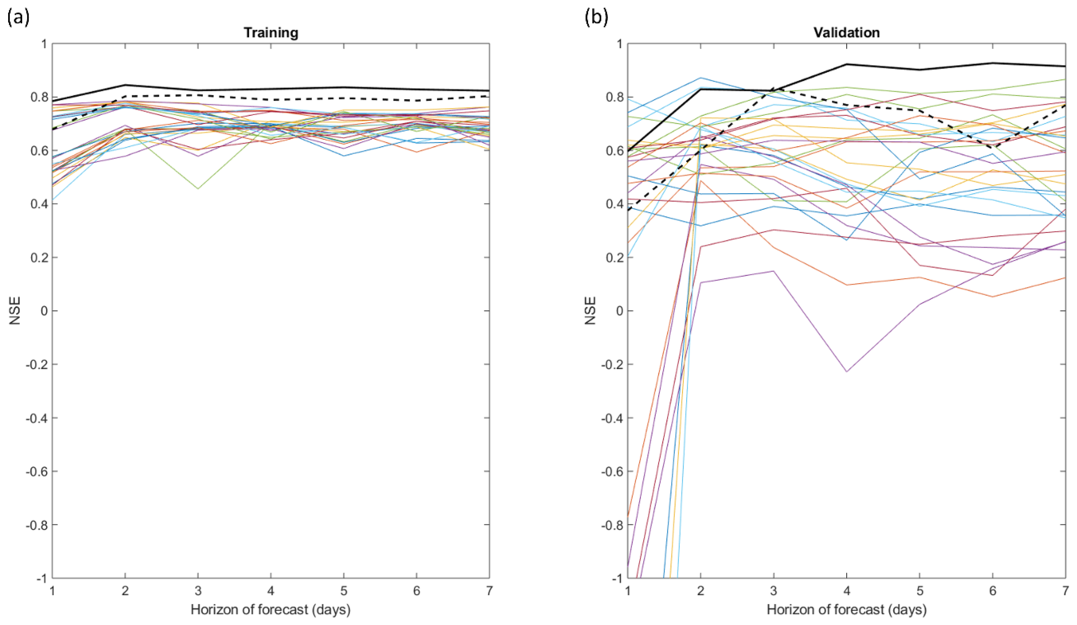
Figure 15.
NSE evolution for Androscoggin watershed in 2012. (a) Training, (b) Validation. Colored lines for each pixel, dotted line for the distributed model, and full line for the global one.
Figure 15.
NSE evolution for Androscoggin watershed in 2012. (a) Training, (b) Validation. Colored lines for each pixel, dotted line for the distributed model, and full line for the global one.
Table 1.
Return streamflow for four specific return periods: 2, 10, 25, and 100 years for the two watersheds, generated with datasets covering 47 years (1969–2015).
Table 1.
Return streamflow for four specific return periods: 2, 10, 25, and 100 years for the two watersheds, generated with datasets covering 47 years (1969–2015).
| Watershed | Q2 (m3/s) | Q10 (m3/s) | Q25 (m3/s) | Q100 (m3/s) |
|---|
| Androscoggin | 161 | 424 | 556 | 751 |
| Susquehanna | 939 | 2772 | 3695 | 5059 |
Table 2.
Summary of HYDROTEL’s defined sub-models and associated simulation options. Simulation options used in this study to generate hydrometeorological ‘observations’ are bolded.
Table 2.
Summary of HYDROTEL’s defined sub-models and associated simulation options. Simulation options used in this study to generate hydrometeorological ‘observations’ are bolded.
| Sub-Models | Simulation Options |
|---|
| Interpolation of precipitation | Thiessen polygon |
| | Weighted mean of nearest 3 stations |
| Snowmelt | Modified Degree-day |
| Evapotranspiration | Thornthwaite |
| | Linacre |
| | Penman |
| | Priestley-Taylor |
| | Hydro-Québec |
| Vertical water budget | CEQUEAU |
| | Three-Layer Vertical Budget (BV3C) |
| Surface and subsurface runoff | Kinematic wave equation |
| Channel routing | Modified kinematic wave equation |
| | Diffusive wave equation |
Table 3.
Combinations of variables defined as artificial neural network (ANN) inputs.
Table 3.
Combinations of variables defined as artificial neural network (ANN) inputs.
| No. and Name | Watershed State Variables | Meteorological Variables |
|---|
| | At Day D-1 | At Day D and Day D-1 |
|---|
| 1—QP | Downstream Streamflow | Precipitation |
| 2—SMP | Surface Soil Moisture | Precipitation |
| 3—dSMP | Deep Soil Moisture | Precipitation |
| 4—QSMP | Downstream Streamflow | Precipitation |
| | Surface Soil Moisture | |
Table 4.
Number of inputs for the ANN model depending on the combination of variables and the spatial distribution. With a regular grid, information is only given for the Androscoggin watershed (An.).
Table 4.
Number of inputs for the ANN model depending on the combination of variables and the spatial distribution. With a regular grid, information is only given for the Androscoggin watershed (An.).
| No. and Name | Average | Regular Grid |
|---|
| 1—SMP | | |
| 2—dSMP | 3 | 84 (An.) |
| 3—QP | | |
| 4—QSMP | 4 | 112 (An.) |
Table 5.
Nash–Sutcliffe efficiency (NSE) values for Susquehanna and Androscoggin for summer 2009, a relatively wet year, as validation period.
Table 5.
Nash–Sutcliffe efficiency (NSE) values for Susquehanna and Androscoggin for summer 2009, a relatively wet year, as validation period.
| Watershed | Susquehanna | Androscoggin |
|---|
| Forecast Horizon | D + 1 | D + 3 | D + 5 | D + 7 | D + 1 | D + 3 | D + 5 | D + 7 |
|---|
| 1-QP | train. | 0.784 | 0.298 | 0.192 | 0.086 | 0.928 | 0.835 | 0.707 | 0.818 |
| valid. | 0.696 | −0.057 | −0.328 | −0.116 | 0.884 | 0.803 | 0.827 | 0.458 |
| 2-SMP | train. | 0.716 | 0.767 | 0.765 | 0.812 | 0.792 | 0.837 | 0.843 | 0.769 |
| valid. | 0.080 | 0.318 | 0.274 | 0.205 | 0.501 | 0.818 | 0.816 | 0.796 |
| 3-dSMP | train. | 0.415 | 0.523 | 0.669 | 0.685 | 0.699 | 0.847 | 0.842 | 0.833 |
| valid. | −1.321 | −0.369 | 0.175 | −0.603 | 0.489 | 0.803 | 0.852 | 0.824 |
| 4-QSMP | train. | 0.835 | 0.486 | 0.768 | 0.747 | 0.930 | 0.887 | 0.883 | 0.867 |
| valid. | 0.567 | −2.163 | 0.135 | −0.215 | 0.873 | 0.834 | 0.844 | 0.783 |
Table 6.
NSE values for Susquehanna and Androscoggin for summer 2010, a relatively dry year as validation period.
Table 6.
NSE values for Susquehanna and Androscoggin for summer 2010, a relatively dry year as validation period.
| Watershed | Susquehanna | Androscoggin |
|---|
| Forecast Horizon | D + 1 | D + 3 | D + 5 | D + 7 | D + 1 | D + 3 | D + 5 | D + 7 |
|---|
| 1-QP | train. | 0.828 | 0.550 | 0.195 | 0.132 | 0.924 | 0.846 | 0.829 | 0.810 |
| valid. | 0.355 | 0.123 | −0.114 | −0.061 | 0.928 | 0.650 | 0.295 | 0.122 |
| 2-SMP | train. | 0.723 | 0.791 | 0.849 | 0.541 | 0.814 | 0.833 | 0.824 | 0.767 |
| valid. | −1.914 | 0.207 | 0.555 | 0.344 | −0.380 | 0.574 | 0.531 | 0.436 |
| 3-dSMP | train. | 0.556 | 0.643 | 0.586 | 0.595 | 0.790 | 0.784 | 0.844 | 0.837 |
| valid. | −2.189 | −7.368 | −2.631 | −0.261 | −5.375 | 0.782 | 0.727 | 0.628 |
| 4-QSMP | train. | 0.831 | 0.642 | 0.770 | 0.721 | 0.824 | 0.892 | 0.877 | 0.866 |
| valid. | 0.534 | 0.143 | −0.002 | −0.078 | 0.957 | 0.790 | 0.710 | 0.555 |


