Statistical Evaluation of the Influences of Precipitation and River Level Fluctuations on Groundwater in Yoshino River Basin, Japan

Abstract

Precise evaluation of the correlations among precipitation, groundwater and river water enhance our understanding on regional hydrological circulation and water resource management. The innovative and efficient use of wavelet analysis has been able to identify significant interactions in the spatial and temporal domains and to estimate the recharge travel time. In this paper, a wavelet analysis was utilized to analyse 43 years of monthly, and 2 years of daily, precipitation, river level and groundwater level data in the Yoshino River Basin, Japan. There were two main results: (1) There was a significant influence of precipitation and river on groundwater, with a periodicity of 4–128 days, 1 year and 2–7 years. The periodicity of 1 year was correlated with seasonal variability. The significant interaction at 4–128 days mainly occurred in the rainy season. The 2–7-year oscillation of aquifer water levels was determined by precipitation. (2) The recharge-water travel times in the study area estimated from the arrow patterns in the precipitation–groundwater wavelet coherence (WTC) were consistent for each observation well. The response times of the aquifer to precipitation were 1 day and 3–6 days in 2013 and 2014, respectively. The different time lags were likely determined by the timing of maximum daily precipitation.

1. Introduction

As the largest distributed storage of fresh water, groundwater plays an critical role in sustaining ecosystems and facilitating human adaptation to climate change [1]. Water level monitoring in aquifers constitutes the principal means of tracking changes in groundwater storage over time, which provides information regarding the availability of renewable groundwater resources. Temporal groundwater level changes of piezometric levels typically occurs at two distinct time scales: long term (interannual and seasonal variability) and short term (daily or subdaily fluctuations) [2]. The interannual variability of hydrological processes is commonly discussed with regard to large-scale climatic phenomenon, such as solar activity, the El Niño Southern Oscillation (ENSO) and the North Atlantic Oscillation (NAO), while seasonal fluctuations are widely considered to be related to local climatic indices, such as precipitation, temperature, air pressure and humidity. An analysis of aquifer responses to the possible influencing factors could improve our understanding of the regional water circulation and therefore guide water resource management [3].

Climate change has been shown to have direct and indirect influences on subsurface hydrological processes [1,4]. The impacts of large-scale climatic phenomena on subsurface hydrological patterns commonly occur at the decadal and annual scale [3]. Solar activity and climatic anomalies affect the planetary-scale atmospheric circulation in a frequency-dependent manner, which alters regional precipitation characteristics [5]. Precipitation events affect aquifer water levels by changing the recharge patterns [3,6]. Although piezometric levels are commonly influenced by climatic indices, fluctuations in piezometric levels are also driven by various hydrological processes at different spatial and temporal scales. Natural external stresses (air pressure changes, tidal or river water level fluctuations, earth tides, tectonic events) can affect fluctuations in aquifer water level. Dynamic interactions between groundwater and seawater/surface water commonly occur in aquifers where hydraulic connections exist [2,7,8]. The direct, rapid responses of aquifers to external hydraulic stresses serve as an effective tracer to depict hydrological processes. However, the lack of detailed groundwater observations limits our understanding of the interactions between precipitation, external hydrological processes and aquifers, especially over varying temporal scales.

Most previous studies employed spectral analysis to identify the aquifer responses to possible influent factors, such as precipitation variability [9], tidal effects [10,11] and lake level fluctuations [12]. A spectral analysis can be used to evaluate the coherence and phase lag between external hydrological processes and groundwater-level responses in the frequency domains, and to estimate the degree of influence and travel time of external stresses to aquifers. However, a spectral analysis only determines the frequency content of aquifer water levels. Temporal variation in the groundwater-level response to influent factors can be evaluated using a wavelet analysis [13]. The impact of climate and anthropic effects on aquifers has been studied using a wavelet analysis in many parts of the world [3,6,14]. The wavelet analysis can not only evaluate the variability of the aquifer in different spatial and temporal frequencies using the signal amplification function, but also analyse the interaction between possible factors and groundwater using coherence and cross-spectrum functions. The aquifer’s teleconnection with climate indices (ENSO index, NAO index et al.), the interaction with local climate variations (precipitation, air temperature, barometric pressure et al.), and the responses to external stresses (tidal effect, pumping et al.) can be assessed based on wavelet techniques. Additionally, the impact of climate and anthropic pressures on groundwater resources can be evaluated to improve our understanding of water resource management. However, the systematic analyses on the interaction between precipitation, rivers and groundwater from short-term to long-term timescales have not been assessed.

The objectives of this study were: (1) to identify the interannual and interdecadal variability of shallow groundwater level fluctuations and the related hydrological processes (precipitation and river level) in the Yoshino River Basin, Japan, at different spatial and temporal scales; and (2) to interpret the interactions between precipitation, river levels and groundwater by analysing coherence and phase lag based on a wavelet technique. Evaluation and quantification of the variability of hydrological processes and their responses to related influencing factors provide guidance on regional water resource management.

2. Study Area and Methodology

2.1. Study Area and Datum

The study area is located in the lower Yoshino catchment in south Japan (Figure 1). The Yoshino River is 194 km in length and has a watershed of 3750 km². The study area is a watershed with an area of about 840 km² located in Tokushima Plain. The plain consists of alluvial delta clay and sand, and about 75% of the study area is covered by forests and meadow. The elevation of the investigated watershed decreases from west to east and ranges from −10 to 185 m. Pacific climate patterns dominate in the study area. The mean annual precipitation from 1892 to 2014 at the Tokushima meteorological station was about 1650 mm per year, and the average annual air temperature from 1890 to 2014 was about 15.5 °C. A national meteorological station, hydrological station and four observation wells are located along the Yoshino River. The Ikeda Dam is located about 48 km upstream of the hydrological station, and the Daiju-Zeki Weir Dam is located about 11 km downstream of the station. These two large dams were constructed mainly for domestic and agricultural water usages, and the natural river regimes were consequently altered by dam regulation and artificial water intake. However, this manuscript emphasizes the influence of river level fluctuation on the aquifer in the study area, and the river–aquifer interaction in spatial and temporal domains can be interpreted properly even if the time series of river water levels is influenced artificially.

The data used in the analysis of precipitation, piezometric levels and river levels consist of 43 years (from 1972 to 2014) of daily data. Daily precipitation was recorded by an automatic rain gauge installed at the Tokushima meteorological station. The groundwater level (with reference to the annual mean sea level in Tokyo Bay) was observed using pressure water level gauges installed in the observation wells. The study aquifer is composed of silt, sand and gravel. The screens of the observation wells were positioned at depths from 2 to 10 m, and therefore the study considered the groundwater present in the unconfined aquifer in the study area. The transmissivity of the unconfined aquifer is investigated and calculated as about 1000 m²/day in the study area. No artificial exploitation was detected in the study area, and the aquifer water levels were inferred to be disturbed slightly by human activity. No dams or water diversions were built in the upper reaches. The river level was measured by a bubble-type water gauge installed in the hydrological station, and no artificial channels were found in the station.

A time series of precipitation and aquifer water levels in observation wells 1 to 4 and the river level are presented in Figure 2a–f, respectively. Figure 2 shows that the daily precipitation, piezometric levels and river levels fluctuated periodically. Figure 2c shows the aquifer water levels in well 2 suddenly changed in 2004, which was associated with a shift in the measurement location, and the aquifer water levels after 2004 were adjusted for consistence. There were several water level measurements missing during 1976 and 1978 for well 4. An interpolation process was used to resolve this problem in the subsequent analysis. The time series were standardized before subsequent analyses.

2.2. Data Analyses Methods

The multiresolution analysis and continuous wavelet analysis approaches were applied in this study. First, wavelet decomposition was implemented to extract aquifer water levels and their possible impact factors across different resolution levels, and the standard deviations (SD) were calculated to quantify the multiresolution levels. Then, a cross-correlation between aquifer water levels and potential impact variables across different levels was conducted to reveal the dependence of aquifer water level on the possible influencing factors. Finally, a wavelet analysis was performed to quantify the temporal features in different periods of precipitation, and aquifer and river levels. A wavelet coherence (WTC) analysis was applied to detect the aquifer responses to precipitation and river levels in both the time and frequency domains.

A multiresolution analysis can be applied to decompose a time series into a series of successive approximations and details in increasing order of resolution to study signals at different resolutions [14]. Wavelet decomposition returns the wavelet coefficients of the signal at different levels through the implementation of specific wavelets. Wavelet decomposition is performed based on designed signal filters [3]. The details of the algorithm can be found in the paper by Mallat [15].

To quantify the relationship between two signals at different resolution levels, a multiresolution cross-analysis [14] was applied. Cross-correlation evaluates the similarity of two time series as a function of the lag of one series in relation to the other. The cross-correlation function (CCF) analysis was applied to identify the influence of possible factors on aquifer water levels in different frequency domains. The calculation of the CCF is described by Charlier [14].

A wavelet analysis assesses the variation in a signal in both the temporal and frequency domains [13]. In the field of hydrology, this technique is applied in two aspects: to determine the spatial and temporal variation of hydrological factors, including precipitation, river discharge and aquifer water levels [16,17,18,19]; and to quantify the interaction between hydrological variations and climatic indices, such as solar activity [11,20], the North Atlantic Oscillation [6,21], and the ENSO [20,22].

The wavelet techniques utilized in this study included the wavelet power spectrum (WPS) and WTC. The WPS represents the magnitude of the variance in a time series at a given frequency and location in time. This technique provides an effective approach to analyse the variability of hydrological processes. The WPS [23] is defined as the square absolute value (or square amplitude) of the wavelet transform coefficients.

To eliminate the distortion of a wavelet analysis in time–frequency domains, the concept of the cone of influence (COI) was introduced, in which the e-folding time function is used to overcome edge effects [23]. The edge effects are negligible for wavelet spectra located in the COI region. The statistical significance of wavelet power can be assessed relative to the null hypothesis that the signal is generated by a stationary process with a given background power spectrum. A significance test was conducted using the Monte Carlo method [23] and a 5% significance level was adopted. The WPS enables us to characterise the degree of complexity of a simplex signal. To assess the relationship between two signals in the time–frequency domains, a cross-wavelet analysis should be introduced [13]. The WTC can determine a significant coherence even though the common power is low [24]. Concerning hydrological issues, this approach has been used to access the influence of ENSO on stream flow [22], construct models to forecast river flow [25] and evaluate timing errors in hydrological predictions [26].

The significance contour for the cross-wavelet analysis can be found using the chi-squared distribution, with details of the algorithm provided by Torrence and Compo [23]. The 5% significance level was considered in this paper. The details of the involved wavelet techniques in this study are described in the relevant references [17,23,24]. All subsequent computations and analyses were conducted within the MATLAB environment.

3. Results

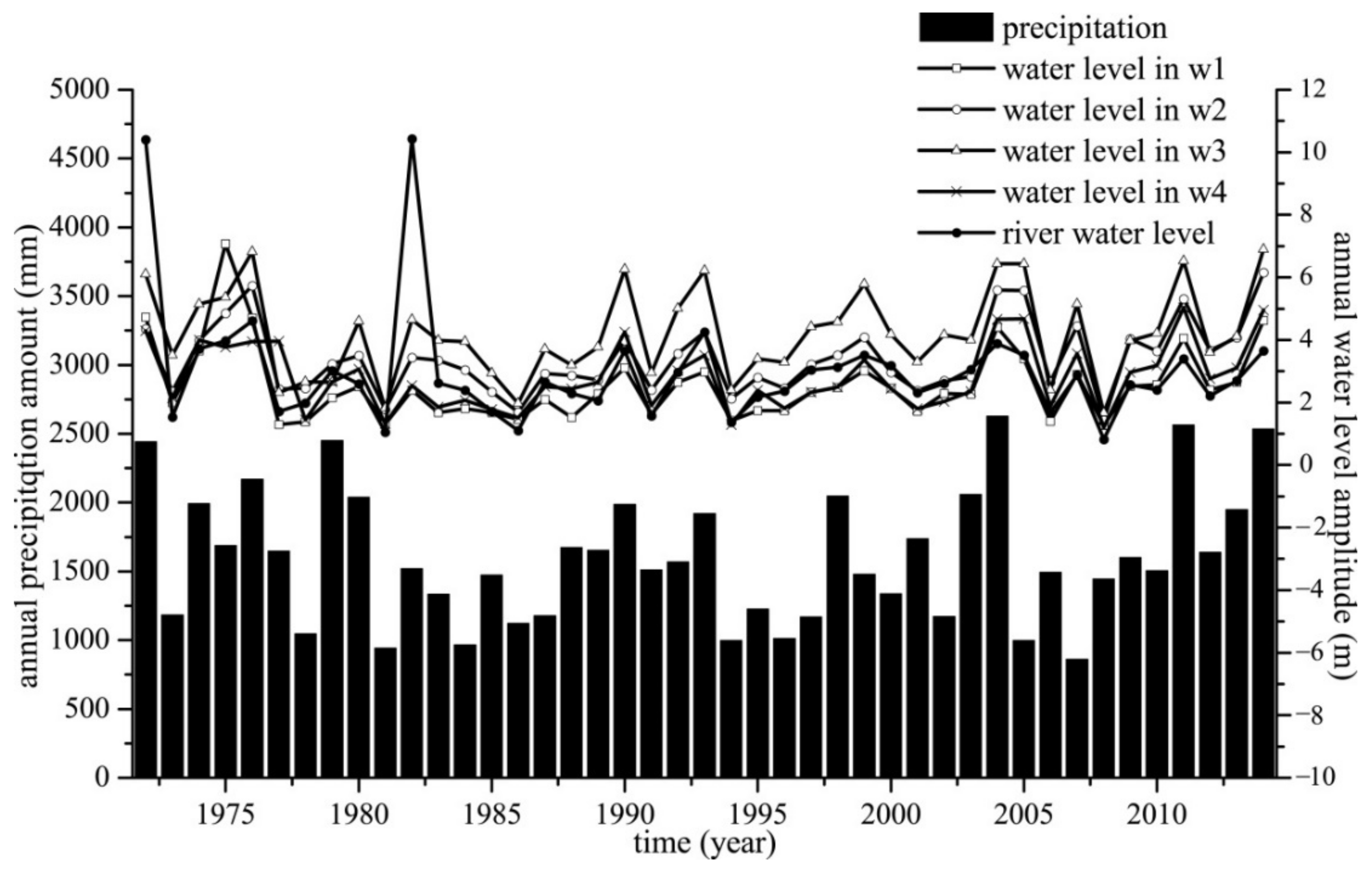
3.1. Variability of Hydrological Time Series

To interpret the characteristics of hydrological variability in the study area, the mean, maximum, minimum, variance and average annual amplitude of hydrological variables were calculated (

Table 1. Standard deviation of the standardized hydrological signals by multiresolution levels (from level 1 to level 12).

Level	Aquifer Water Level				Precipitation	River Level	Barometric Pressure	Humidity	Air Temperature	Sunspot Number	SST
	No. 1	No. 2	No. 3	No. 4
1	0.087	0.095	0.139	0.124	0.616	0.258	0.272	0.434	0.094	0.071	0.026
2	0.123	0.144	0.199	0.140	0.510	0.322	0.410	0.481	0.126	0.097	0.030
3	0.155	0.169	0.238	0.141	0.398	0.331	0.373	0.383	0.130	0.172	0.042
4	0.192	0.183	0.284	0.169	0.299	0.333	0.271	0.283	0.107	0.310	0.063
5	0.215	0.180	0.279	0.178	0.212	0.300	0.227	0.228	0.084	0.212	0.070
6	0.221	0.162	0.268	0.188	0.153	0.267	0.148	0.200	0.081	0.157	0.103
7	0.228	0.141	0.280	0.205	0.112	0.213	0.158	0.165	0.092	0.155	0.180
8	0.446	0.221	0.554	0.401	0.150	0.357	0.662	0.460	0.953	0.124	0.261
9	0.227	0.094	0.193	0.166	0.072	0.263	0.067	0.077	0.096	0.104	0.557
10	0.309	0.114	0.158	0.177	0.036	0.260	0.052	0.061	0.092	0.152	0.621
11	0.277	0.119	0.114	0.151	0.029	0.246	0.062	0.078	0.087	0.547	0.284
12	0.267	0.184	0.143	0.219	0.031	0.157	0.072	0.041	0.105	0.497	0.191

). In a hydrological year in Japan, the maximum river and aquifer water level always occurred in May or June, and the minimum always occurred in December or January; this pattern was associated with the local precipitation. The daily mean, maximum and minimum precipitation amounts from 1972 to 2014 were 4.4, 429.50 and 0.10 mm, respectively. The mean, maximum and minimum water levels in wells 1 and 2 were much higher than those of the other wells and the river. There were no significant differences in the average annual amplitude between the aquifer and river levels.

For a better visualization of the annual fluctuation of hydrological variables, the annual amplitudes of aquifer and river levels were calculated and are shown in Figure 3. It was observed that the changing water level amplitudes in the aquifer and river were closely matched. The annual amplitude of the aquifer water level was always higher than the corresponding amplitude of the river level. The annual precipitation amount was also used to investigate the relationships among precipitation, aquifer level and river level. High annual amplitudes of aquifer and river levels were observed in association with high precipitation amounts, while most of the low amplitudes were associated with the low precipitation amounts.

Wavelet decomposition was used to visualize the spatial distribution of hydrogeological energy in different resolution levels. Multiresolution at 10 levels was performed on the data, and the multiresolution analysis results for precipitation, river levels and aquifer water levels (well 1 is used an example) are shown in Figure 4. The high energy of precipitation was mainly concentrated in the high-frequency domain (corresponding to 1–8 days), indicating that precipitation events lasting several days explained most of the variance in the precipitation signal. Both the river and aquifer water levels had high energy at all levels. From levels 1 to 7, we observed a high energy distribution in the bands of 1972 to 1985 and 1990 to 2005 for river levels. The high energy in aquifer water levels mainly occurred in the bands of 1972 to 1975 and 1990 to 2005 at levels 1 to 7.

To quantify the energy across different multiresolution levels, the SD was calculated for each standardized time series (Table 1). As described previously, the SD of aquifer water levels and river levels had an insignificant peak at level 8, indicating high energy at all levels. Table 1 shows that the SD of precipitation decreased from 0.616 to 0.036 for low-to-high multiresolution levels, indicating that the high energy was concentrated in the high-frequency domain.

3.2. Correlations of Hydrological Processes

To access the dependence of groundwater level on possible climatic and hydrological variables in the study area, the correlation coefficients between possible impact factors and aquifer water levels were calculated and shown in

Table 2. Correlation coefficients between possible impact factors and aquifer water levels.

	Precipitation	River Level	Barometric Pressure	Humidity	Air Temperature	Sunspot Number	SST
w1	0.234	0.434	−0.257	0.286	0.349	0.010	−0.059
w2	0.188	0.391	−0.120	0.218	0.129	0.270	0.010
w3	0.339	0.640	−0.367	0.398	0.471	0.119	−0.101
w4	0.221	0.445	−0.268	0.261	0.357	−0.160	−0.155
average	0.246	0.478	−0.253	0.291	0.327	0.059	−0.076

. The results show that the groundwater level in the study area shows relatively high negative correlations (absolute value above 0.24) with the barometric pressure and positive correlations (absolute value above 0.24) with precipitation, river level, humidity and air temperature. However, the high correlation with the humidity and air temperature might be explained by the synchronous seasonal variation feature instead of interaction. Relative low correlations were detected between aquifer water levels and sunspot number, SST, indicating the solar activity and ENSO have weak influence on the aquifer in the study area.

To identify the influence of possible factors on aquifer water levels in different frequency domains, we applied the CCF across multiresolution levels. The input signals included aquifer water level, precipitation and river level. Two types of CCF were conducted. The first was a CCF calculation between two signals at the same multiresolution level i [13], while the second was a CCF calculation between the overall input signal and an isolated output signal at a given multiresolution level i [14]. The results are shown in

Table 3. Cross-correlation functions (CCF) applied at different scales of the multiresolution analysis between possible impact factors and aquifer water levels (x_i-y_i represents CCF between two signals at the multiresolution level i, and x_i-y_global represents CCF between an isolated output signal at a given multiresolution level i and an overall input signal).

	Resolution Level	Precipitation		River Level		Barometric Pressure		Humidity		Air Temperature		Sunspot Number		SST
		xi-yi	xi-yglobal	xi-yi	xi-yglobal	xi-yi	xi-yglobal	xi-yi	xi-yglobal	xi-yi	xi-yglobal	xi-yi	xi-yglobal	xi-yi	xi-yglobal
water level in well No. 1	1	−0.12	−0.01	0.36	0.03	0.08	0.01	0.02	0.00	−0.01	0.00	0.01	0.00	0.01	0.00
	2	0.51	0.06	0.60	0.07	−0.15	−0.02	0.26	0.03	0.02	0.00	0.01	0.00	−0.02	0.00
	3	0.62	0.10	0.66	0.10	−0.25	−0.04	0.21	0.03	0.05	0.01	0.05	0.01	0.00	0.00
	4	0.57	0.11	0.67	0.13	−0.15	−0.03	0.19	0.04	−0.07	−0.01	0.02	0.00	0.04	0.01
	5	0.55	0.12	0.74	0.16	−0.20	−0.04	0.34	0.07	−0.02	0.00	0.01	0.00	0.00	0.00
	6	0.60	0.13	0.67	0.15	−0.04	−0.01	0.36	0.08	−0.03	0.00	0.06	0.01	0.02	0.00
	7	0.47	0.11	0.82	0.19	−0.17	−0.04	0.21	0.05	0.21	0.05	−0.13	−0.03	−0.17	−0.03
	8	0.86	0.38	0.85	0.38	−0.74	−0.33	0.90	0.40	0.86	0.38	0.21	0.10	0.02	0.01
	9	0.53	0.14	0.47	0.15	−0.05	−0.09	0.34	0.11	0.09	0.07	0.17	0.05	−0.23	−0.08
	10	0.45	0.16	0.40	0.16	0.12	0.09	0.54	0.21	−0.04	−0.07	0.10	0.04	−0.08	−0.01
water level in well No. 2	1	−0.28	−0.03	0.64	0.06	0.19	0.02	−0.05	−0.01	0.00	0.00	0.01	0.00	0.00	0.00
	2	0.47	0.07	0.77	0.11	−0.07	−0.01	0.26	0.04	0.01	0.00	0.02	0.00	0.00	0.00
	3	0.69	0.12	0.82	0.14	−0.26	−0.04	0.27	0.05	0.08	0.01	0.02	0.00	0.00	0.00
	4	0.72	0.13	0.79	0.15	−0.15	−0.03	0.28	0.05	−0.05	−0.01	0.04	0.01	0.00	0.01
	5	0.71	0.13	0.84	0.15	−0.20	−0.04	0.42	0.07	0.02	0.00	0.03	0.01	0.05	0.01
	6	0.66	0.11	0.74	0.12	−0.01	0.00	0.42	0.07	−0.07	−0.01	0.00	0.00	0.06	0.01
	7	0.56	0.08	0.86	0.12	−0.13	−0.02	0.36	0.05	0.11	0.02	−0.11	−0.02	−0.17	−0.02
	8	0.88	0.19	0.84	0.18	−0.71	−0.16	0.83	0.18	0.78	0.17	0.19	0.04	0.14	0.03
	9	0.67	0.06	0.59	0.07	0.07	0.01	0.70	0.08	0.03	−0.03	0.01	0.01	−0.36	−0.05
	10	−0.02	0.01	0.11	0.03	−0.01	0.03	0.53	0.09	−0.02	−0.07	0.01	0.02	−0.09	−0.02
water level in well No. 3	1	−0.14	−0.02	0.39	0.05	0.08	0.01	0.03	0.00	−0.01	0.00	0.02	0.00	0.00	0.00
	2	0.50	0.10	0.65	0.13	−0.13	−0.03	0.23	0.05	0.00	0.00	0.03	0.01	0.00	0.00
	3	0.64	0.15	0.75	0.18	−0.29	−0.07	0.19	0.05	0.04	0.01	0.04	0.01	0.00	0.00
	4	0.65	0.19	0.75	0.21	−0.14	−0.04	0.22	0.06	−0.05	−0.01	0.02	0.01	0.00	0.01
	5	0.67	0.19	0.81	0.23	−0.21	−0.06	0.36	0.10	0.00	0.00	0.05	0.01	0.04	0.01
	6	0.65	0.17	0.74	0.20	−0.05	−0.01	0.43	0.12	−0.07	−0.02	0.03	0.01	0.11	0.03
	7	0.52	0.15	0.89	0.25	−0.28	−0.08	0.33	0.09	0.18	0.05	−0.12	−0.03	−0.20	−0.05
	8	0.88	0.49	0.85	0.47	−0.81	−0.45	0.94	0.52	0.92	0.51	0.27	0.15	0.08	0.04
	9	0.75	0.16	0.58	0.14	−0.07	−0.06	0.54	0.13	0.11	0.06	0.08	0.02	−0.32	−0.08
	10	0.78	0.16	0.14	0.04	0.05	−0.04	0.41	0.09	−0.03	0.02	−0.05	0.00	−0.33	−0.07
water level in well No. 4	1	−0.05	−0.01	0.23	0.03	0.03	0.00	0.04	0.00	0.01	0.00	0.00	0.00	0.00	0.00
	2	0.47	0.07	0.47	0.07	−0.19	−0.03	0.22	0.03	0.03	0.00	0.02	0.00	0.00	−0.01
	3	0.55	0.08	0.60	0.08	−0.30	−0.04	0.18	0.03	0.02	0.00	0.03	0.00	0.00	0.00
	4	0.60	0.10	0.67	0.11	−0.18	−0.03	0.25	0.04	−0.06	−0.01	0.02	0.00	0.00	0.01
	5	0.56	0.10	0.72	0.13	−0.19	−0.03	0.31	0.05	−0.05	−0.01	0.02	0.00	−0.02	0.00
	6	0.58	0.11	0.69	0.13	−0.02	0.00	0.47	0.09	−0.09	−0.02	0.01	0.00	0.01	0.00
	7	0.50	0.10	0.83	0.17	−0.18	−0.03	0.20	0.04	0.28	0.06	−0.14	−0.03	−0.21	−0.04
	8	0.84	0.34	0.83	0.33	−0.79	−0.32	0.93	0.37	0.90	0.36	0.25	0.10	0.09	0.04
	9	0.55	0.12	0.41	0.10	0.22	−0.07	0.58	0.13	−0.04	0.09	−0.18	−0.02	−0.12	−0.03
	10	0.62	0.14	0.24	0.07	−0.06	−0.19	0.42	0.11	0.13	0.17	−0.46	−0.08	−0.15	−0.06

. Regarding a CCF between precipitation as an input and aquifer water levels as an output, we observed strong positive correlations across all scales except for level 1. The highest correlation coefficient (around 0.85) was obtained for level 8, corresponding to a 128-day resolution period. This indicated that the water levels in the aquifer and precipitation covaried in both the high- and low-frequency domains. The most significant influence of local precipitation on aquifer water level oscillation occurred at the seasonal scale. Regarding a CCF between river levels as an input and water levels in aquifer as an output, high positive correlations were observed across all scales, and the highest correlation coefficients (around 0.85) occurred for levels 7 or 8. It was concluded that the river–aquifer interaction in the study area occurs in both high- and low-frequency domains, and the highest flood event determines the aquifer water level oscillation at the seasonal scale.

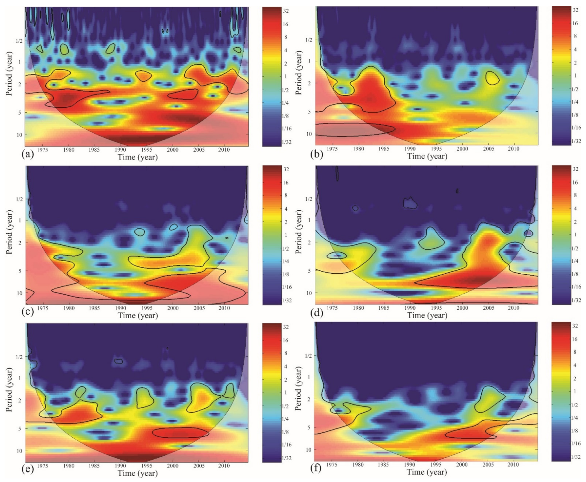
3.3. Wavelet Analysis

Multiresolution analysis provides information about frequency domains where the aquifer water levels might be related to precipitation or river levels, but provides no information about the temporal variability involved in the interaction process. Therefore, a wavelet technique was applied to identify the oscillation of the water level in aquifer and its possible responses to precipitation and river level variations in both the spatial and temporal domains. The interdecadal and interannual variability were investigated using 43 years of monthly data and 2 years of daily data.

(1)

Wavelet analysis of interdecadal variability

To eliminate the seasonal components from the hydrological time series, the 12-month moving average data during 1972 and 2014 were analysed using a wavelet analysis. The WPS of the monthly precipitation amount, average river level and aquifer water levels are shown in Figure 5a–f, respectively. The x- and y-axes represent the time-scale space. The z-axis represents the value of wavelet power, with low–high values shown in blue–red colours.

In the WPS for precipitation (Figure 5a), a high WPS was detected at periodicities of 2–7 and 11 years, indicating strong interdecadal variations in these frequency domains. High-power spectra were also observed in the 2–7- and 11-year bands for river levels (Figure 5b), but they were only concentrated in the period of 1972–1987. The WPS for water levels in the aquifer (Figure 5c–f) showed a similar distribution of wavelet power. Significant power spectra were observed in the 2–7 years band during 1972–1985 and 1995–2012. Significant power spectra with a periodicity of 11 years were only found for aquifer water levels in well w1.

The high CCF between precipitation and groundwater level at multiresolution level 9–10 was calculated in comparison with the river level, suggesting that precipitation was the main cause of interdecadal variability in aquifer water levels. The spatial and temporal features of coherence between precipitation and aquifer water levels were investigated using a WTC. Figure 6a–d shows the WTC between the monthly precipitation amount and water levels in the aquifer. The z-axis represents the value of the coherence, with low–high values in blue–red colours. The WTC highlighted a significant coherence between precipitation and aquifer water levels in the 2–5 years band during 1972–1988 and 1995–2012, and the 7 years band during 1990–2014. A significant coherence between precipitation and aquifer water levels, with a periodicity of 11 years, was only observed in well w3. The in-phase relationship dominated in the domains with significant coherence. Figure 6e–h shows the WTC between river level and aquifer water level in wells 1–4, respectively. A significant coherence was obtained in the 1–2 years band, and in-phase relationships were detected in these domains.

(2)

Wavelet analysis of interannual variability

To determine the interannual variability of aquifer water levels, the daily data during 2013 and 2014 were subjected to a wavelet analysis. The WPS of the daily precipitation amount, and average river and aquifer water levels, are shown in Figure 7a–f, respectively. The WPS for the daily precipitation amount (Figure 7a) indicated that a high-power spectrum mainly occurred during July and November in a hydrological year. The WPS for river and water levels in the aquifer (Figure 7b–f) had similar spectral distribution features to those of precipitation, indicating that a strong fluctuation occurred in these domains.

The WTC between the daily precipitation amount and aquifer water levels in the study area are presented in Figure 8a–d. In the low-frequency domains (less than 32 days), a discontinuous coherence was observed. There was a high coherence between precipitation and water levels in the aquifer that was concentrated in both the rainy and dry seasons, with periodicities of 64 and 128 days, respectively. For the periodicity of around 32 days, a significant coherence was obtained only in the rainy season (during July to December). Both in- and anti-phase relationships were observed in the domains with significant coherence. Figure 8e–h shows the WTC between river level and aquifer water level in wells 1–4, respectively. A significant coherence was obtained in almost all domains, and in-phase relationships were detected in these domains.

4. Discussion

4.1. Influences of Precipitation and River on Groundwater

The influence of precipitation and river level on groundwater was clearly demonstrated by the high CCF between precipitation/river level and groundwater level at different multiresolution levels. Both CCFs had their most significant peaks for an annual frequency, suggesting that seasonal variability dominates in the hydrological processes. The WPS for the 42-year monthly precipitation, river level and aquifer water level data (seasonal components removed) clearly displayed components with a periodicity of 2–7 years, suggesting that the interdecadal interactions might influence this periodicity. The WPS for the 2-year daily data showed significant or high-power spectra in the 4–128-days band during the rainy season, indicating that a strong hydraulic interaction might occur in the rainy season.

The spatial and temporal features of the interaction between precipitation and groundwater at the interdecadal time scale was analysed based on the monthly precipitation–groundwater WTC (Figure 6). Although a significant coherence was detected at a low frequency (less than 2 years), a low cross-interaction power was observed in these domains. Consequently, the interannual coherence displayed in Figure 6 is meaningless. The domains with a significant coherence between precipitation and groundwater (Figure 6) had a high consistency with domains with a significant or high-power spectra. This behaviour suggests that the interdecadal oscillation of shallow aquifer water levels is determined by planetary-scale atmospheric moisture circulation [3,6,14], and the precipitation in the study area reflects these moisture circulation processes. High CCFs between river level and groundwater (Table 3) were observed in levels 2–7, suggesting that the interdecadal variation in precipitation affects the groundwater and river levels in similar domains.

The influences of precipitation and river on groundwater at the interannual time scale were studied based on the daily precipitation/river level–groundwater WTC (Figure 8). A significant WTC was detected in the different spatial–temporal domains between precipitation and groundwater. However, the WPS for the daily precipitation and groundwater data suggested that a strong fluctuation in hydrological processes occurred in the rainy season, and in-phase relationships dominated in this period. This behaviour indicates that the effects of precipitation on the groundwater table mainly occur in the rainy season, and the phase differences can provide a reasonable estimate of the recharge-water travel time. The WTC between river level and groundwater revealed a significant coherence in almost all of the spatial–temporal domains. It could be inferred that the direct hydraulic connection between the river and aquifer occurred across diurnal to annual scales through both recharge and discharge processes. The recharge and discharge processes might be recognized by the direction of the arrows in the river level–groundwater WTC.

4.2. Recharge Travel Time

Precipitation recharge to the aquifer occurs with lags that can range from hours to days, and even months [12]. The recharge-water travel time in the study area was estimated from the pattern of the arrows in the precipitation–groundwater WTC at the interannual time scale (Figure 8). The results were consistent for each observation well in the study area. The results of the correlation between precipitation and groundwater in the different spatial and temporal domains indicated that the daily precipitation affected the groundwater at periodicities of 4–16 and 32–64 days during July and September in the study area. In 2013, the area of significant coherence with periodicities of 4–16 days had an in-phasing of about 1/8 of a cycle, suggesting a 1-day delay in the response of the aquifer to precipitation. The phase difference in the periodicities of 32–64 days equated to zero, and this pattern indicated no time lag existed at these time scales. In 2014, the arrow angles with significant coherence in the periodicities of 4–16 days ranged from −1/3 to −2/3 π, which indicated that the response time of the aquifer to precipitation was about 3–6 days. An in-phasing of about 5/6 of a cycle was detected in the periodicities of 32–64 days, indicating a time lag of about 40 days.

The precipitation led aquifer water levels by up to 6 days in the study area, which differed from other examples of semiconfined aquifers published in the literature [3,6]. This might be a result of the unconfined condition of the study aquifer. The different time lags of groundwater level to precipitation, with periodicities of 4–16 days during 2013 and 2014, might be due to the timing of maximum precipitation. The piezometric levels in the unconfined aquifer responded quickly to the variation in precipitation when the soil pores were not filled. The maximum precipitation occurred in late August in 2013 and early August in 2014, and this behaviour might cause a longer average travel time of precipitation to the aquifer in 2014. The time lags with periodicities of 32–64 days might be associated with other local climatic indices, such as barometric pressure, humidity and air temperature [3].

5. Conclusions

The influences of precipitation and river level on groundwater level in different spatial and temporal domains in the Yoshino River Basin, Japan, were assessed using a wavelet analysis. The interannual and interdecadal variability of the hydrological processes were identified using the WPS approach, and the interactions between precipitation, river and groundwater were analysed by multiresolution and WTC analyses. Compared with the spectral analysis, the wavelet technique provided an effective way to detect the correlations among precipitation, river level and aquifer level in the temporal domain. The detailed information of correlations among precipitation, groundwater level and river level provide an efficient implement to improve regional water-resource management efficiency.

The significant fluctuations in precipitation, river level and piezometric levels in the study area were mainly concentrated at periodicities of 4–128 days, 1 year and 2–7 years. The effects of precipitation and river level on piezometric levels were also observed in these periods. The correlation in the 1-year band was recognized as the seasonal variability of the hydrological processes. The significant interaction in the 4–128-days band mainly occurred in the rainy season, and the 2–7-year oscillation of aquifer water levels was determined by the variation in precipitation.

The recharge-water travel time in the study area was estimated from the pattern of arrows in the precipitation–groundwater WTC, and the results were consistent for each observation well. The precipitation led aquifer water levels by up to 6 days in the study area, and the response times of the aquifer to precipitation were 1 day and 3–6 days in 2013 and 2014, respectively. The different time lags of groundwater to precipitation might be caused by the timing of maximum precipitation. The piezometric levels in the unconfined aquifer responded quickly to the variation in precipitation when the soil pores were not filled. The maximum precipitation occurred in late August in 2013 and early August in 2014, which might have resulted in a longer precipitation travel time in 2014.

References

1. Taylor, R.G.; Scanlon, B.; Döll, P.; Rodell, M.; van Beek, R.; Wada, Y.; Longuevergne, L.; Leblanc, M.; Famiglietti, J.S.; Edmunds, M.; et al. Ground water and climate change. Nature Clm. Change 2013, 3, 322–329. [Google Scholar] [CrossRef] [Green Version]
2. Gribovszki, Z.; Szilágyi, J.; Kalicz, P. Diurnal fluctuations in shallow piezometric levels and streamflow rates and their interpretation—A review. J. Hydrol. 2010, 385, 371–383. [Google Scholar] [CrossRef] [Green Version]
3. Dong, L.; Shimada, J.; Kagabu, M.; Fu, C. Teleconnection and climatic oscillation in aquifer water level in Kumamoto plain, Japan. Hydrol. Process. 2015, 29, 1687–1703. [Google Scholar] [CrossRef]
4. Green, T.R.; Taniguchi, M.; Kooi, H.; Gurdak, J.J.; Allen, D.M.; Hiscock, K.M.; Treidel, H.; Aureli, A. Beneath the surface of global change: Impacts of climate change on groundwater. J. Hydrol. 2011, 405, 532–560. [Google Scholar] [CrossRef] [Green Version]
5. Fleming, S.W.; Quilty, E.J. Aquifer Responses to El Niño–Southern Oscillation, Southwest British Columbia. Groundwater 2006, 44, 595–599. [Google Scholar] [CrossRef]
6. Tremblay, L.; Larocque, M.; Anctil, F.; Rivard, C. Teleconnections and interannual variability in Canadian piezometric levels. J. Hydrol. 2011, 410, 178–188. [Google Scholar] [CrossRef]
7. Jiao, J.J.; Tang, Z. An analytical solution of groundwater response to tidal fluctuation in a leaky confined aquifer. Water Resour. Res. 1999, 35, 747–751. [Google Scholar] [CrossRef] [Green Version]
8. Dong, L.; Cheng, D.; Liu, J.; Zhang, P.; Ding, W. Analytical Analysis of Groundwater Responses to Estuarine and Oceanic Water Stage Variations Using Superposition Principle. J. Hydrol. Eng. 2016, 21, 04015046. [Google Scholar] [CrossRef]
9. Ghanbari, R.N.; Bravo, H.R. Coherence among Climate Signals, Precipitation, and Groundwater. Groundwater 2011, 49, 476–490. [Google Scholar] [CrossRef]
10. Shih, D.C.F.; Lee, C.D.; Chiou, K.F.; Tsai, S.M. Spectral analysis of tidal fluctuations in ground water level. J. Am. Water Resour. Assoc. 2000, 36, 1087–1099. [Google Scholar] [CrossRef]
11. Dong, L.; Shimada, J.; Kagabu, M.; Yang, H. Barometric and tidal-induced aquifer water level fluctuation near the Ariake Sea. Environ. Monit. Assess. 2015, 187, 1–16. [Google Scholar] [CrossRef] [PubMed]
12. Namdar Ghanbari, R.; Bravo, H.R. Evaluation of correlations between precipitation, groundwater fluctuations, and lake level fluctuations using spectral methods (Wisconsin, USA). Hydrogeol. J. 2011, 19, 801–810. [Google Scholar] [CrossRef]
13. Labat, D. Recent advances in wavelet analyses: Part 1. A review of concepts. J. Hydrol. 2005, 314, 275–288. [Google Scholar] [CrossRef]
14. Charlier, J.B.; Ladouche, B.; Maréchal, J.C. Identifying the impact of climate and anthropic pressures on karst aquifers using wavelet analysis. J. Hydrol. 2015, 523, 610–623. [Google Scholar] [CrossRef] [Green Version]
15. Mallat, S.G. A Theory for Multiresolution Signal Decomposition: The Wavelet Representation. IEEE Trans. Pattern Anal. Mach. Intell. 1989, 11, 674–693. [Google Scholar] [CrossRef] [Green Version]
16. Kumar, P.; Foufoula-Georgiou, E. Wavelet analysis for geophysical applications. Rev. Geophys. 1997, 35, 385–412. [Google Scholar] [CrossRef] [Green Version]
17. Lafrenière, M.; Sharp, M. Wavelet analysis of inter-annual variability in the runoff regimes of glacial and nival stream catchments, Bow Lake, Alberta. Hydrol. Process. 2003, 17, 1093–1118. [Google Scholar] [CrossRef]
18. Benke, K.K.; Lowell, K.E.; Hamilton, A.J. Parameter uncertainty, sensitivity analysis and prediction error in a water-balance hydrological model. Math. Comput. Model. 2008, 47, 1134–1149. [Google Scholar] [CrossRef]
19. Kang, S.; Lin, H. Wavelet analysis of hydrological and water quality signals in an agricultural watershed. J. Hydrol. 2007, 338, 1–14. [Google Scholar] [CrossRef]
20. Fu, C.; James, A.L.; Wachowiak, M.P. Analyzing the combined influence of solar activity and El Niño on streamflow across southern Canada. Water Resour. Res. 2012, 48. [Google Scholar] [CrossRef]
21. Massei, N.; Laignel, B.; Deloffre, J.; Mesquita, J.; Motelay, A.; Lafite, R.; Durand, A. Long-term hydrological changes of the Seine River flow (France) and their relation to the North Atlantic Oscillation over the period 1950–2008. Int. J. Climatol. 2010, 30, 2146–2154. [Google Scholar] [CrossRef]
22. Zhang, Q.; Xu, C.Y.; Jiang, T.; Wu, Y. Possible influence of ENSO on annual maximum streamflow of the Yangtze River, China. J. Hydrol. 2007, 333, 265–274. [Google Scholar] [CrossRef]
23. Torrence, C.; Compo, G.P. A Practical Guide to Wavelet Analysis. Bull. Am. Meteorol. Soc. 1998, 79, 61–78. [Google Scholar] [CrossRef] [Green Version]
24. Grinsted, A.; Moore, J.C.; Jevrejeva, S. Application of the cross wavelet transform and wavelet coherence to geophysical time series. Nonlinear Process. Geophys. 2004, 11, 561–566. [Google Scholar] [CrossRef]
25. Adamowski, J.F. River flow forecasting using wavelet and cross-wavelet transform models. Hydrol. Process. 2008, 22, 4877–4891. [Google Scholar] [CrossRef]
26. Liu, Y.; Brown, J.; Demargne, J.; Seo, D.J. A wavelet-based approach to assessing timing errors in hydrologic predictions. J. Hydrol. 2011, 397, 210–224. [Google Scholar] [CrossRef]
Figure 1. Location of the study area.
Water 14 00625 g001
Figure 2. The (a) precipitation, and piezometric levels (based on average sea level in Tokyo Bay) in observation wells (b) 1, (c) 2, (d) 3 and (e) 4, and (f) river levels from 1 January 1972 to 30 December 2014 in the study area.
Water 14 00625 g002
Figure 3. Annual precipitation amount, average groundwater level and river level from 1972 to 2014 in the study area.
Water 14 00625 g003
Figure 4. Multiresolution analysis results for (a) precipitation, (b) river level and (c) aquifer water level (taking well 1 as an example). The different components of the decomposition correspond (from top to bottom) with short- to long-time-scale processes, with level j corresponding to time scales at 2j1.
Water 14 00625 g004
Figure 5. Continuous wavelet spectra of monthly (a) precipitation, (b) river level and (c) piezometric levels in observation wells 1, (d) 2, (e) 3 and (f) 4 from 1972 to 2014 in the study area. The thick black contour designates the 5% significance level against red noise, whereas the lighter shade represents the cone of influence (COI), where edge effects might distort the picture.
Water 14 00625 g005
Figure 6. Wavelet coherences (WTCs) between the monthly precipitation and aquifer water level in (a) wells 1, (b) 2, (c) 3 and (d) 4, and WTCs between the monthly river water and aquifer water level in (e) wells 1, (f) 2, (g) 3 and (h) 4 from 1972 to 2014 in the study area. The thick black contour designates the 5% significance level against red noise, whereas the lighter shade represents the COI, where edge effects might distort the picture. The relative phase relationship is shown by the arrows (with the in-phase pointing right and the antiphase pointing left).
Water 14 00625 g006
Figure 7. Continuous wavelet spectra of daily (a) precipitation, (b) river level and (c) piezometric levels in observation wells 1, (d) 2, (e) 3 and (f) 4 during 2013 and 2014 in the study area. The thick black contour designates the 5% significance level against red noise, whereas the lighter shade represents the COI, where edge effects might distort the picture.
Water 14 00625 g007
Figure 8. The WTCs between the daily precipitation and groundwater level in (a) wells 1, (b) 2, (c) 3 and (d) 4, and WTCs between the daily river water and groundwater level in (e) wells 1, (f) 2, (g) 3 and (h) 4 from 2013 to 2014 in the study area. The thick black contour designates the 5% significance level against red noise, whereas the lighter shade represents the COI, where edge effects might distort the picture. The relative phase relationship is shown by the arrows (with the in-phase pointing right and the antiphase pointing left).
Water 14 00625 g008