Article

Simultaneous Estimation of a Contaminant Source and Hydraulic Conductivity Field by Combining an Iterative Ensemble Smoother and Sequential Gaussian Simulation

1
Department of Hydraulic Engineering, Tongji University, Shanghai 200092, China
2
State Key Laboratory of Hydrology-Water Resources and Hydraulic Engineering, Nanjing Hydraulic Research Institute, Nanjing 211100, China
3
Yangtze Ecology and Environment Corporation Limited, Wuhan 430015, China
4
School of Environment and Architecture, University of Shanghai for Science and Technology, Shanghai 200093, China
5
Key Laboratory of Agricultural Soil and Water Engineering in Arid and Semiarid Areas, Ministry of Education, Northwest A&F University, Yangling 712100, China
6
Shanghai Institute of Disaster Prevention and Relief, Tongji University, Shanghai 200092, China
*
Author to whom correspondence should be addressed.
Water 2022, 14(5), 757; https://doi.org/10.3390/w14050757
Submission received: 27 January 2022 / Revised: 21 February 2022 / Accepted: 25 February 2022 / Published: 27 February 2022
(This article belongs to the Section Hydrogeology)

Abstract

:
Joint estimation of groundwater contaminant source characteristics and hydraulic conductivity is of great significance for contaminant transport models in heterogeneous subsurface media. As for accurate characterization of hydraulic conductivities, both geostatistical modeling and groundwater inverse modeling are alternative approaches. In this study, an iterative ensemble smoother and sequential gaussian simulation (SGSIM) in geostatistics modeling were combined to realize the simultaneous inversion of contaminant sources and hydraulic conductivities, by using directly measured hydraulic conductivities and indirect hydraulic head and concentration data. To alleviate the high computational cost caused by repetitive evaluations of complex, high-dimensional groundwater models, SGSIM with the pilot points method was used. Considering the characteristics of the proposed method, four scenarios with ten cases were set up in terms of ensemble number and iteration number that affect the performance of the iterative ensemble smoother, the number of pilot points, and the observation data, respectively. The results for the synthetic example indicate that the ensemble size of 2000 and the pilot point number of 80 is an ideal combination of parameters, and the proposed method can successfully recover contaminant source information simultaneously with hydraulic conductivity.

1. Introduction

To implement the remediation strategy in the contaminated groundwater, it is critical to accurately estimate the key parameters (the location and strength of the contaminant sources) of the groundwater contaminant transport model. The hydraulic conductivity usually also needs to be identified because of its close relationship with the contaminant transport.
As for accurate characterization of hydraulic conductivities, geostatistical modeling is an effective solution to characterize spatial variability and predict the property of interest at unsampled locations. However, geostatistical methods based on directly measured hydraulic conductivities do not give good results at model validation [1]. For that reason, indirect observation data (hydraulic head and concentration data were further conditioned through a groundwater inverse model [2,3]. Data assimilation, also known as a stochastic inverse method, in which the parameters of groundwater model are considered as random variables, rather than updating the specific values of the model parameters in the optimization method, have been widely used in hydrogeology. The probability distribution used to characterize these random variables is updated with the observation data [4,5,6,7].
An ensemble Kalman Filter (EnKF) proposed by Evensen (2003) [8], as an ensemble-based data assimilation method, can update model parameters and state variables by sequentially assimilating available measurements and has gained popularity in multidisciplinary fields such as meteorology and hydrology [9,10]. An alternative data assimilation method to the EnKF is the Ensemble Smoother (ES) [11], and this has emerged as an effective and efficient approach for data assimilation [4,12,13].
To improve the applicability and efficiency of an ensemble smoother for strongly nonlinear problems, Zhang et al. (2018) proposed an iterative local updating ensemble smoother (ILUES) [6], in which the local ensemble of each sample is defined by measuring the distance from this sample and making observations, and each sample is updated locally using the scheme of ES instead of updating globally. Additionally, to avoid the strong non-linearity impact on the data match quality, the same set of observation data is assimilated multiple times to update the parameters by introducing the iterative scheme of the ensemble smoother. In this study, the ILUES algorithm is adopted as the inversion framework to estimate the contaminant source characteristics and hydraulic conductivities, among which a geostatistical modeling method named sequential gaussian simulation (SGSIM) is employed for gaussian random field generation.
In this paper, the identification of contaminant sources and estimation of hydraulic conductivities are simultaneously carried out. As complex groundwater inverse models have high-dimensional characteristics, the hydraulic conductivities cannot be retrieved efficiently. To alleviate the high computational cost caused by repetitive evaluations of complex, high-dimensional groundwater models, estimation of hydraulic conductivity at selected pilot points was a feasible approach [14]. The objective of this study is to combine a data assimilation algorithm and geostatistical approach to realize the simultaneous inversion of contaminant sources and hydraulic conductivity field by leveraging directly measured hydraulic conductivities and indirect hydraulic head and concentration data.
The remainder of this paper is organized as follows. Section 2 presents the detailed description of groundwater flow and the contaminant transport model. Section 3 outlines the framework of the proposed inversion methodology. In Section 4, results obtained from numerical experiments are discussed. Some conclusions are given in Section 5.

2. Problem Formulation

The transport of contaminants in saturated aquifers may involve diffusion, advection, dispersion, absorption. In this study, advection and dispersion are dominated processes in a two-dimensional contaminant transport system under steady-state groundwater flow conditions.
The governing equation for the steady-state groundwater flow can be written as follows:
x K h x = 0
and the flow velocity v (LT−1) can be obtained by Darcy’s law:
v = K θ h x
where h (L) is the hydraulic head; K (LT−1) represents the hydraulic conductivity; θ is effective porosity (dimensionless); The flow governing equation is solved by numerical simulator MODFLOW [15]. Then, the resulting velocity v is used as input for the advection–dispersion equation to calculate the contaminant concentration by MT3DMS [16]. The advection–dispersion equation for a 2D saturated aquifer is:
b C t = x b D C x x b v C + C s W θ
where t (T) is time; b (L) is the saturated thickness of aquifer; C (ML−3) is the concentration of the dissolved chemical species; Cs (ML−3) is the concentration of source or sink; W (LT−1) is the volumetric flux per unit area; D (L2T−1) is the hydrodynamic dispersion coefficient, determined by v, and longitudinal and transverse dispersivities ( α L and α T ) (L).

3. Methodology

The ability to obtain accurate key parameters (the location and strength of contaminant source, hydraulic conductivities of aquifers, etc.) of groundwater contaminant transport models determines the accuracy of contaminant transport predictions, which further affects groundwater management and environmental assessment of groundwater pollution. The goal of this study is to estimate the contaminant parameters (the location and strength of contaminant sources) and hydraulic conductivities simultaneously, by using directly measured hydraulic conductivities and indirect hydraulic head and concentration data.
An inverse problem with high-dimensional inputs may result in heavy computational burden due to repeatedly running forward models to obtain satisfactory results. Thus, to improve the computational efficiency of groundwater inverse problems, the pilot points methods incorporating prior information [17] was adopted.
In this paper, a modified iterative ensemble smoother (ILUES) was adopted as the inversion framework for solving groundwater inverse problems, and a geostatistical method named sequential gaussian simulation (SGSIM) was employed for generating realizations of Gaussian random fields. To summarize, our proposed method (SGSIM-ILUES) is based on the coupling of ILUES and SGSIM. A brief description of the steps of the proposed method are below.
For simplicity, the relationship between model parameters and measurements can be expressed in the following form:
d = f m + ε
where d is a Nd × 1 vector for measurements, m is the vector for model parameters, f(m) is the prediction from the forward model, and ε is the vector for Gaussian-distributed measurement errors.
For convivence, matrix M and D are introduced. M f = m 1 f , m 2 f , , m N e f is an ensemble of Ne parameter samples randomly drawn from the prior distribution, and M a = m 1 a , m 2 a , , m N e a is the updated ensemble conditioned on the measurement d. D f = f m 1 f , f m 2 f , , f m N e f and D a = f m 1 a , f m 2 a , , f m N e a are output ensemble corresponding to M f and M a by evaluating the forward model.
 Step 1 
Set iteration counter i = 1.
 Step 2 
Generate input ensemble M f from the prior distribution.
In the input ensemble M = ln K C s , K is the ensemble of log-hydraulic conductivities at pilot points, and Cs is the contaminant source parameters.
(a)
Based on n h d directly measured hydraulic conductivities (hard data) generated Ne realizations of hydraulic conductivity field; the hydraulic conductivity value at n p pilot points was obtained from Ne realizations of the hydraulic conductivity field.
(b)
An initial ensemble of contaminant source parameters was generated by sampling from priori distribution of contaminant source parameters (the location and strength of contaminant source for each stress period).
 Step 3 
Generate output ensemble D f by evaluating the forward model.
Based on the hydraulic conductivities at pilot points and hard data, the SGSIM method is used to interpolate to unsampled locations, to thus obtain Ne realizations of the hydraulic conductivity field. A detailed explanation of the SGSIM can be found in [18].
An ensemble of contaminant source parameters, together with Ne realizations of the hydraulic conductivity field, are jointly used as inputs to the forward model (MODFLOW and MT3DMS simulators) to obtain D f (simulated heads and concentrations).
 Step 4 
Obtain the update ensemble M a = ln K C s using ILUES algorithm.
A detailed explanation of Iterative Local Updating Ensemble Smoother (ILUES) can be found in [6].
 Step 5 
Set i = i + 1. If i = N i t e r , stop; otherwise, let M f = M a , go to Step 3.

4. Illustrative Example

4.1. Problem Description

In this study, advection and dispersion are dominated processes in a two-dimensional contaminant transport system under steady-state groundwater flow conditions. The hypothetical aquifer is a saturated and confined aquifer with a 2D steady-state groundwater flow (Figure 1). Specifically, the aquifer size is 40 m in the x-direction and 20 m in the y-direction. The top and bottom boundary is no-flux. The constant hydraulic heads of 12.00 m and 10.00 m are the west and east boundary, respectively, and the aquifer thickness was 1 m. The values for aquifer parameters are listed in Table 1.
Considering the spatial heterogeneity, the reference conductivity field (in Figure 1) is lognormally distributed with mean = 3.0 and variation = 1.0, and the correlation length along x and y directions are 8.0 m and 4.0 m, respectively. The reference hydraulic conductivity field was generated based on known hydraulic conductivity of hard data using SGSIM method.
In this hypothetical aquifer, some amount of contaminant was released from a point source. The contaminant source is characterized by ten parameters, i.e., Sx, Sy, S P i (MT−1) (mass-loading rate) during the i th stress periods, for i = 1, …, 8 as listed in Table 2. The whole simulation time is 40 days that is equally divided into eight stress periods, that is, 5 days for each period. The simulation mode for MODFLOW and MT3DMS is steady-state and transient, respectively. Consequently, 10 unknown contaminant source parameters and hydraulic conductivities at n p pilot points need to be estimated.

4.2. Assessment Criteria

To quantitatively evaluate the estimation results, the root mean square error (RMSE) and average ensemble spread (AES) are introduced as assessment criteria. The RMSE measures the match between the reference and estimated parameters and is defined as:
RMSE = i = 1 N x V ^ e s t i V a c t i 2 N x
The AES measures the uncertainty or confidence of the estimated values of parameters, which can be expressed as:
AES = i = 1 N x 1 N e j = 1 N e V e s t i j V ^ e s t i 2 N x
where V ^ e s t i denotes the estimated value of parameter i, V a c t i represents the true value of parameter i, V e s t i j is the estimated value of parameter i in ensemble j, N x is the total number of estimated parameters. It should be noted that the lower the RMSE is, the more accurate the parameter estimation.

5. Results and Discussions

Considering the characteristics of the proposed methodology (in Section 3), Scenario 0, 1, 2, and 3 were set up in terms of ensemble number (Ne) and iteration number (Niter) that affect the performance of the ILUES algorithm, the number of pilot points ( n p ) of the SGSIM method, and the observation data, respectively.
In this section, there are ten discussion cases in total for all scenarios (Table 3). It is noted that in Case 1 only 20 measured conductivities (K), as hard data, were conditioned through the SGSIM method. In other cases, measured conductivities (K), hydraulic head and concentration data collected from observation wells, together with the conductivities at pilot points, were used to update the conductivities ensemble and contaminant source parameters.

5.1. Scenario 1

In this scenario, twenty measured conductivities were conditioned through the SGSIM method. Three posterior realizations (Figure 2b–d) of the log-transformed conductivity field showed some similarity to the reference field (Figure 2a). However, the calibrated high/low K zone deviated from the reference field. Moreover, resulting variance at the locations of measured conductivities was zero, and gradually elevated away from the conditioning points.

5.2. Scenario 2

In this scenario, besides the measured conductivities, hydraulic head and concentration data collected from observation wells were used to identify the conductivities. Hydraulic head measurements were taken once at observation wells as shown in Figure 1, while contaminant concentration measurements were collected every 4 days (ti = 4, 8, …, 40 day).
A number of assimilations utilizing the SGSIM-ILUES algorithm were performed, with the ensembles vary in size from 500 to 2000 (Case 2.1, 2.2, and 2.3). Specifically, the algorithm factors α and β were fixed to be 0.1 and 1 as suggested in [6]. For this scenario, the number of pilot points was fixed to be 80.
The identification results for source location and strength identification were obtained by using ensemble size from 500 to 3000, which demonstrates that source identification problem could be solved without using a fairly large size of ensemble in the SGSIM-ILUES algorithm. The RMSE values obtained for source location and strength identification were reduced by 85.86% when using 3000 ensembles instead of 500 (Figure 3a). Similarly, the utilization of 3000 ensemble members for log-transformed conductivity estimation at pilot points led to about 76.61% reduction in the RMSE values compared with that adopting only 500 ensembles (Figure 3b). The AES value significantly decreased when the ensemble size increased from 500 to 2000, while it fluctuated slightly and followed a similar trend without obvious reduction as the ensemble size increased from 2000 to 3000 for both source identification (Figure 3a) and log-transformed conductivity estimation at pilot points (Figure 3b).
Meanwhile, as the number of ensemble members reached 3000, the AES value was gradually becoming stable at 0.1512 and 0.0932 after SGSIM-ILUES assimilation for source identification and log-conductivity estimation, respectively. Note that the required CPU time and storage necessary for running the SGSIM-ILUES assimilation scheme using 3000 ensembles could be much higher compared to using only 500 ensembles. To strike a balance between the computational efficiency and accuracy, an ensemble size of 2000 might be a reasonable choice for this study.
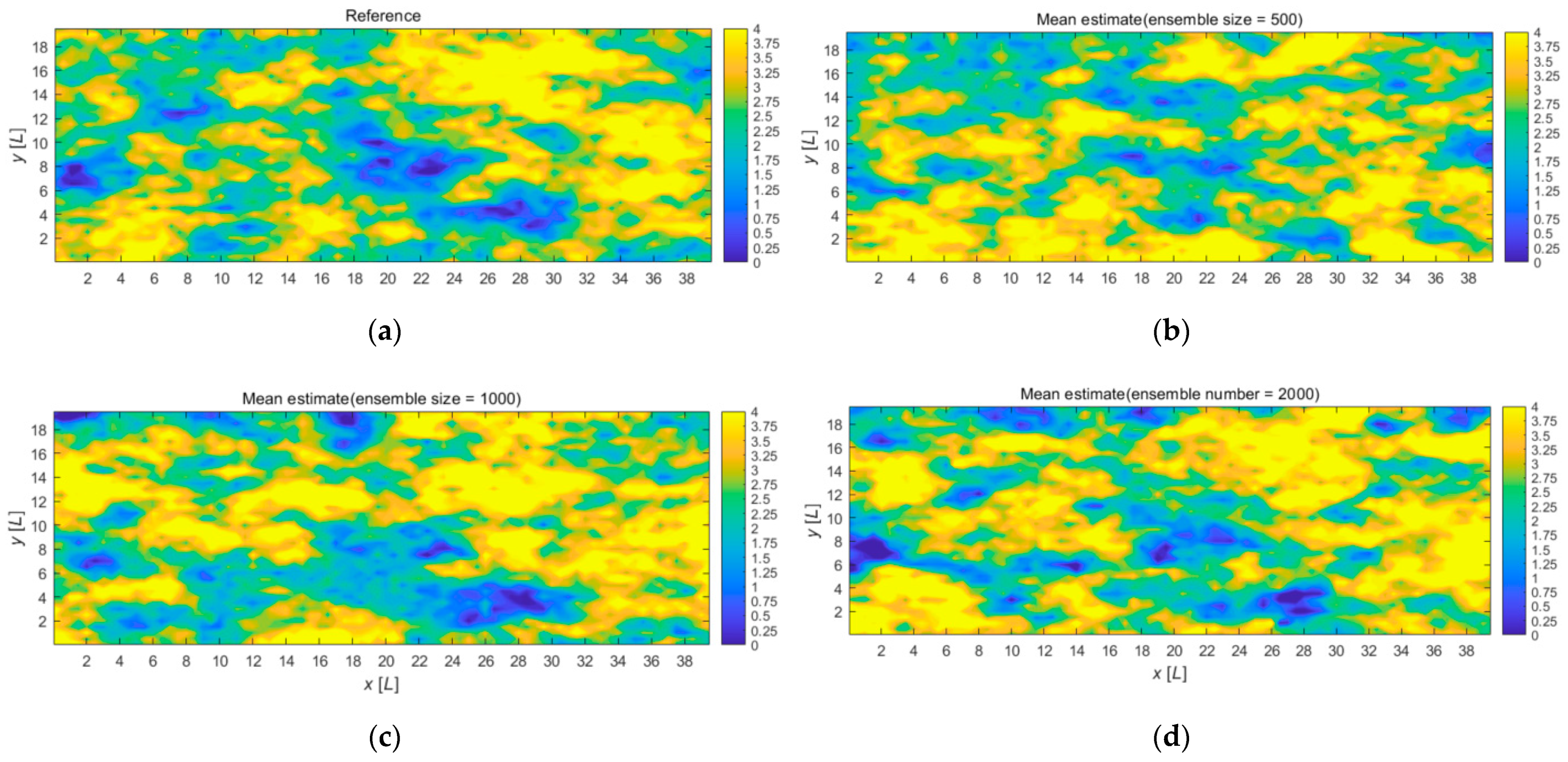
As shown in Figure 4, compared with the reference log-transformed conductivity field, with the increase in ensemble size from 500 to 2000, the accuracy of the estimated log-conductivity field was improved. This is expected because the distribution of the log-conductivity field is better depicted by the iterative ensemble smoother with larger ensembles.
In addition to ensemble number (Ne), iteration number (Niter) also affected the solution of groundwater inverse problems. Here, Case 2.3 was chosen to study the effect of iteration number, and the trace plots of the 10 contaminant source characteristics (in Table 2) versus the iteration number are shown in Figure 5. It could be concluded that after six iterations the identification of contaminant source characteristics in terms of source locations and source strengths were achieved. To ensure convergence, a slightly larger number of Niter = 8 was chosen in the subsequent study.

5.3. Scenario 3

In this scenario, direct data (20 measured conductivities) and indirect data (hydraulic head and concentration data) were exactly the same as in Scenario 2. A number of assimilations utilizing the SGSIM-ILUES algorithm were performed and pilot points vary from 40 to 120 (Case 2.3, 3.1, and 3.2). Specifically, the algorithm factors α and β were also fixed to be 0.1 and 1. According to the results of Scenario 2, the ensemble number (Ne) was fixed to be 2000 in this scenario.
As shown in Figure 6, compared with the reference log-transformed conductivity field, the ensemble mean was improved from Case 3.1 to Case 2.3, because the elevated number of pilot points from 40 to 80 brought more information. As the pilot point number increased from 80 to 120, the accuracy of estimated log-conductivity field was not improved significantly. This meant that additional information from more pilot points could not further improve the accuracy of the estimates.
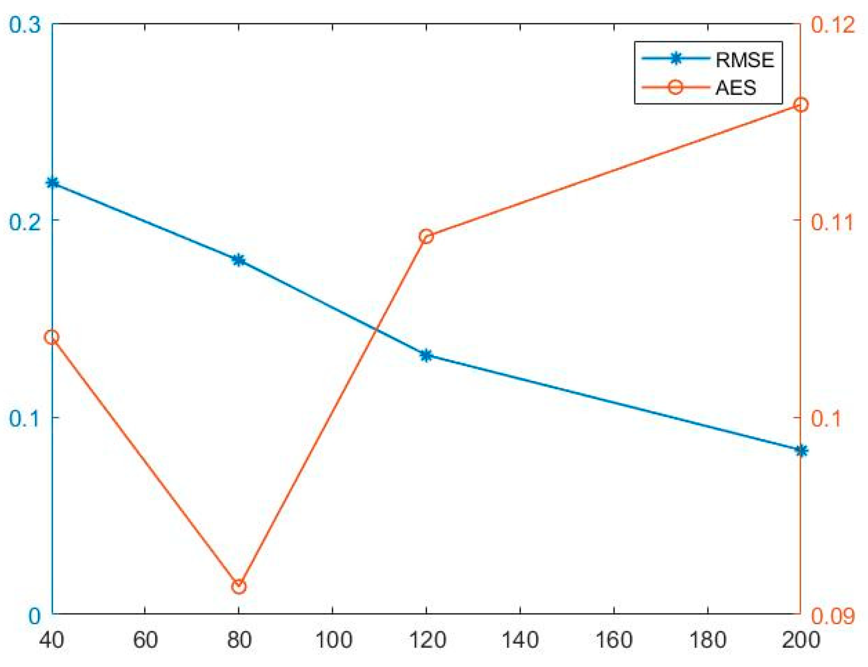
The RMSE value obtained for log-transformed conductivities estimation at pilot points was reduced by 61.90% when using 200 pilot points instead of 40 (Figure 7). As shown in Figure 7, the AES value significantly decreased when the pilot point number increased from 40 to 80, and it increased significantly as the pilot point number increased from 80 to 200. This meant that the elevated number of pilot points might introduce noises while bringing more additional information. To strike a balance between the information and noises from pilot points, the number of pilot points (np = 80) might be a reasonable choice for this study.

5.4. Scenario 4

In this scenario, three temporal distributions of indirect data (hydraulic head and concentration data) were compared. The first case was Case 2.3 with contaminant concentration measurements collected every 4 days (ti = 4, 8, …, 40 day), the second case was Case 4.1 with contaminant concentration measurements collected only in the last 10 days (ti = 31, 32, …, 40 day), and the third case was Case 4.2 with contaminant concentration measurements collected every 8 days (ti = 8, 16, …, 40 day).
Specifically, the algorithm factors α and β were also fixed as 0.1 and 1. According to the results of Scenario 2 and 3, the ensemble number (Ne) and the number of pilot points (np) were fixed as 2000 and 80 in this scenario.
After the assimilation procedure of SGSIM-ILUES algorithm, the trace plots of the identification results for contaminant source characteristics (for simplify, only Sy, SP3 and SP8 were selected) versus the iteration number with three different patterns of observations were plotted in Figure 8. Moreover, the resulting mean estimate and variance of log-hydraulic conductivity fields with different observations settings were shown in Figure 9.
We first investigated the influence of temporal distribution of observation on the SGSIM-ILUES performance in this scenario, where the total number of measurements was fixed. The SGSIM-ILUES scheme assimilating the hydraulic head and contaminant concentration data collected every 4 days (Figure 8a) clearly outperformed that assimilating the data collected in the last 10 days (Figure 8b) in terms of the identification results of source characteristics involving source locations (Sy) and source strengths (SP3 and SP8). Meanwhile, compared to Case 4.1 (Figure 9d,e), the estimated hydraulic conductivities in Case 2.3 (Figure 9b,c) had a more accurate mean estimate and lower variance field. The main reason is as follows: compared with Case 4.1, which only used the observation information of the last 10 days, the observation information of Case 2.3 covered the complete stress periods, and could provide more data information for data assimilation under the condition of the same amount of observation information.
To explore the impact of the number of measurements on the joint estimation of source information and hydraulic parameters, the SGSIM-ILUES algorithm was employed to assimilate data collected every 4 days (ti = 4, 8, …, 40 day) and collected every 8 days (ti = 8, 16, …, 40 day), respectively. Figure 8a,c indicate that the contaminant source strength (SP3 and SP8) could be identified accurately both 220 and 120 observation data (Case 2.3 and Case 4.2). However, for y coordinate (Sy), the closer identification values to the true and less uncertainties were obtained by SGSIM-ILUES in Case 2.3. As shown in Figure 9, the assimilation results using 220 observation data (Figure 9b) could better represent the structures (high/low K zone) of the study domain. The lower variance field of estimated log-hydraulic conductivity could be obtained through assimilating data collected every 4 days (Figure 9c) in comparison with that obtained by assimilating data collected every 8 days (Figure 9g).
The above study results indicated that both the temporal distribution and number of observations influenced the performance of the joint estimation of source characteristics and hydraulic conductivity field by the proposed SGSIM-ILUES algorithm.

6. Conclusions

  • In this study, the iterative local updating ensemble smoother (ILUES) and sequential gaussian simulation (SGSIM) in geostatistics were combined to realize the simultaneous inversion of contaminant sources and hydraulic conductivity field. As an efficient data assimilation method, the ILUES algorithm was adopted to construct the framework for solving groundwater inverse problems. Specifically, the inversion of hydraulic conductivities was converted to the estimation of hydraulic conductivity at pilot points;
  • With the increasing ensemble size, our proposed method can obtain more accurate estimation of both source characteristics and the hydraulic conductivity field. Furthermore, too large an ensemble size may result in heavy computational burden, and the sensitivity of estimation results to the ensemble size becomes weak. For this study, the ensemble size of 2000 is sufficient to provide satisfactory results;
  • With the increasing number of pilot points, the RMSE metric decreases monotonically, but the AES metric characterizing the uncertainty or confidence of the estimation tends to first decrease and then increase. Perhaps it can be explained that the elevated number of pilot point introduce noises while bringing more additional information. For this study, the pilot point number of 80 might be a reasonable choice for this study;
  • The temporal distribution of measurements influences the identification of contaminant source parameter and hydraulic conductivities. To some extent, the proposed method performs better with the increase in the observations. Specially, the propose method performs better with the increase in the overlapping degree of monitoring time and pollution occurrence. For this study, the inversion results by assimilating the hydraulic head and contaminant concentration data collected every 4 days clearly outperforms that by assimilating the data collected in the last 10 days.

Author Contributions

Conceptualization, S.J. and M.Z.; methodology, J.L. and X.X.; validation, R.Z. and X.L.; formal analysis, S.J. and X.X.; data curation, R.Z. and J.L.; writing—original draft preparation, S.J.; writing—review and editing, X.X. and M.Z.; visualization, X.X.; funding acquisition, M.Z. and S.J. All authors have read and agreed to the published version of the manuscript.

Funding

This work was supported by the Belt and Road Special Foundation of the State Key Laboratory of Hydrology-Water Resources and Hydraulic Engineering (No. 2019nkzd01), the Shanghai Science and Technology Innovation Action Plan Program, China (No. 21DZ1201205), and National Natural Science Foundation of China (42077176).

Data Availability Statement

Data and Matlab codes of this study are available upon request to the corresponding author.

Conflicts of Interest

The authors declare no conflict of interest. The funders had no role in the design of the study; in the collection, analyses, or interpretation of data; in the writing of the manuscript, or in the decision to publish the results.

References

  1. Lee, S.; Carle, S.F.; Fogg, G.E. Geologic heterogeneity and a comparison of two geostatistical models: Sequential Gaussian and transition probability-based geostatistical simulation. Adv. Water Resour. 2007, 30, 1914–1932. [Google Scholar] [CrossRef]
  2. Bailey, R.T.; Baù, D. Estimating geostatistical parameters and spatially-variable hydraulic conductivity within a catchment system using an ensemble smoother. Hydrol. Earth Syst. Sci. 2012, 16, 287–304. [Google Scholar] [CrossRef] [Green Version]
  3. Cao, Z.; Li, L.; Chen, K. Bridging iterative Ensemble Smoother and multiple-point geostatistics for better flow and transport modeling. J. Hydrol. 2018, 565, 411–421. [Google Scholar] [CrossRef]
  4. Bailey, R.; Baù, D. Ensemble smoother assimilation of hydraulic head and return flow data to estimate hydraulic conductivity distribution. Water Resour. Res. 2010, 46. [Google Scholar] [CrossRef]
  5. Erdal, D.; Cirpka, O.A. Joint inference of groundwater–recharge and hydraulic–conductivity fields from head data using the ensemble Kalman filter. Hydrol. Earth Syst. Sci. 2016, 20, 555–569. [Google Scholar] [CrossRef] [Green Version]
  6. Zhang, J.; Lin, G.; Li, W.; Wu, L.; Zeng, L. An Iterative Local Updating Ensemble Smoother for Estimation and Uncertainty Assessment of Hydrologic Model Parameters with Multimodal Distributions. Water Resour. Res. 2018, 54, 1716–1733. [Google Scholar] [CrossRef]
  7. Zhou, H.; Gómez-Hernández, J.; Li, L. Inverse methods in hydrogeology: Evolution and recent trends. Adv. Water Resour. 2014, 63, 22–37. [Google Scholar] [CrossRef] [Green Version]
  8. Evensen, G. The Ensemble Kalman Filter: Theoretical formulation and practical implementation. Ocean Dynam. 2003, 53, 343–367. [Google Scholar] [CrossRef]
  9. Franssen, H.J.H.; Kinzelbach, W. Ensemble Kalman filtering versus sequential self-calibration for inverse modelling of dynamic groundwater flow systems. J. Hydrol. 2009, 365, 261–274. [Google Scholar] [CrossRef]
  10. Houtekamer, P.L.; Zhang, F. Review of the Ensemble Kalman Filter for Atmospheric Data Assimilation. Mon. Weather Rev. 2016, 144, 4489–4532. [Google Scholar] [CrossRef]
  11. Leeuwen, P.; Evensen, G. Data assimilation and inverse methods in terms of a probabilistic formulation. Mon. Weather Rev. 1996, 124, 2898–2913. [Google Scholar] [CrossRef]
  12. Ju, L.; Zhang, J.; Meng, L.; Wu, L.; Zeng, L. An adaptive Gaussian process-based iterative ensemble smoother for data assimilation. Adv. Water Resour. 2018, 115, 125–135. [Google Scholar] [CrossRef]
  13. Li, L.; Stetler, L.; Cao, Z.; Davis, A. An iterative normal-score ensemble smoother for dealing with non-Gaussianity in data assimilation. J. Hydrol. 2018, 567, 759–766. [Google Scholar] [CrossRef]
  14. RamaRao, B.S.; LaVenue, A.M.; Marsily, G.D.; Marietta, M.G. Pilot Point Methodology for Automated Calibration of an Ensemble of conditionally Simulated Transmissivity Fields: 1. Theory and Computational Experiments. Water Resour. Res. 1995, 31, 475–493. [Google Scholar] [CrossRef]
  15. Harbaugh, A.W.; Banta, E.R.; Hill, M.C.; McDonald, M.G. MODFLOW-2000, The U.S. Geological Survey Modular Ground-Water Model—User Guide to Modularization Concepts and the Ground-Water Flow Process; Open-File Report; U.S. Geological Survey: Reston, VI, USA, 2000. [Google Scholar]
  16. Zheng, C.; Wang, P.P. MT3DMS: A Modular Three-Dimensional Multispecies Transport Model for Simulation of Advection, Dispersion, and Chemical Reactions of Contaminants in Groundwater Systems; Documentation and User’s Guide; Engineer Research and Development Center: Vicksburg, MS, USA, 1999. [Google Scholar]
  17. Alcolea, A.; Carrera, J.; Medina, A. Pilot points method incorporating prior information for solving the groundwater flow inverse problem. Adv. Water Resour. 2006, 29, 1678–1689. [Google Scholar] [CrossRef]
  18. Deutsch, C.V.; Journel, A.G. GSLIB:* Geostatistical Software Library and Users Guide; Oxford University Press: Oxford, UK, 1998. [Google Scholar]
Figure 1. The reference hydraulic conductivity with location of contaminant sources and observation wells. The red pentagram and the red dashed rectangle denote the contaminant source and potential area of the source, respectively. The black circles denote the observation locations.
Water 14 00757 g001
Figure 2. (a) The reference log-transformed conductivity field, (bd) three posterior realizations of the log-transformed conductivity field, (e) mean estimate of the log-transformed conductivity filed, and (f) estimation variance of the log-transformed conductivity field.
Water 14 00757 g002aWater 14 00757 g002b
Figure 3. RMSE (blue dots) and AES (orange dots) values resulting from the SGSIM-ILUES with different ensemble sizes, (a): for source location and source strength identification; (b): for log-transformed conductivity estimation at pilot points.
Water 14 00757 g003
Figure 4. The reference log-transformed conductivity field and estimated fields with different ensemble sizes in Scenario 1, (a): reference log-conductivity field; (b): ensemble size = 500; (c): ensemble size = 1000; (d): ensemble size = 2000.
Water 14 00757 g004
Figure 5. Trace plots of the source location and source strength at each iteration. (aj): Sx, Sy, and SPi during the ith stress periods, for i = 1, …, 8.
Water 14 00757 g005
Figure 6. The reference log-transformed conductivity field and estimated fields with different pilot point numbers in Scenario 3, (a): reference log-conductivity field; (b): pilot point number = 40; (c): pilot point number = 80; (d): pilot point number = 120.
Water 14 00757 g006
Figure 7. RMSE (blue dots) and AES (orange dots) values resulting from the SGSIM-ILUES with the pilot point number for log-transformed conductivity estimation at pilot points.
Water 14 00757 g007
Figure 8. Trace plots of the source location coordinates and source strength at the 3rd and 8th stress periods with different temporal distributions of hydraulic head and concentration data: (a) measurements are collected every 4 days, (b) measurements are collected only in the last 10 days, (c) measurements are collected every 8 days.
Water 14 00757 g008
Figure 9. The reference log-conductivity field (a) and estimated mean and variance fields with different temporal distributions of head and concentration data: (b,c) measurements collected every 4 days, (d,e) measurements collected only in the last 10 days, (f,g) measurements collected every 8 days.
Water 14 00757 g009
Table 1. Hydrogeological characteristics of the hypothetical aquifer.
ParameterUnitsValue
Grid sizem × m0.5 × 0.5
Aquifer thicknessm1.0
Effective porositynone0.30
Longitudinal dispersivitym2.0
Transverse dispersivitym0.6
Simulation timeday40
Table 2. Actual values of the source strength and prior range.
Contaminant ParameterPrior RangeActual Value
Sx (m)[1.25–10.25]2.25
Sy (m)[7.75–13.75]10.25
S P 1 (kg/d)[35–75]50
S P 2 (kg/d)[35–75]48
S P 3 (kg/d)[30–70]45
S P 4 (kg/d)[30–60]40
S P 5 (kg/d)[25–55]36
S P 6 (kg/d)[22–45]30
S P 7 (kg/d)[15–30]20
S P 8 (kg/d)[7–15]10
Table 3. Discussion cases for all scenarios.
Scenario No.Case No.Conditioned
K
Conditioned
h+C
Number of pp
(Np)
MethodEnsemble Size
Scenario 1Case 120SGSIM
Scenario 2Case 2.12022080SGSIM-ILUES500
Case 2.22022080SGSIM-ILUES1000
Case 2.32022080SGSIM-ILUES2000
Scenario 3Case 2.32022080SGSIM-ILUES2000
Case 3.12022040SGSIM-ILUES2000
Case 3.220220120SGSIM-ILUES2000
Scenario 4Case 2.32022080SGSIM-ILUES2000
Case 4.120220 *80SGSIM-ILUES2000
Case 4.22012080SGSIM-ILUES2000
* measurements are collected only in the last 10 days.
Publisher’s Note: MDPI stays neutral with regard to jurisdictional claims in published maps and institutional affiliations.