1. Introduction
Hazard maps of a debris flow can be obtained through two major kinds of methods: Empirical methods based on analysis of historical events and numerical methods using physically based equations [
1,
2]. An empirical method often uses correlations between the debris flow runout and topographic parameters, sediment supply, or dynamic parameters to make a prediction [
3,
4]. There are three major factors influencing the debris flow runout distance: The volume of removable sediment, catchment area, and internal relief [
5]. Zhou et al. [
6] established a multivariate relationship between runout distance and the debris volume or the internal catchment relief.
While empirical methods are useful to make hazard assessments at a regional scale, the positive prediction accuracy of the runout area covered by debris-flow deposits may be less than 40% [
7,
8]. Furthermore, empirical methods cannot provide comprehensive information on the processes of debris flows and the final deposit topography [
9]. An accurate prediction of the potentially exposed areas can be fundamental for the safety of human lives. The numerical methods can overcome some of these limitations, as they can reproduce the debris flow process through physical equations.
Two kinds of rheological closure models are commonly used in numerical simulation: Single-phase flow models and two-phase flow models. Single-phase flow models are commonly based on the Bingham rheology [
10], the Voellmy rheology [
11,
12], and the Bagnold rheology [
13,
14]. O’Brien et al. [
15] designed a two-dimensional (2D) mudflow program FLO-2D based on the Bingham rheology, and Beguería et al. [
16] designed a GIS-based debris flow program Massmove2D based on the Voellmy rheology. Ouyang et al. [
17] designed the two-dimensional debris flow program Massflow based on Coulomb and Voellmy frictional laws. Takahashi [
18] proposed a 2D granular flow model based on the Bagnold rheology and coupled with Coulomb flow resistance. Then, several modified granular models were developed by researchers [
19,
20,
21,
22,
23]. Based on Bagnold rheology, a new particle shear stress equation is derived for a wide range of particle flows [
24]. The equation was used to establish the continuum granular model Flow-3D [
25], which yielded promising results for the simulation of debris flow behavior [
26,
27].
Two-phase flow models mainly include the flow model composed of solid–fluid mixtures [
28,
29,
30], two-fluid debris flow model [
31,
32], general two-phase debris flow model [
33], Euler–Euler model [
34], a depth-averaged two-phase model [
35], and the depth-integrated model [
36]. The general two-phase debris flow model allows smooth transitions between non-viscous flow, hyper-concentrated sediment-laden flow, and debris flows. Moreover, Bout et al. [
37] developed OpenLISEM for the debris flow simulation. OpenLISEM couples the two-phase debris flow equations and a full hydrological catchment model. It can recreate the impact of both floods and debris flow runout. Furthermore, it involves simulating runoff, entrainment of sediment, and the formation of debris flow from intense erosion. In this paper, we call OpenLISEM without a full hydrological catchment model OpenLISEM_A, and we call OpenLISEM with a full hydrological catchment model OpenLISEM_B.
In this work, the single-phase flow models Massflow and Flow-3D and the two-phase flow models OpenLISEM_A and OpenLISEM_B were used to reproduce the process and depositional topography of debris flow. Two debris flow events occurred in the Wayao catchment in 2013 and 2020, and both debris flows were initiated from runoff. The topography of debris fan, erosion depth of channel deposition, and debris flow density were collected to calibrate simulation parameters and verify prediction ability. First, the four models were applied to reproduce the debris flow event in 2013. Second, the four models were used to predict the debris flow event in 2020, and the same set of parameters as the debris flow in 2013 is adopted, which is considered satisfactory. The prediction abilities of the four models are validated from the transport process and accumulation characteristics of the 2020 debris flow. The purposes are to discuss the advantages and limitations of the different models for debris flow prediction and provide suggestions for the physically based hazard assessments in mountainous areas.
2. Study Sample
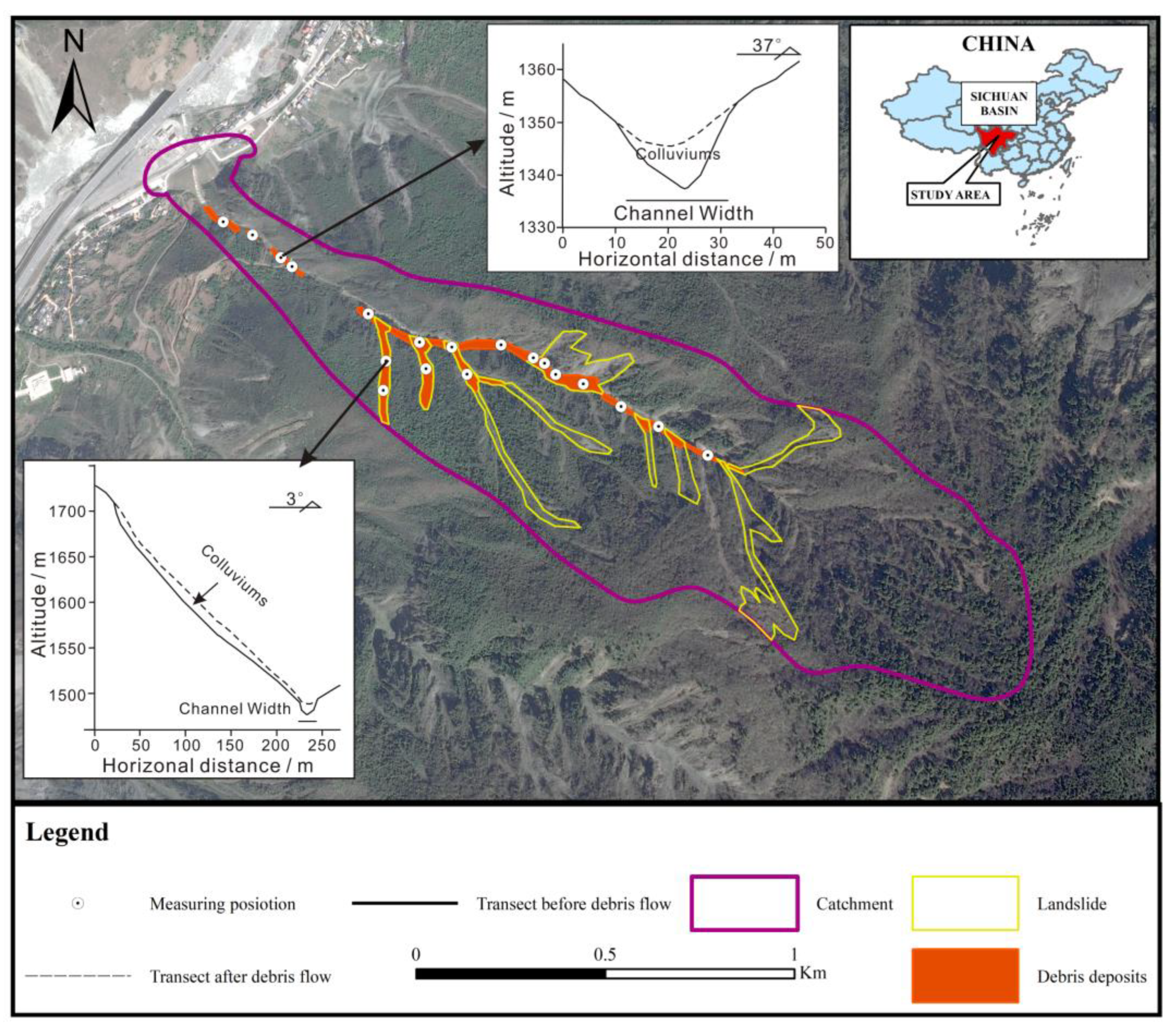
The Wayao catchment is located in Gaodian, Sichuan, China (
Figure 1). It is located in the Longmen Shan range, a region between the Qinghai-Tibet Plateau and the Sichuan Basin [
38,
39]. The catchment area is 11.7 km
2, and the main channel length is 2.2 km. The terrain elevation varies between 1191 m and 2973 m, and the slope range is 35–50°. The geological setting consists mostly of Proterozoic magmatic rocks. The Wayao catchment is located southeast of the Wenchuan-Maoxian fault, a thrust fault with a strike of 25° N–45° E [
40] that ruptured in the Wenchuan earthquake [
41]. Several landslides were triggered by the 2008 Wenchuan earthquake in the Wayao catchment, and most of them were deposited on the slope or along the channel. They provided the main debris source for the debris flow in 2013. The Wayao catchment is in a typically humid subtropical monsoon climate zone, with rainfall mainly concentrated between June and September. Heavy rainfall triggered two debris flow events in the Wayao catchment in 2013 and 2019.
On 10 July 2013, a catastrophic debris flow triggered by heavy rainfall destroyed the village located in the Wayao catchment outlet (
Figure 2). The triggering rainfall of the debris flow was 18.6 mm/h at 9 a.m. on 10 July 2013. The rainfall data are from a rain gauge approximately 9 km from the study area [
42]. The debris flow was triggered by the channel runoff, and several landslides were triggered by heavy rainfall [
43]. The deposition in the channel and several landslides along the channel provided source material for the debris flow. The debris flow eroded the deposited debris along the channel and stopped at the mouth of the catchment. Approximately 1.41 × 10
5 m
3 of debris was transported out, and the average depth of the debris fan was 5 m. The debris flow buried 27 houses and cut national road G213. Then, the local government built a check dam and drainage channel in 2014 to avoid possible debris flows.
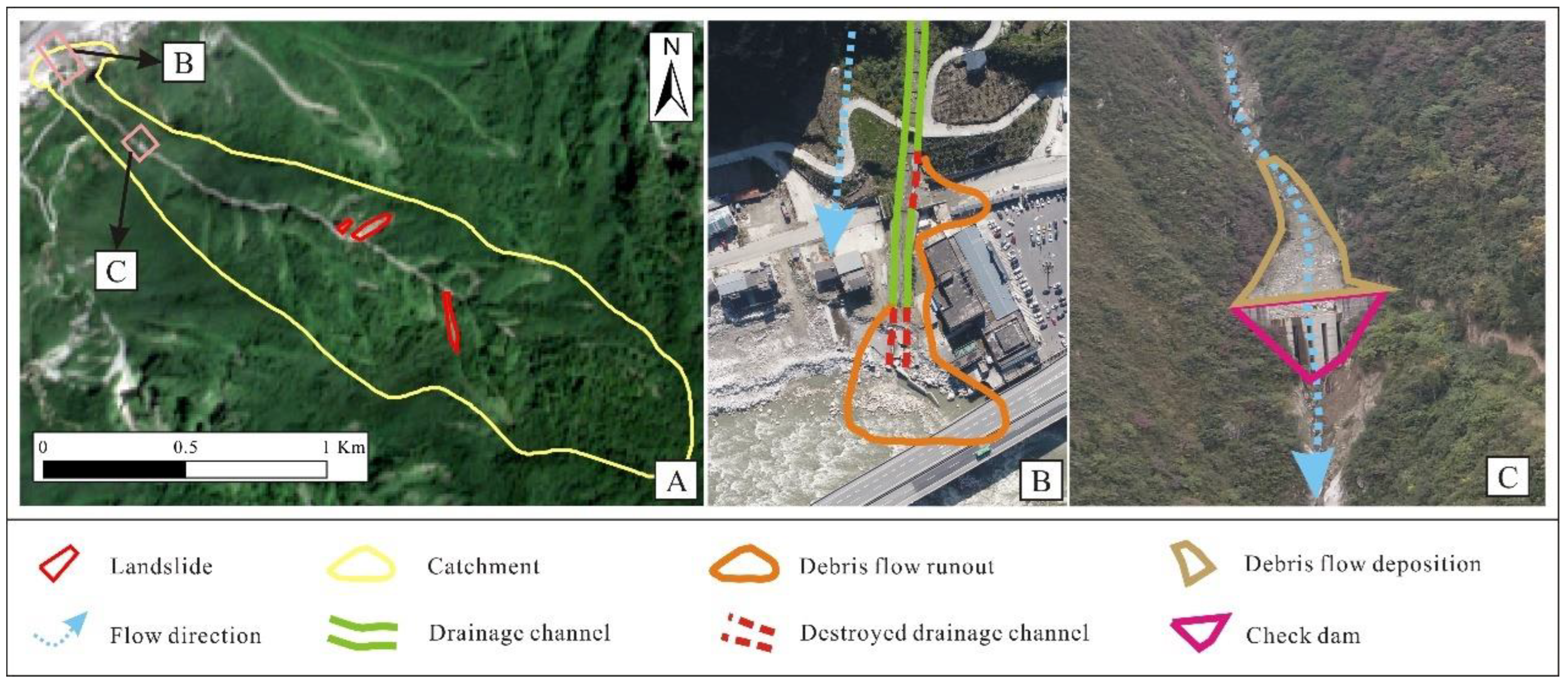
On 17 August 2020, during a rainstorm, the Wayao catchment suffered from a debris flow. The triggering rainfall of the debris flow was 18.8 mm/h at 4 p.m. The rainfall data are from a rain gauge about 18 km from the catchment and provided by the Sichuan Provincial Meteorological Service. The debris flow was triggered by the channel runoff, and three landslides were triggered by heavy rainfall. The three landslides provided the main source material for the debris flow, and some of the deposition along the channel was eroded by the debris flow. When the debris flow was transported to the check dam, the check dam was filled by the debris flow deposition. Then the debris flow was transported along the drainage channel, and most of the debris flow was transported into the Min River (
Figure 3).
3. Measuring Debris Flow Volume
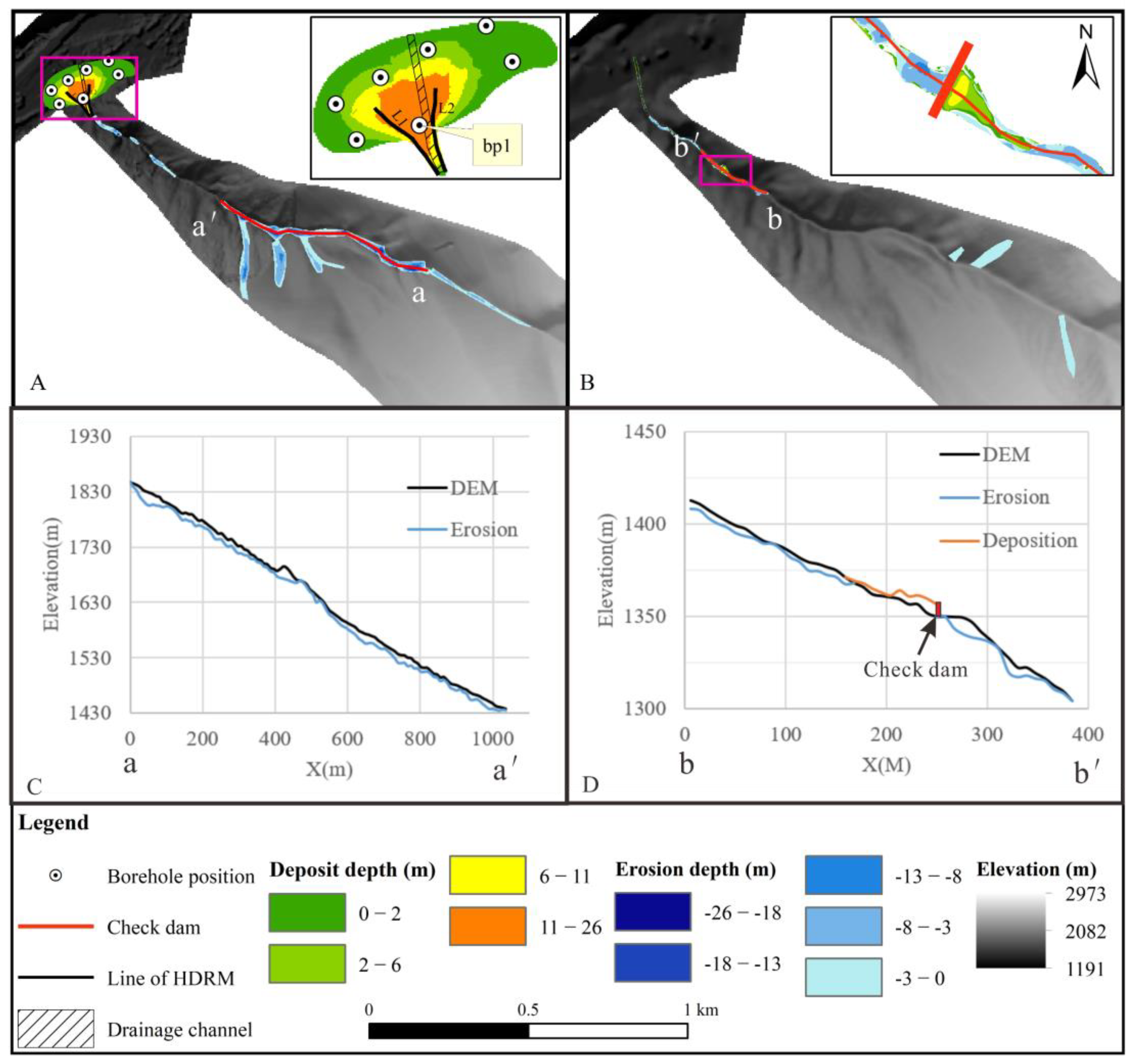
The depth distribution of landslides, deposition along the channel, and the debris fan were measured by multiple methods. The volumes of landslides and deposits along the channel are important input parameters of the debris flow simulation. Moreover, the depth distribution of the debris fan is an important factor to evaluate the simulation results.
For the debris flow event in 2013, the locations of landslides were mapped by visual interpretation [
44] using the image from Google Earth taken on 15 April 2015, and the depths of landslides were measured by field measurement. The depth distribution of debris fan, landslides, and eroded debris along the channel is shown in
Figure 4A, and the volumes are shown in
Table 1. Eight sections along the channel and ten sections on the slope were measured. The depth distributions of landslides and deposits along the channel in 2013 are shown in
Figure 3A. The depth distribution of the debris fan was measured by electrical resistivity tomography (ERT). ERT is widely used to delineate the contact surface between the debris fan and the underlying rock layer [
45,
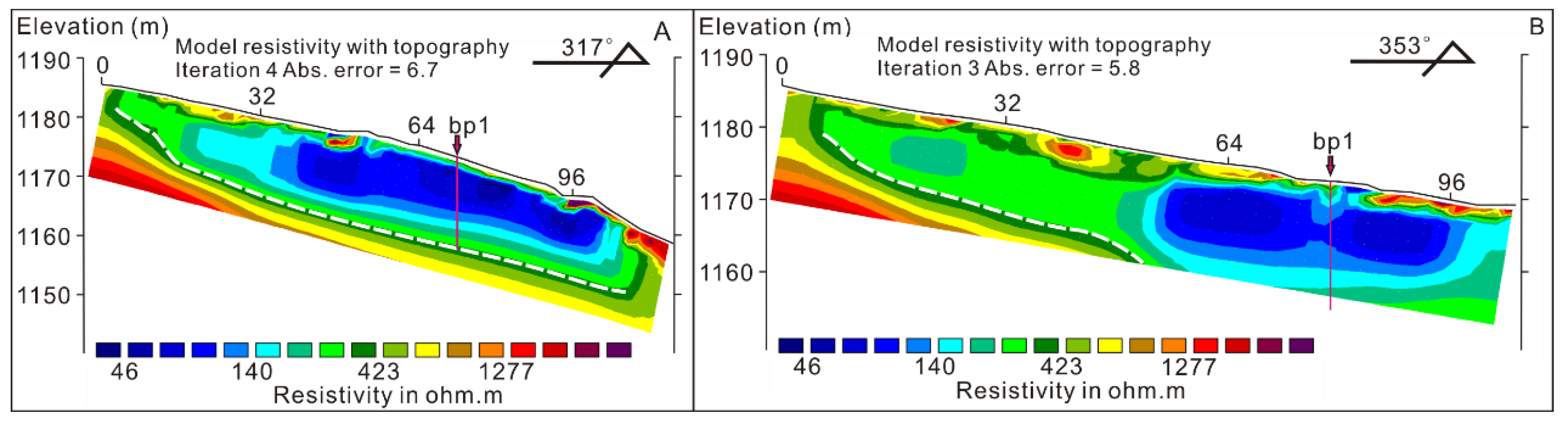
46]. ERT measurements were carried out on the deposition fan, and the instrument was a WDJD-3 system from Chongqing Benteng Digital Control Technical Institute. L1 and L2 were two measuring lines on the deposition fan (
Figure 4A). Sixty electrodes were placed on measuring line L1, and the distance between the electrodes was 2 m.
The total length of the L1 was 118 m. Fifty-four electrodes were placed on measuring line L2, and the distance between the electrodes was 2 m. The total length of L2 was 106 m. Res2DInv software was used for mesh refinement and robust inversion, and
Figure 5 shows the resistivity inversion results. At depths of 2 to 14 m, the electrical resistivity ranges from 40 to 200 Ω·m. At depths of 14 to 16 m, the values suddenly increase to 700–1000 Ω·m. The depth value of the debris fan is consistent with the value obtained by drilling (bp1). The location of bp1 was between the two measuring lines. Kriging [
47] was used to interpolate the depth values obtained by ERT and drilling. A 1:2000 topographic map, provided by the Sichuan Metallurgical and Geological Exploration Bureau of the Chengdu Geological Survey Institute, was used to build the terrain model for simulation of the debris flow in 2013.
For the debris flow event in 2020, the image from Sentinel-2 taken on 25 October 2020 was used to interpret the locations of rainfall-triggered landslides. Field measurements and UAV surveys measured the depths of landslides, eroded debris along the channel, and the deposition after the barrier. Their depth distributions are shown in
Figure 4B. Their volumes are shown in
Table 1. Two UAV stereo photo-derived digital elevation models (DEMs) were measured on 19 April 2019, and 25 October 2020. They are used to analyze the depth distribution of deposits along the channel by comparing. The DEM, measured on 19 April 2019, was used to build the terrain model for simulation of the debris flow in 2020.
4. Model Description
Four different models, Massflow, Flow-3D, OpenLISEM_A, and OpenLISEM_B, were used to simulate. They all require an input file of the debris volume in the release area. For Massflow and Flow-3D, the debris flow was assumed as a single-phase fluid, and the initial density of debris flow was measured by field survey. For OpenLISEM_A and OpenLISEM_B, the debris flow was assumed as a two-phase fluid mixed with fluid and solid. For OpenLISEM_A, the initial volume ratios of solid and liquid can be inversely calculated by debris flow density. For OpenLISEM_B, the input data was the debris source triggered by the rainfall. The debris source’s initial porosity and moisture content were measured by the field survey provided by the Sichuan Metallurgical and Geological Exploration Bureau of the Chengdu Geological Survey Institute.
They have different boundary conditions. For Massflow, OpenLISEM_A, and OpenLISEM_B, a hydrograph can be specified as boundary conditions. For Flow-3D, an outflow boundary condition was set to allow debris flow to continue through the boundary with minimal reflection [
25]. A man-made structure can be input into the four models, and the effort can be included in the simulation.
4.1. Massflow
Massflow is a program that adopts a depth-integrated continuum method to analyze the debris flow progress. It obtained good Hongchun debris flow simulation results in Wenchuan County [
17,
48]. For debris flow simulation, Massflow uses the Voellmy rheology. The Voellmy rheology assumes no shear deformation, and the mean velocity (
u) over the height of the flow (
h) of the flow is the same. The basal friction stress
τ is given by:
where
φ is the terrain’s downslope angle (positive),
μ is the dry Coulomb-type friction.
ξ is the viscous resistance. Massflow uses the MacCormack-TVD scheme to solve the shallow water equations [
17,
49].
The input parameters of Massflow are the depth distribution of debris flow, the resistance parameters
μ, and
ξ. For the simulation, the resolution of 5 m grid post-event topography data was adopted, and the data of the debris fan was replaced with the topographic map taken before the event. The dry friction factor was calculated as the surface slope of the debris fan, and its value was in a range between 0.4 and 0.45. According to past research, the viscous resistance was chosen in a range between 100 and 300 m/s
2 [
50,
51]. Then the inversion method was used to determine the specific parameter values. A series of numerical simulations were performed to refine the parameter values by comparing the depth distribution of the debris fan. Parameter values for Massflow are summarized in
Table 2. The running time was 300 s, with a time step Δt ≤ 1 s.
4.2. Flow-3D
Flow-3D is a general-purpose computational fluid dynamic (CFD) program. For debris flow simulation, Flow-3D uses the high concentration granular model. The designation of high concentration granular flow here means the volume fraction of the granular material is 50% or greater. A strong coupling exists between the solid particles and surrounding fluid at high concentrations, so their mixture can be approximated as a single composite fluid [
25]. The shear stress in non-cohesive granular flow consists of three parts: Impact among solid particles
τi, additional viscous shear stress due to the presence of solid particles
τv, and Shear stress in the fluid
τf.
where
μf is the fluid’s dynamic viscosity.
λ is the diameter to the minimum gap ratio. du/dy is the velocity gradient of the mixture.
ρs is the density of the solid sphere.
ρf is the density of the fluid sphere.
e is the coefficient of restitution of the solid particle, and a typical coefficient of restitution for debris of 0.7 is assumed as a good general value.
D is the diameter of spherical particles. Δ
R is the gap of a Couette flow.
λ is a function of the maximum solid volume fraction
divided by the solid volume fraction
fs.
when the volume fraction of solid material reaches or exceeds a value of about 0.99
, the flow velocity is set to zero, and the material is considered to be fully packed. A typical close packing volume fraction
for debris of 0.68 and the typical value of loose packing volume fraction for debris
of 0.11 are assumed as good general values. As granular material packs to a density where individual grains begin to touch one another, it becomes more difficult for the mixture to flow. This state is sometimes referred to as mechanical jamming and has a typical volume fraction of
= 0.62.
The simulation area at the Wayao catchment includes the debris source and the deposition fan areas. The terrain model was resampled with a 5-m triangular mesh, and it contains more than 996,000 facets. The landslide and deposit along the channel models were resampled with a 2-m triangular mesh containing more than 63,000 facets. According to the field survey, the density and viscosity of the fluid were set to 1000 kg/m
3 and 0.01 kg/m/s, respectively. The density of the solid was set to 2700 kg/m
3. The average grain diameter was set to 0.05 m, which was calculated by the measured value of the final deposit [
18]. The friction angle (degrees) was between 20 and ~35, as provided by the Sichuan Metallurgical and Geological Exploration Bureau of the Chengdu Geological Survey Institute. The debris flow density was in a range between 1850 and 2030 kg/m
3. The best simulation parameters were obtained through repeated analysis, and the simulation results were satisfactory.
Table 2 shows the full set of parameters used in the simulation. The running time was 300 s, with a time step Δt ≤ 0.5 s.
4.3. OpenLISEM_A and OpenLISEM_B
OpenLISEM is a physically based numerical program for simulating flood, erosion, and debris flow [
37]. It is based on the two-phase debris flow equations [
33] and a full hydrological catchment model that includes pressure, gravitational forces, viscous forces, non-Newtonian viscosity, two-phase drag, and a Mohr–Coulomb type friction force. It can simulate the flow dynamics and interactions of the flood and the nonuniform debris flow [
37,
52]. The following is a constitutive equation:
where α
s is the volume fraction of solid phases (-), α
f is the volume fraction of fluid phases (-). δ is the internal friction angle. P
b is the pressure at the surface (Kg/ms
2). b is the basal surface of the flow (m). N
R is the Reynolds number (-). N
RA is the quasi-Reynolds number (-). C
DG is the drag coefficient (-).
ρf is the density of the fluid (kg/m
3),
ρs is the density of the solids (kg/m
3), γ is the density ratio between the fluid and solid phase (-). χ is the vertical shearing of fluid velocity (m/s). ε is the aspect ratio of the model (-).
ξ is the vertical distribution of α
s (m
−1).
We performed two kinds of simulations using the OpenLISEM model. First, we applied a model that does not include the interception model (OpenLISEM_A), and it is the same as Massflow and Flow-3D, which ignore the initiation process of debris flow. According to the field survey, the solid’s density was set to 2700 kg/m
3. The friction angle (degrees) was in a range between 20 and ~35. The debris flow density was in a range between 1850 and 2030 kg/m
3. The value of manning was between 0.02 and 0.1. The porosity was set to 0.38. According to the research results [
17], the cohesion was in a range between 0 and 2500 pa.
Second, we ran a model that includes the interception and slope failure models (OpenLISEM_B). It is used to analyze the influence of rainfall conditions on debris flow prediction. In OpenLISEM_B, the slope failure and debris flow runout would be triggered by rainfall. According to the field survey, the value of the initial moisture content of the debris source is set to 0.114, and the rainfall was set to 18.6 mm/h. The debris flow density would change dynamically with rainfall.
A series of numerical simulations were performed to refine the parameter values by comparing the depth distribution of the debris fan. Parameters values for OpenLISEM_A and OpenLISEM_B are summarized in
Table 2. Both models were run for 15 min of real-event duration, with a time step constrained to ∆t ≤ 1 s.
5. Results
5.1. Application to the Debris Flow Event in 2013
The debris fan’s depth distribution was used to test the numerical parameters in four models.
Table 3 shows the analysis of the dependence of the final deposition volume in the debris fan area on the various parameters.
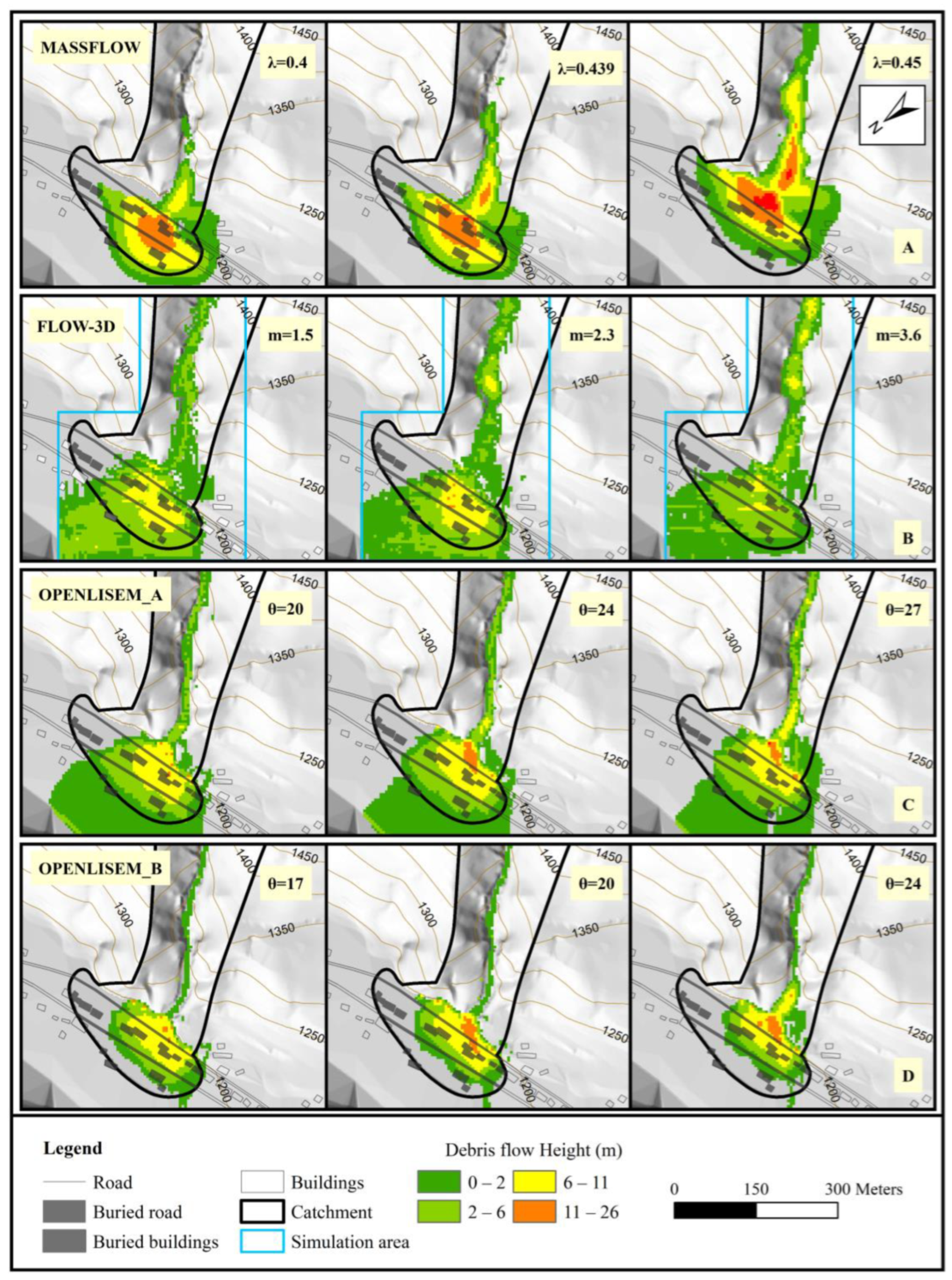
Figure 6 shows the four models’ simulation results with different numerical parameters.
For the Massflow simulations, we found that the final debris fan volume is sensitive to the Coulomb-type friction (
μ) and viscous resistance (
ξ).
Figure 6A shows the geometry of the debris fan with several different choices for the Coulomb-type friction (
μ = 0.4, 0.439, and 0.45). The simulation results show that the extent of the debris fan tends to be smaller than that of the real debris fan. However, Massflow reproduces the thickness distribution of debris deposition. Only the western part of the actual debris fan is slightly overestimated, and the eastern part is slightly underestimated. The simulation result with
μ = 0.439 is considered to best reproduce the debris flow deposition, and the volume of the simulated debris fan is 85% of the actual debris fan volume. However, this would lead to the selection of a very low friction angle, and this situation is the same as that found in Scaringi et al. [
53].
For the Flow-3D model, we found that the debris fan volume is more sensitive to the debris density and the friction angle. When the value of debris flow density is 2030 kg/m3, most of the debris flow deposits in the channel. When the value of debris flow density is 1850 kg/ m3, most of the debris flow runs out of the catchment at an abnormal velocity. The friction angle (θ) is another key parameter to the deposition and entrainment of the debris flow. A larger friction angle will cause the debris flow to deposit quickly, while a smaller friction angle will cause the solid particles to be more easily transported. Different simulations were performed to understand the friction angle (θ) influence on the debris flow process. We found that the multiplier in the friction angle significantly impacts the deposition rate of debris flow. The simulation result with θ = 32 is considered to best reproduce the debris flow deposition, and the volume of the simulated debris fan is 67% of the actual debris fan volume. However, the deposition thicknesses in the middle and east of the debris fan are underestimated.
For OpenLISEM_A, we found that debris fan volume is more sensitive to debris flow density, manning, and friction angle (θ), while less sensitive to cohesion. When the value of the friction angle was 20 degrees, most of the debris flow ran out of the catchment at an abnormal velocity. When the value of the friction angle is larger than 30 degrees, the velocity of debris flow will decrease significantly as the internal friction angle increase. The simulation results show that the extent of the debris fan tends to be larger than that of the real debris fan, and the deposit thickness in the east of the debris fan is underestimated (
Figure 6C). The simulation with θ = 24 is considered to best reproduce the debris flow deposition, and the volume of the simulated debris fan is 73% of the actual debris fan volume.
For OpenLISEM_B, we found that debris fan volume is more sensitive to manning and the friction angle (θ) while less sensitive to cohesion. The influence on the debris flow behavior of the friction angle was similar to that in OpenLISEM_A. However, the simulation result with θ = 20 is considered to reproduce the debris flow deposition best, and the value is smaller than that of OpenLISEM_A. The failure volume of the slope is determined based on the infinite slope method. The failure part may slide into the channel and participate in the debris flow.
Figure 6D shows that the extent of the debris fan tends to be smaller than the real extent, and the thickness distribution of debris deposition is also underestimated. The simulation with θ = 20 is considered to best reproduce the debris flow deposition, and the volume of the simulated debris fan is 59% of the actual debris fan volume. The extent and volume of the debris fan in OpenLISEM_B is smaller than that in OpenLISEM_A. It is speculated that part of the debris source was transported out of the debris fan extent by the channel flood under the rainfall condition.
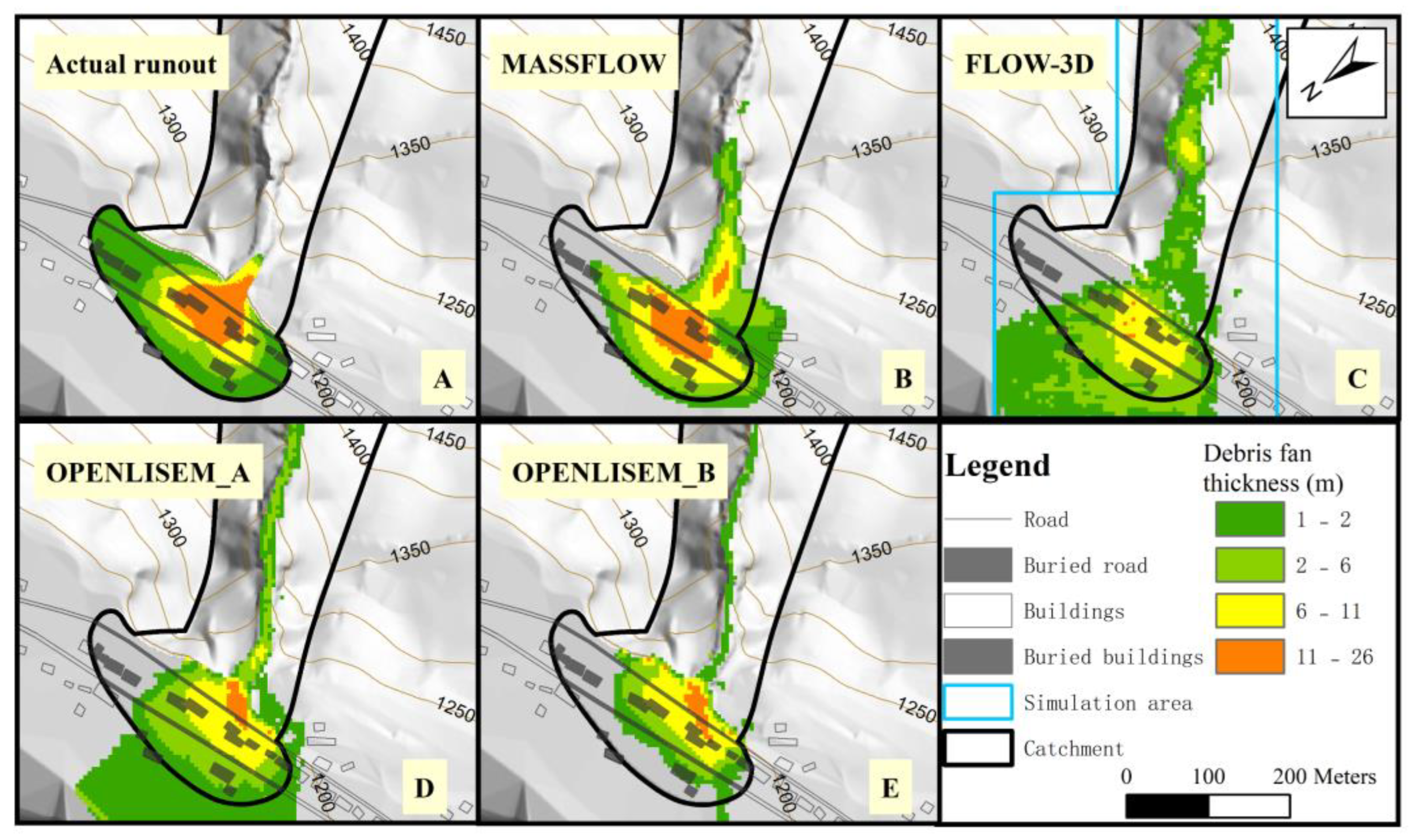
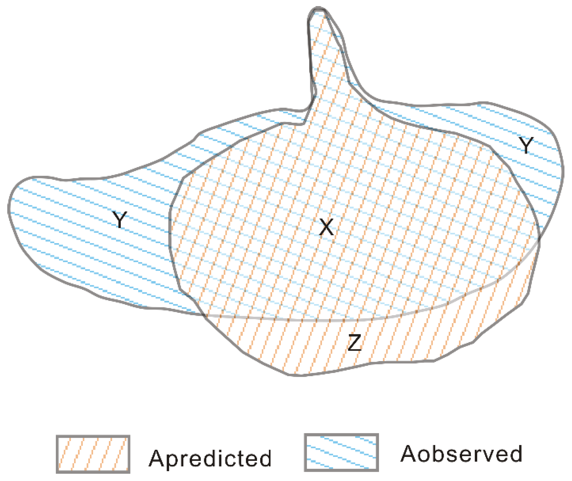
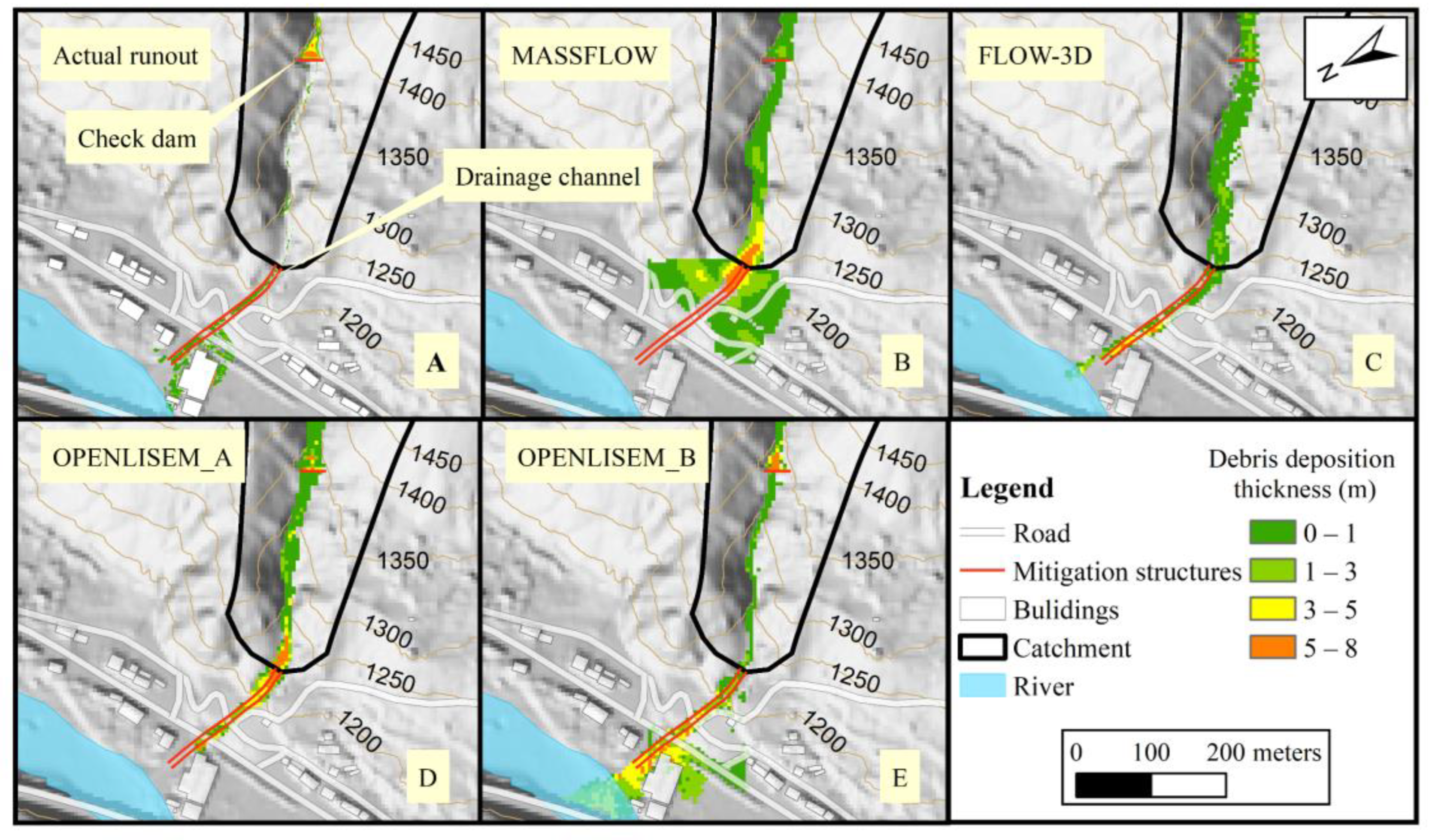
The four models can reproduce the geometry and thickness distribution of the debris flow fan (
Figure 7). The schematic diagram of verification results is shown in
Figure 8, and the accuracy [
9] of the four models is shown in
Table 4. The Massflow and OpenLISEM_A models seem to reproduce the actual deposit area and volume more accurately than other models. The positive accuracy area of Massflow and OpenLISEM_A was higher than 70%, and the positive accuracy volume of Massflow (86%) was the best of all. The positive accuracy area and volume of Flow-3D were lower than 70%. Flow-3D shows a runout spread of debris flow larger than that in the actual event, and the negative accuracy area of Flow-3D was 73%. OpenLISEM_B shows a runout spread of debris flows smaller than that in the actual event. The positive accuracy area and volume of OpenLISEM_B were lower than 60%, but the negative accuracy area was the smallest. All models underestimate the eastern part of the debris fan, which was discussed in
Section 6.
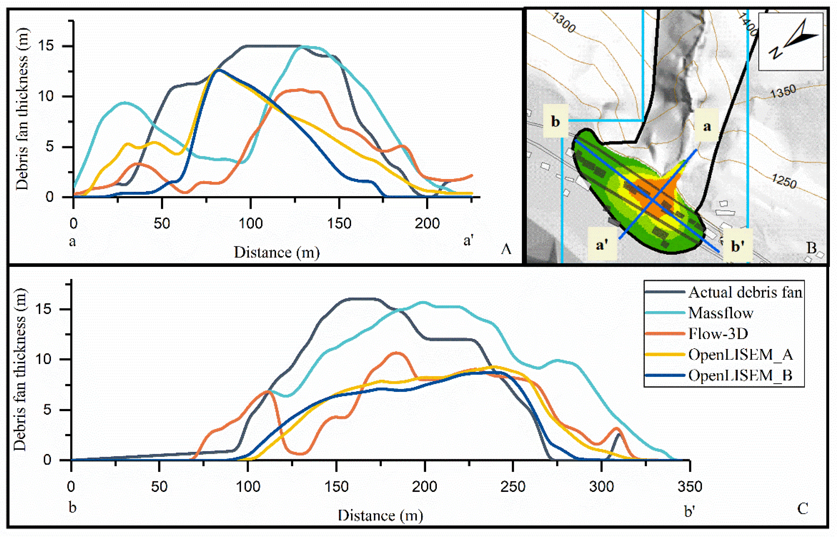
The thickness of the debris fan in the best-fit simulations of various models was compared (
Figure 9). Massflow and Flow-3D present the same thickness distribution in section a-a’. The thickness values of Massflow are closer to the actual values than Flow-3D. Those values are approximately 5 m larger than that of Flow-3D. OpenLISEM_A and OpenLISEM_B present almost the same thickness distribution in two sections as they use the same debris flow equations. The depth distribution of Massflow in section b-b’ is closer to the actual depth distribution than the other three models. Massflow presents the same thickness distribution shape as reality, and only the peak value is shifted. Flow-3D, OpenLISEM_A, and OpenLISEM_B have similar thickness distributions of debris fan, and they all underestimate the thickness distribution at 100–250 m (
Figure 9C).
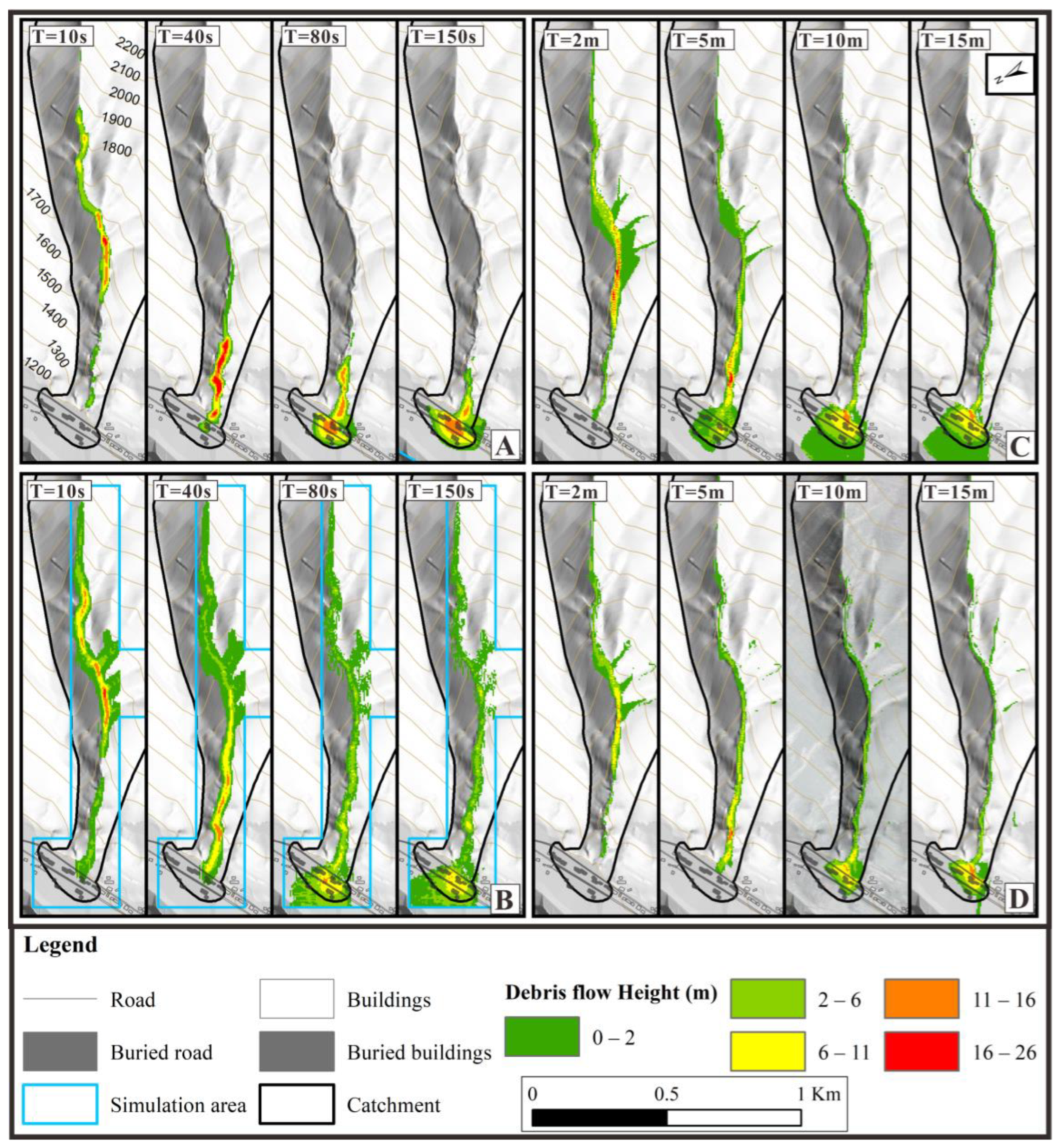
The depth distribution of the debris flow at four representative moments after the initiation of the debris flow was compared (
Figure 10). Despite the different modeling methods, the depth distributions resulting from the Massflow and Flow-3D simulations are very similar in terms of runouts versus time and the spatial distribution of depth at each moment. Due to the different resistance terms of debris flows in the models, the flow velocities of debris flow in Massflow and Flow-3D simulations are significantly higher than OpenLISEM_A and OpenLISEM_B. Compared with OpenLISEM_B, OpenLISEM_A does not include the hydrological model, so the processes of rainfall infiltration and slope failure were omitted. Therefore, the time for the debris flow to reach the catchment mouth in OpenLISEM_A is less than that in OpenLISEM_B (
Figure 10C,D).
5.2. Prediction to the Debris Flow Event in 2020
To evaluate the prediction ability of the four models for possible debris flows, we use the simulation results of the Wayao debris flow event in 2020. The sets of parameters for prediction were the same as those for the Wayao debris flow in 2013 simulations. The depth distribution of the debris flow in 2020 was created as the input file. The rainfall value was 18.8 mm/h in 2020. The depth distribution verified the prediction ability of different models.
The simulation results of the four models are shown in
Figure 11 to compare the runout areas of different models. According to the UAV survey, the debris flow filled the check dam in 2020, and the max depth value of the deposition was 7.6 m. Most of the debris flow ran into the Min River, and only a few were deposited along the channel.
For Massflow, the simulation result shows that the runout extent of the debris flow was more significant than the real in 2020. Some of the debris flow was deposited after the check dam, and the max depth of the deposition was 1.9 m. Most of the debris flow deposits at the junction of the catchment channel and the drainage channel, and the max deposition depth was 8.3 m.
For Flow-3D, the simulation result shows that most of the debris flow ran into the Min River which is consistent with reality. The deposition depth in the drainage channel was slightly overestimated, and the value range was between 0.2 and 4.3 m. The deposition depth after the check dam was underestimated, and the max value of depth was 2.2 m.
For OpenLISEM_A, the simulation result shows debris flow transported along the drainage channel. However, most of the debris flow was deposited at the junction of the catchment channel and the drainage channel, and the max depth of deposition was 5.6 m. The deposition depth after the check dam was underestimated, and the max value of depth was 3.6 m.
Among all the models, OpenLISEM_B yields the result most consistent with the actual situation. The simulation and the actual error are approximately 25% at the deposition depth and volume behind the dam. Most debris flows ran into the Min River along the drainage channel. A small part of the debris flow was deposited in the drainage channel, and the depth was approximately 0.5–1.1 m.
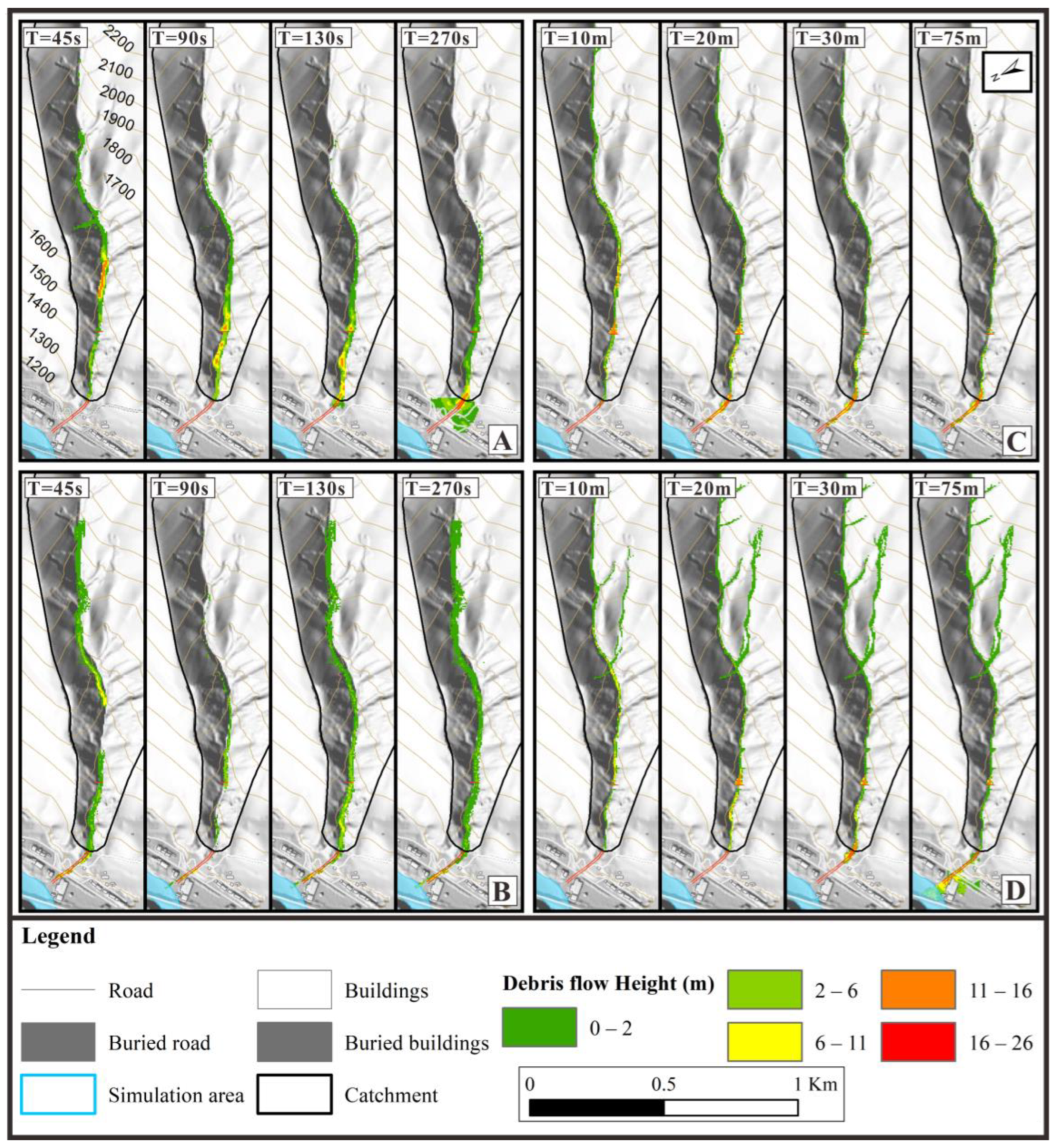
Figure 12 shows the comparison of the depth distribution of the debris flow at four representative moments after the initiation of the debris flow. The simulation results of Massflow and Flow-3D show that the time when debris flow reaches the mouth of the catchment is approximately 3 min. The time for OpenLISEM_A and OpenLISEM_B is approximately 20~30 min. For Massflow and OpenLISEM_A, the debris flow deposited along the channel in the simulation results. For Flow-3D and OpenLISEM_B, most of the debris flow ran into the Min River in the simulation result. The comparison between OpenLISEM_A and OpenLISEM_B indicates that when the debris flow arrives at the channel with a gentle slope, the channel flow formed by rainfall could provide momentum for the debris flow. If the debris flow model does not include the hydrological model, the debris flow would rapidly deposit along the channel with a gentle slope.
5.3. Scenario without Mitigation Structures
We evaluated the impacts of mitigation structures on the uncertainty of predication with the depth distribution of debris flow deposition. The four models were used to predict without mitigation structures. The simulation parameters were the same as those in
Section 5.2, and the mitigation structures were taken out from the models.
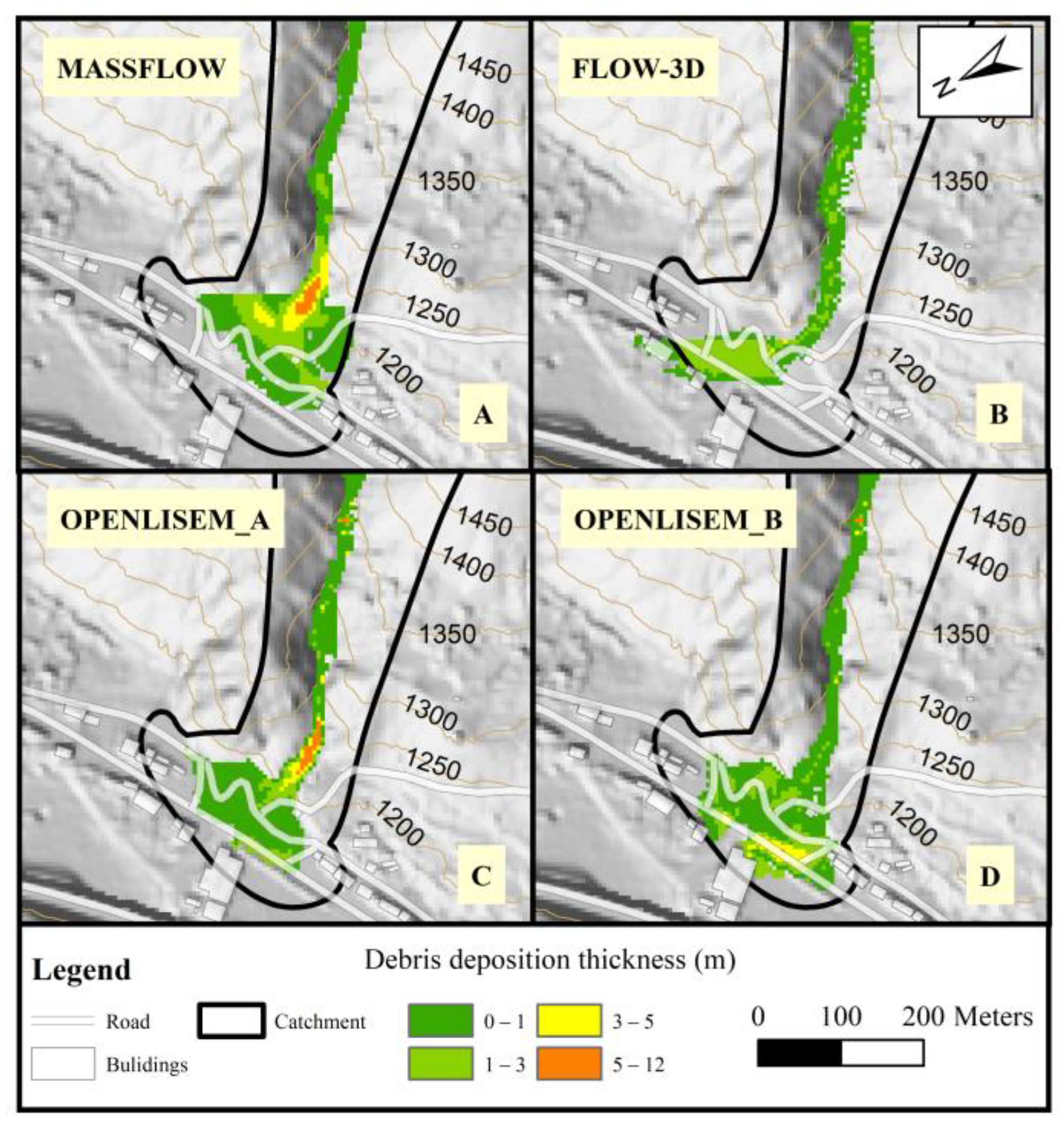
Figure 13 shows the prediction results of the four models. The simulation results show that the debris flow ran out of the catchment. However, the depth distributions of the debris flow deposition were different.
For Massflow and OpenLISEM_A, most of the debris flow was deposited at the mouth of the catchment, and the main deposit area was along the channel. This result indicates that the structures had limited effort on the deposition progress of debris flow in
Figure 12.
For Flow-3D, OpenLISEM_A, and OpenLISEM_B, the simulation results show that the extent of runout areas was more significant than that in
Figure 12. The debris flow buried part of the road and several houses. The simulation result for Flow-3D shows that the main threat area was located east of the catchment mouth. The debris flow buried five houses and part of the roads. However, the west area of the catchment mouth was safe. This result indicates that the mitigation structures played an essential role in reducing the danger of the debris flow event in 2020.
The results of debris-flow risk assessment have important guiding significance for land planning and the construction of prevention and control projects in mountainous areas. When selecting debris-flow risk assessment models, each model’s advantages and disadvantages should be thoroughly evaluated. A simulation model suitable for the study area should be selected. Alternatively, a multi-model combination method should be adopted.
6. Discussion
Table 2 shows that the value of friction angle in the different models is significantly different. The models assume that the parameters of debris flow are constant. However, they are not evenly distributed in all catchments, such as particle size and internal friction Angle. The parameters values obtained by the field survey are in a range. The parameter values in
Table 2 are optimal simulation values, and they were obtained by parameter correction.
Figure 8 shows that all models underestimated the eastern part of the debris fan in 2013. According to reports from villagers who witnessed the debris flow, the Wayao debris flow ran out several times on 10 July 2013. Moreover, we infer that numerous debris flows formed the deposits in the eastern part of the debris fan. The phenomenon is related to rainfall scenarios, random rainfall-triggered landslides [
54], natural debris dams in the channel, and natural dam failure [
55].
The hydrological condition is one of the critical parameters in debris-flow simulation. There is interaction or feedback between the hydrology and a debris flow. When this interaction is not considered in the model, the model’s predictive power is limited [
37]. As we can see in
Section 5.2, the debris flows in the simulation results for OpenLISEM_A stopped at the drainage channel. However, most of the debris flow in the simulation result for OpenLISEM_B ran into the Min River. According to Equations (4)–(7), for OpenLISEM_A, the initial volume fraction for solid and fluid phases is constant. However, for OpenLISEM_B, the two values change dynamically with rainfall, and this is an important reason why the prediction result of OpenLISEM_B is better than that of OpenLISEM_A.
In the Massflow prediction results, the runout distance of debris flow was underestimated. According to the dependence analysis, the value of the Coulomb-type friction is proportional to the runout distance of debris flow. In Equation (1), the value of the Coulomb-type friction is proportional to the basal friction stress. Therefore, we believe that the value of the Coulomb-type friction was underestimated in the debris flow simulation in 2020.
The quantity and accuracy of rainfall data affect the simulation results, as OpenLISEM_B is sensitive to rainfall. In mountainous areas, precipitation may vary significantly in space [
56,
57]. The uncertainty error between the measured and actual rainfall values is a limitation of this manuscript, although we have obtained acceptable measured results by parameter calibration.
In some cases, parameter calibration can obtain satisfactory results, such as the simulation results in
Section 5.1. However, the simulation accuracy may be significantly reduced when these parameters are applied to debris flow prediction. None of the models used in this work can be considered superior to the others. Discrimination among models should also evaluate the actual usability of the model and its results. For example, a model should be assessed in terms of the ease of use, the quantitative and physical significance of the parameter assessment or calibration, the possibility of incorporating the model into early warning systems [
58,
59], and finally, the calculation time. In the case of incorporating the model into a real-time risk assessment system, the last factor may be decisive since the inputs to the model may change over time, and the new solutions must be recalculated in time to alert. On the other hand, in the situations that the imminent failure is not expected or detailed risk assessment in land use is required, priority should be given to the accuracy of debris flow prediction. It needs to combine more field surveys and experiments to obtain physical parameters, and reproduce the complex debris flow process.
If the computation time is considered unique (
Table 5), not including the modeling time, Massflow can simulate the entire debris flow process in less than 5 min. A desktop computer (CPU, AMD 2700X, 16 cores, 3.7 GHz; RAM, 16 G) was used, and the resolution terrain grid was 5-m. When the same simulation is performed on a 10-m resolution grid, Flow-3D takes 14 min. At the same time, the calculation on a 5-m grid takes approximately 2 h. Of course, the performance of Flow-3D models can be significantly improved by using multicore/parallel solvers to run the code on a powerful workstation [
25]. OpenLISEM_A takes approximately half an hour on the same machine, but with a less precise (10 m) grid, the time is cut in half. However, the simulation time of OpenLISEM_B with the hydrological model is much longer. The time for 10 m resolution exceeds one hour, while the 5 m resolution requires more than two hours.
The topographic mesh resolution affects the time for computation and the simulation result. So, the appropriate resolution requires consideration of both computational efficiency and debris flow progresses [
60]. For Massflow and Flow-3D, the simulation results on the 5-m grid and the 10-m grid were similar. However, for OpenLISEM_A and OpenLISEM_B, the grid size significantly influenced the debris flow height and velocity and this is the consistent result of Bout and Jetten [
52]’s sensitivity test on terrain resolution.
The advantages of Massflow are its simple parameter requirements and high computational efficiency, and the data can be directly exported through a geographical information system (GIS). When the accuracy of the debris flow deposition range is not high, preliminary hazard prediction can be made by Massflow. OpenLISEM requires more parameters than the other two models, but GIS can also integrate input parameters. Flow-3D has the most parameters, and its terrain model needs to utilize professional modeling software, so there may be some difficulties in operation. However, a three-dimensional description of the structure of prevention measures can be realized, which is a significant advantage in evaluating debris flow prevention projects for the future.
A common shortcoming of the simple-phase models used is that the initial spatial distribution of the simplified variables (e.g., porosity, saturation, and cohesion in the soil) cannot be easily considered. For example, the particle size distribution and the angle of internal friction in the debris source are single values for the entire catchment (
Table 1). Similarly, in two-phase models, the input of a material parameter is its spatial distribution. This input has important implications for hazard assessment using numerical methods and developing early warning systems to mitigate risks.
Finally, it is worth re-emphasizing predictions of future events.
Different models have different predictive capabilities, and this may be due to the different sensitivity to debris flow densities or considering the interactions between the hydrology and the debris flow. Therefore, it should be considered when evaluating model predictive reliability.
Adopting multiple methods in hazard assessment and early warning systems may achieve ideal results. For example, a model with higher computational efficiency is used for preliminary prediction. Moreover, a model with higher accuracy is used for detailed prediction.
It is unclear whether a model is always the best performance model for prediction. Therefore, combining various models to form a multi-model real-time risk assessment and early warning system requires further research.
7. Conclusions
In this work, two single-phase models (Massflow and Flow-3D) and two-phase flow models (OpenLISEM_A and OpenLISEM_B) were applied to reproduce the main movement and deposition characteristics of the Wayao debris flow event in 2013. Moreover, the four models were applied to predict the Wayao debris flow event in 2020, and the parameters are the same as those in 2013. The depth distribution of debris flow was used to analyze prediction accuracy. Some conclusions can be drawn:
All four models provided satisfactory results for the geometry and depth distribution of the debris fan in 2013.
Combining the simulation results in the scenario without mitigation structures indicates that the mitigation structures played an essential role in reducing the danger of the debris flow event in 2020.
Considering the prediction of the debris flow event in 2020, including the deposition depth of debris behind the check dam and the runout extent of the debris flow, OpenLISEM_B has the best performance among the four models. However, they are different for both the adopted theoretical rheological model and the numerical scheme. So, it is not easy to understand the different behavior.
OpenLISEM_B (the model with an entire hydrological catchment) has the advantage of higher prediction accuracy of debris flow deposition depth than OpenLISEM_A (the model without considering). Since the cases in this paper were triggered by runoff, the comparison can only stand for debris flows triggered by runoff.
While each model has its limitations, the simulation of possible future debris flows using back analysis of debris flow parameters based on existing debris flow events and field investigation of potential debris sources can be a helpful tool for local risk assessment. The ability to recalculate new solutions in a short time is necessary for a real-time early-warning system. The accuracy of model prediction under different rainfall scenarios is critical in hazard assessments of significant projects. Therefore, in different application scenarios, such as debris flow risk assessment or early warning systems, comprehensively consider the accuracy of the model prediction, the difficulty of parameter acquisition, and the computational time.


 ,
, 


