Low-Carbon Tour Route Algorithm of Urban Scenic Water Spots Based on an Improved DIANA Clustering Model

Abstract

Aiming at the problems in current research into low-carbon and water scenery tourism, this paper brings forward a low-carbon tour route algorithm of urban scenic water spots based on an improved Divisive Analysis clustering model. Based on the ecological attributes of scenic water spots, the clustering model is set up to create scenic spot clusters. Via the clusters, the low-carbon tour route algorithm of urban scenic water spots based on the optimal energy conservation and emission reduction mode is proposed, and it provides the optimal scenic water spots and low-carbon tour routes for tourists. The model can thus realize the optimization of vehicle exhaust emission in urban travel and reduce exhaust emission damage to urban water bodies and natural environments. In order to verify the advantages of the proposed algorithm, this paper performs an experiment to compare the proposed algorithm with the frequently used route planning methods by tourists. The experimental results show that the proposed algorithm has great advantages in energy conservation, emission reduction and low-carbon travel and can reduce the exhaust emission and the damage to the urban water bodies and the natural environment, realizing low-carbon tourism. The main findings and contributions of the proposed work are as follows. First, an improved clustering algorithm is set up, and the urban scenic water spots are clustered according to attribute data, which could optimize the scenic spot recommendation spatial model. Second, combining with the specific characteristics of scenic water spots, the scenic spot mining and matching algorithm is set up to satisfy tourists’ needs. Third, a method that could reduce emission exhaust by optimizing self-driving tour routes is proposed, which could control and reduce the damage to urban environments and protect water ecosystems. The proposed algorithm could be used as the embedded algorithm of tour recommendation systems or the reference algorithm for planning urban tourism transportation. Especially in peak tourism season, it could be used as an effective method for tourism and traffic management departments to direct traffic flow.

1. Introduction

In tourism projects, water scenery tourism is a very popular type. It is a collective name for tourism activities that rely on water resources in scenic spots. Water scenery tourism mainly relies on water resources; thus, scenic spots constructed on water not only have the function of providing sightseeing locations but also aim to maintain urban ecological environments, regulate water circulation, regulate the urban temperature and beautify the urban environment. Thus, it is necessary to protect urban scenic water spots [1]. Urban water scenery tourism resources are relatively scarce. People have hydrophilic psychology; thus, urban scenic water spots must not only have features of landscape design and sightseeing but also other features. Their multiple attributes determine that the urban scenic water spots can provide recreation and rest places and also provide other tourism functions, such as culture, sports, health, etc. In addition to these attributes, since scenic water spots are distributed in the city geospatial environment, they have geospatial features, namely spatial location, distance relation, water area, etc., which assigns them to the research category of tourism geographic information systems. Some scenic water spots are classical and popular ones, which not only attract local tourists but also attract a large number of out-of-town tourists [2]. When the vast majority of scenic spots in a city are scenic water spots, the city can be identified as a water tourism resource city. Urban water tourism resources should be reasonably developed and effectively protected. As an important component of ecosystems, the water cycle plays an important part in regulating the urban natural environment, in which scenic water spots play a key role [3]. Every year, tens of thousands of tourists come to visit these scenic spots, and their activities will impact the urban ecosystems. Under the condition of huge quantities of tourists, it is important to reduce exhaust emission and the damage to urban ecosystems while meeting tourists’ needs and finally to realize low-carbon travel [4,5,6].

Currently, the research on urban water scenery tourism and low-carbon tourism mainly focuses on the following aspects. The first is the development of the mode and mechanism of water scenery tourism or the products of water scenery tourism. The second is research on the spatial distribution of water tourism resources. The third is the present situation and mechanism of low-carbon tourism. Li [7] analyzed the problems associated with water tourism resources and proposed development prospects. This study mainly addressed existing problems in rural water tourism resources and proposed new ideas for optimizing spatial patterns, changing the mode of production and adjusting the industrial structure. Zhou [8] classified water tourism resources, used the AHP method to conduct an investigation on Zhangjiajie water tourism resources, and brought forward improvement suggestions. The study reached the following conclusions: Zhangjiajie’s water resources are abundant, but the overall quality is low. The main improvements should include water quality monitoring, developing new modes of water tourism and improving the basic transportation system. Xu [9] studied the usage and development of Chizhou city’s water tourism resources and found that that resource integration, brand building and increasing capital investment are necessary. Li [10] studied the development strategy of urban water ecotourism, identifying the issues with water tourism resources and the corresponding countermeasures. Cao [11] conducted statistical analysis of tourists’ cognition and studied urban water scenery tourism. Cao proposed the principles and ideas behind urban water tourism development, development methods for water tourism activities and purification methods for water environments. Fan [12] conducted data mining on the cultural attributes of water tourism resources in the process of tour planning. By mining the cultural attributes of the scenic water spots, Fan reached the conclusion that cultural attributes are indispensable factors for tourism activities. Li [13] studied the spatial distribution of water tourism resources in megacities and proposed an optimization method for water tourism spatial distribution. Li also determined the key issues that should be addressed in water tourism planning in the future. Song [14] conducted research on the products of water culture and reported the following conclusions: cultural attributes should be considered as critical concerns, and the role of cultural attributes should be emphasized in water tourism development. Dai [15] studied the development mode of water sports tourism, focusing on Hubei province, and proposed the possibility of further developing and promoting Hubei province water sports tourism. Huang [16] used the MCN mode to study the innovation in low-carbon tourism marketing and proposed innovative ideas for Heilongjiang province, including personnel training, establishing supply chains for low-carbon tourism and regulating marketing policies and systems. Tao [17] studied tourists’ low-carbon behaviors and came to the conclusion that the Harbin low-carbon tourism could be enhanced by increasing publicity, improving tourism facilities, improving public transportation networks, etc. Tian [18] conducted research on the feasibility and development of low-carbon tourism in Guilin and proposed strategies for promoting the construction of Guilin as a low-carbon tourism city. Wang [19] studied the intrinsic motivation of tourists’ low-carbon traveling activities and found that subjective norms, behavior attitudes and moral norms as well as knowledge of low-carbon options influence and drive low-carbon activities, while perceptual behavior control doesn’t have a significant impact. Ren [20] studied transformation strategies for low-carbon tourism in cities and proposed strategies for resource-exhausted cities to develop low-carbon tourism. Liu [21] conducted research on the construction and application of low-carbon tourism evaluation systems, determining the associated problems and proposing suggestions for improvement. The current studies on water scenery tourism and low-carbon tourism mainly focus on development modes, spatial distributions, low-carbon construction methods, etc., which have certain limitations. First, there has been no targeted research on the feature attributes of scenic water spots and their clustering modes. The clustering of scenic water spots is vital, since it is a precondition for low-carbon tour route research. Second, tourists’ behaviors when choosing scenic water spots in terms of the aspects of low carbon, lowest cost and the most benefits have not been studied. These are also preconditions for low-carbon tour route research, since identifying tourists’ needs is the key to realizing the lowest cost and the greatest benefits. Third, the optimization of the tour route via different transportation choices to ensure energy conservation and emissions reduction (ECER) has not been studied. The choice of transportation method is critical in low-carbon tourism research. When a majority of tourists choose optimal routes, it greatly reduces exhaust emissions. Aiming at the current problems and deficiencies of water scenery tourism, this paper proposes a low-carbon tour route algorithm for urban scenic water spots based on an improved DIANA clustering model. It mainly studies the optimization of scenic water tour routes in terms of scenic feature attributes, tourist choices of scenic spots, low-carbon tour route planning, etc. It aims to reduce exhaust emissions and help to protect urban ecosystems. Compared with the methods from the literature, the proposed algorithm focuses on quantitative study. Compared with [7], the research object of the proposed algorithm is urban water tourism resources, not rural water tourism resources. Urban water resources may be influenced by multiple factors and can be easily contaminated. Thus, they need specific strategies. Compared with [8], the proposed method involves an intensive quantitative study of tour routes and transportation modes and puts forward a specific algorithm. Compared with [9,10,11], the proposed method designs a specific algorithm for scenic water tour routes. It provides an optimized model of urban water tour routes based on geographic information and algorithm optimization. Compared with [12,13,14,15], the proposed method mines water tourism’s cultural attributes and sets them as labels to set up the algorithm. It is a concretization of the ideas presented in the literature. The literature [16,17,18,19,20,21] has analyzed the existing problems in the water tourism industry in terms of carbon imprint and has put forward optimization countermeasures and development paths for low-carbon tourism spatial optimization. Ref. [22] set up a mode of two-stage supply chain management to reduce greenhouse gases emissions. Ref. [23] proposed a closed-loop supply chain, which connects herbal medicine with biofuels. It can effectively increase waste utilization and reduce environmental pollution. Ref. [24] studied the different production strategies of two kinds of innovative green products and then developed three models to promote the reproduction of the innovative green products to realize environmental protection. Ref. [25] aimed to make pure biofuel with a smaller amount of carbon emission and energy utilization through a smart multi-type biofuel manufacturing framework. By using this method, the percentage of impure biofuel can be decreased through the minimized energy consumption. Compared with the literature [22,23,24,25], the proposed algorithm has a similar research idea, in which an optimization model is set up and the aim is to reduce greenhouse gas emissions. Refs. [22,23,24,25] mainly focused on biofuels, waste recycling, developing innovative green products and smart multi-type biofuel manufacturing, while the proposed algorithm reduces vehicle exhaust emission by optimizing tour routes and tourist activities.

The research objectives, innovations and novelties are as follows. First, aiming at the specific attributes of scenic water spots, this research proposes an improved DIANA algorithm, which generates scenic spot clusters on the basis of scenic water spot attributes. Thus, the clustering results are more accurate, conforming to tourists’ needs. Second, based on the clustering results, a tourist interest matching algorithm is set up to precisely mine the scenic water spots and enhance tourist satisfaction. Third, aiming at the issues surrounding low-carbon traveling, a low-carbon tour route planning algorithm based on search optimization is established, which can decrease exhaust emissions from self-driving vehicles to protect urban ecosystems and water resources.

2. Urban Scenic Water Spot Spatial Clustering Based on the Improved DIANA Algorithm

Urban scenic water spots have different feature attributes from other scenic spots. Their main bodies are water areas. They have the functions of sightseeing, recreation, culture transmission, and sports and health activities. When tourists choose the scenic water spots to visit, they usually have an intrinsic motivation related to their specific attributes, such as enjoying the scenery, boating, watching waterfowl, experiencing marine cultures and customs, swimming, diving, tasting seafood, etc. Tourists’ intrinsic motivations will directly determine the choice of scenic water spots. Usually, tourists’ intrinsic motivations match scenic water spots’ attributes [26,27].

According to their attributes, scenic water spots can be divided into several groups: recreation and sightseeing, boating, water culture and custom, and water sports. The recreation and sightseeing group includes all the leisure activities involved when visiting and viewing the water scenery and related supporting facilities. Boating includes sightseeing while on board a boat. The water culture and custom group involves appreciating the historical culture and customs of particular water areas. Water sports includes any physical sport played on, in or around water. Scenic water spots have four attributes: popularity degree, minimum cost, traveling time and spatial distance. The popularity degree is an average value that reflects tourists’ enthusiasm for a particular spot. The minimum cost is the lowest cost of visiting one scenic spot for one tourist (unit: ¥ yuan). The traveling time is the average suitable and comfortable leisure time that could be consumed in visiting one scenic spot (unit: hour). The spatial distance is the geospatial distance between one tour route’s starting point and one scenic spot, which is calculated by the longitude and latitude, and directly determines the traveling cost and exhaust emission. In the modeling of clustering and tour route planning, the groups and attributes should be quantified as a first step.

2.1. The Modeling of the Attribute Quantification Matrix for Scenic Water Spots

According to the principle of the clustering method, dots in space with the close attribute relationships can be classified into one cluster. The tour process is usually constrained by multiple factors. Thus, scenic spot recommendations should consider both classifications and attributes. The key to modeling the scenic water spot spatial clustering algorithm is quantifying the classifications and attributes, as is done in Definitions 1–5 as follows.

Definition 1.

Scenic water spot classification factor$k_{1(i_1)}$and attribute factor$k_{2(i_2)}$. The way in which one scenic water spot$t_{a(i)}$is distinguished from another is defined as the scenic water spot classification factor, noted as$k_{1(i_1)}$, in which$i_1$is the footnote of$k_{1(i_1)}$. Factor$k_{1(i_1)}$is an important element to determine the cluster to which the scenic spot belongs. Some factors determine the smart machine’s judgement on whether one scenic spot$t_{a(i)}$matches a tourist’s interests and needs and then determine whether to absorb the scenic spot into the cluster. These factors are defined as attribute factors, noted as$k_{2(i_2)}$, in which$i_2$is the footnote of$k_{2(i_2)}$. Each scenic water spot has different factors$k_{1(i_1)}$and$k_{2(i_2)}$, which form its inner function to match tourists’ needs. According to the definition, scenic water spot$t_{a(i)}$probably belongs to one type of$m$factor$k_{1(i_1)}$, while it must have$n$number of factors$k_{2(i_2)}$, and$0<i_1\le m$,$0<i_2\le n$, $i_1,i_2\in {\mathrm{Z}}^{+}$.

Definition 2.

Scenic water spot classification factor vector$k_1$and attribute factor vector$k_{2(i_2)}$. Store the$m$number of factors$k_{1(i_1)}$in the sequence of$i_1$into the$1\times m$dimension row vector$k_{1(i_1)}$. The row vector$k_{1(i_1)}$is defined as the scenic water spot classification factor vector$k_1$. Store the$n$number of factors$k_{2(i_2)}$in the sequence of$i_2$into the$n\times 1$dimension column vector$k_{2(i_2)}$. The column vector$k_{2(i_2)}$is defined as the scenic water spot attribute factor vector$k_{2(i_2)}$. Vector$k_{1(i_1)}$and$k_{2(i_2)}$meet the following conditions:

(1) 

The dimensions of$k_{1(i_1)}$and$k_{2(i_2)}$are$1\times m$and$n\times 1$, respectively.

(2) 

The$k_{1(i_1)}$and$k_{2(i_2)}$are fully ranked, and the ranks are$m$and$n$, respectively.

(3) 

The$k_{1(i_1)}$and$k_{2(i_2)}$are the basic vectors of classification factors and attribute factors, which can be used to create a topological matrix.

(4) 

When the scenic water spot$t_{a(i)}$is confirmed, the elements for$k_{1(i_1)}$and$k_{2(i_2)}$are confirmed, namely, one scenic water spot$t_{a(i)}$always relates to one$k_{1(i_1)}$and one $k_{2(i_2)}$.

Definition 3.

Scenic water spot attribute factor topology vector$\mathsf{\Delta }{k}_{2(i_2)}$. The$1\times q$dimension topology vector that is formed by arbitrary one element$\forall k_{2(i_2)}$of$k_{2(i_2)}$, is defined as a scenic water spot attribute factor topology vector, noted as$\mathsf{\Delta }{k}_{2(i_2)}$.This vector represents the specific values of the factor$k_{2(i_2)}$. Its element is noted as$\mathsf{\Delta }{k}_{2(i_2,j)}$, in which$0<j\le q$, $j,q\in Z^{+}$.

Definition 4.

Scenic water spot attribute matrix$K$. The$(\max i_2+1)\times q$dimension topology matrix that is formed by the basic vector$k_1$and$k_{2(i_2)}$is defined as the scenic water spot attribute matrix, noted as$K$. The matrix row represents the vector$k_1$and$\mathsf{\Delta }{k}_{2(i_2)}$. The first row is$k_1$, and the other$\max i_2$number of rows is$\mathsf{\Delta }{k}_{2(i_2)}$. The matrix column involves the related elements of$k_1$and$\mathsf{\Delta }{k}_{2(i_2)}$, and$\max j$is the maximum dimension of$k_1$or$\mathsf{\Delta }{k}_{2(i_2)}$. One scenic water spot relates to one specific$K$. According to the definition, the elements of$K$meet the following conditions:

(1) 

Row rank and column rank:${rank(K)}_{ro}\le \max i_2+1$, ${rank(K)}_{co}\le q$.

(2) 

When$i_2$obtains the maximum value$n$, the row meets ${rank(K)}_{ro}=n+1$.

(3) 

Arbitrary row$\forall K_{ro}$always has one non-zero element; the other elements are 0.

(4) 

Arbitrary rows$\forall K_{ro}$and$\forall K_{ro}$or arbitrary columns$\forall K_{co}$and$\forall K_{co}$are nonlinearly correlated.

According to the definition and conditions, the matrix $K$ for one scenic water spot $t_{a(i)}$ is modeled as Equation (1).

$$\{\begin{array}{l}K=\left[\begin{array}{c}{k}_1\\ \mathsf{\Delta }{k}_{2(i_2)}\end{array}\right],s.t.\hspace{1em}{i}_2\in (0,n],i_2\in Z^{+}\\ K=\left[\begin{array}{cccccc}{k}_{1(1)}& k_{1(2)}& k_{1(3)}& \dots & 0& 0\\ \mathsf{\Delta }{k}_{2(1,1)}& \mathsf{\Delta }{k}_{2(1,2)}& \dots & 0& \dots & 0\\ & & \dots & \dots & & \\ \mathsf{\Delta }{k}_{2(n,1)}& \mathsf{\Delta }{k}_{2(n,2)}& \dots & \mathsf{\Delta }{k}_{2(n,j)}& \dots & \mathsf{\Delta }{k}_{2(n,q)}\end{array}\right]\end{array}$$

(1)

The scenic water spot classification factors and attributes should be quantified to set up the clustering model. Scenic water spot classification factors include $k_{1(1)}$: recreation and sightseeing; $k_{1(2)}$: boating experience; $k_{1(3)}$: culture and custom; $k_{1(4)}$: water sports. The factors $k_{1(i_1)}$ form the vector $k_1:\{k_{1(1)},k_{1(2)},k_{1(3)},k_{1(4)}\}$. The attribute factors include $k_{2(1)}$: the popularity degree; $k_{2(2)}$: the minimum cost; $k_{2(3)}$: the traveling time; and $k_{2(4)}$: the spatial distance. The factors form the vector $k_{2(i_2)}$: {$k_{2(1)}$, $k_{2(2)}$, $k_{2(3)}$, $k_{2(4)}$}. The topology vector $\mathsf{\Delta }{k}_{2(i_2)}$ and matrix $K$ are quantified and formed as follows.

$\mathsf{\Delta }{k}_{2(1)}$: {$\mathsf{\Delta }{k}_{2(1,1)}$: $p_o\in (0,0.25]$; $\mathsf{\Delta }{k}_{2(1,2)}$: $p_o\in (0.25,0.50]$; $\mathsf{\Delta }{k}_{2(1,3)}$: $p_o\in (0.50,0.75]$; $\mathsf{\Delta }{k}_{2(1,4)}$: $p_o\in (0.75,1.00)$}, $\mathsf{\Delta }{k}_{2(1,j_1)}\in R^{+}$;

$\mathsf{\Delta }{k}_{2(2)}$: {$\mathsf{\Delta }{k}_{2(2,1)}$: $c_o\in (0,100]$; $\mathsf{\Delta }{k}_{2(2,2)}$: $c_o\in (100,200]$; $\mathsf{\Delta }{k}_{2(2,3)}$: $c_o\in (200,300]$; $\mathsf{\Delta }{k}_{2(2,4)}$: $c_o\in (300,+\infty )$}, $\mathsf{\Delta }{k}_{2(3,j_3)}\in R^{+}$;

$\mathsf{\Delta }{k}_{2(3)}$: {$\mathsf{\Delta }{k}_{2(3,1)}$: $t_b\in (0,2.0]$; $\mathsf{\Delta }{k}_{2(3,2)}$: $t_b\in (2.0,4.0]$; $\mathsf{\Delta }{k}_{2(3,3)}$: $t_b\in (4.0,6.0]$; $\mathsf{\Delta }{k}_{2(3,4)}$: $t_b\in (6.0,+\infty )$}, $\mathsf{\Delta }{k}_{2(2,j_2)}\in R^{+}$;

$\mathsf{\Delta }{k}_{2(4)}$: {$\mathsf{\Delta }{k}_{2(4,1)}$: $d_{is}\in (0,3.0]$; $\mathsf{\Delta }{k}_{2(4,2)}$: $d_{is}\in (3.0,5.0]$; $\mathsf{\Delta }{k}_{2(4,3)}$: $d_{is}\in (5.0,10.0]$; $\mathsf{\Delta }{k}_{2(4,4)}$: $d_{is}\in (10.0,15.0]$}, $\mathsf{\Delta }{k}_{2(4,j_4)}\in R^{+}$.

Definition 5.

Scenic water spot attribute factor normalization parameter ${\zeta }_{2(i_2)}$. The value range of vector$\mathsf{\Delta }{k}_{2(i_2)}$involves different dimensions; thus, different factors will cause relatively large deviations in the clustering objective function. To avoid deviations, the factor normalization parameter${\zeta }_{2(i_2)}$is introduced. According to each factor’s value range, the parameters are set as${\zeta }_{2(1)}=1.000$,${\zeta }_{(2)}=0.001$,${\zeta }_{(3)}=0.100$, ${\zeta }_{2(4)}=0.100$.

The parameters are introduced into the matrix $K$ and the normalized matrix $K_{(\zeta )}$ is formed as specified in Equation (2). The matrix $K_{(\zeta )}$ can be used to set up the clustering objective function.

$$\{\begin{array}{l}K=\left[\begin{array}{c}{k}_1\\ {\zeta }_{2(i2)}\cdot \mathsf{\Delta }{k}_{2(i2)}\end{array}\right],s.t.\hspace{1em}{i}_2\in (0,n],i_2\in {\mathrm{Z}}^{+}\\ K=\left[\begin{array}{cccccc}{k}_{1(1)}& k_{1(2)}& k_{1(3)}& \dots & 0& 0\\ {\zeta }_{2(1)}\cdot \mathsf{\Delta }{k}_{2(1,1)}& {\zeta }_{2(1)}\cdot \mathsf{\Delta }{k}_{2(1,2)}& \dots & 0& \dots & 0\\ & & \dots & \dots & & \\ {\zeta }_{2(n)}\cdot \mathsf{\Delta }{k}_{2(n,1)}& {\zeta }_{2(n)}\cdot \mathsf{\Delta }{k}_{2(n,2)}& \dots & {\zeta }_{2(n)}\cdot \mathsf{\Delta }{k}_{2(n,j)}& \dots & {\zeta }_{2(n)}\cdot \mathsf{\Delta }{k}_{2(n,q)}\end{array}\right]\end{array}$$

(2)

According to the matrix $K$ and $K_{(\zeta )}$, the scenic water spot spatial clustering model based on the improved DIANA algorithm is set up.

2.2. Scenic Water Spot Spatial Clustering Model based on the Improved DIANA Algorithm

DIANA is a clustering algorithm with the mode from top to bottom. Using this process, all the dots are initially gathered in a cluster, and then they are divided into several clusters in the control of clustering objective function. The core step of DIANA is to establish the division criteria. The traditional DIANA algorithm relies on dots’ spatial distance. Since scenic water spots have other special attributes in addition to spatial distance, the attribute factors are introduced into DIANA. The Definitions 6–10 are introduced as follows.

Definition 6.

Scenic water spot initial cluster $S_{(0)}$and element$S_{(i)}$. Take one city’s downtown area as the research range. Absorb its urban scenic water spots into one cluster; this cluster is defined as the scenic water spot initial cluster$S_{(0)}$. The arbitrary one scenic spot in$S_{(0)}$is element $S_{(i)}$.

Definition 7.

Scenic water spot cluster $S_{(i)}$and element$S_{(i,j)}$. The$n$number of elements$S_{(i)}$in$S_{(0)}$are divided into$k$number of clusters, and each cluster is noted as$S_{(i)}$. Each cluster has$n_{(i)}$number of elements, in which$0<i\le k$,$1<k<<n$,${\displaystyle {\sum }_{i=1}^k}{n}_{(i)}=n$. The element in cluster$S_{(i)}$is noted as$S_{(i,j)}$,$0<j\le n_{(i)}$, $n,k,i,j,n_{(i)}\in N$.

According to the definition, the clusters meet the following conditions:

(1)

Elements in the same cluster have a relatively strong correlation, while elements in different clusters have a weak correlation.

(2)

Each cluster is a non-empty set, namely $\forall S_{(i)}\ne \varnothing$.

(3)

Arbitrary element $S_{(i)}$ only belongs to one cluster $S_{(i)}$, namely $S_{(i)}\cap S_{(i)}=\varnothing$, and $S_{(i,j)}$ only relates to one single combination $(i,j)$.

(4)

The union of all the clusters is $S_{(0)}$, namely $S_{(1)}\cup \dots \cup S_{(k)}=S_{(0)}$.

Definition 8.

Clustering criterion and the objective function$f(S_{(i_1)},S_{(i_2)})$. Whether one scenic water spot$S_{(i)}$can be absorbed into cluster$S_{(i)}$is determined by an objective function, noted as$f(S_{(i_1)},S_{(i_2)})$. In the improved DIANA algorithm, the objective function is determined by multiple factors in vectors$k_1$and$k_{2(i_2)}$. When the matrix$K_{(1)}$and$K_{(2)}$for$S_{(i_1)}$and$S_{(i_2)}$are confirmed, the function$f(S_{(i_1)},S_{(i_2)})$between them is confirmed. The modeling process of function$f(S_{(i_1)},S_{(i_2)})$is as follows:

Step 1: Confirm the vector $k_1$ and $k_{2(i_2)}$ for the $n$ number of elements $S_{(i)}$ in the cluster $S_{(0)}$.

Step 2: Set up the topology vector $\mathsf{\Delta }{k}_{2(i_2)}$ for each attribute factor $k_{2(i_2)}$.

Step 3: Form the matrix $K_{(i)}$ and the normalized matrix $K_{\zeta }$ for element $S_{(i)}$.

Step 4: Aiming at $S_{(i_1)}$ and $S_{(i_2)}$, extract the non-zero elements from $K_{(i)}$ and $K_{\zeta }$. Store them in the $1\times (n+q)$ dimension vector $T_{\zeta }$ from the smaller footnotes to the bigger ones.

Step 5: Set up the norm relation of the Euclidean distance between matrix $T_{\zeta (i_1)}$ and $T_{\zeta (i_2)}$ as in Equation (3). It is the criterion and objective function for the improved DIANA algorithm.

$$f(S_{(i_1)},S_{(i_2)})={\Vert T_{\zeta (i_1)}-T_{\zeta (i_2)}\Vert }_2={({\displaystyle {\sum }_{i_1=1}^{\max i_1}}{(k_{1(1,i_1)}-k_{1(2,i_1)})}^2+{\displaystyle {\sum }_{i2=1}^n}\mathsf{\Delta }{k}_{2(i_2,j_1)}-\mathsf{\Delta }{k}_{2(i_2,j_2)})}^{1/2}$$

(3)

The improved DIANA algorithm is as follows. Store all scenic spots in the initial cluster $S_{(0)}$, calculate the distances between each scenic spot, and confirm $k$ number of dots, with the smallest average dissimilarity as the center points. According to the approach principle, calculate the correlations between each non-center point and center point and absorb points into related clusters. The termination condition for the algorithm is all the scenic spots having been absorbed into clusters. Establish the vectors “splinter group” and “old party”, which are used to store the transition data, noted as $S_{\mathrm{g}}$ and $O_{\mathrm{p}}$. Establish the transition matrix $S(k\times \max n_{(i)})$; this is used to store clusters and meets the following conditions:

(1)

The dimension is $k\times \max n_{(i)}$.

(2)

It contains $k\times \max n_{(i)}$ number of elements, in which $n$ number of elements are used to store scenic spots $S_{(i)}$, others are used to store 0, $0<n\le k\times \max n_{(i)}$.

(3)

The row rank is $2<{rank(S)}_{ro}\le k$, and column rank is $0<{rank(S)}_{co}\le \max n_{(i)}$. The matrix should contains at least 2 clusters.

(4)

Row sequence is the footnote $i$ of cluster $S_{(i)}$, and the column sequence is the footnote $j$ of $S_{(i,j)}$. The footnote $j$ is determined by the clustering algorithm.

According to the above conditions, the matrix is formed, as in Equation (4).

$$S={\left[\begin{array}{ccccc}{S}_{(1)}& S_{(2)}& \dots & \dots & S_{(i1)}\\ S_{(6)}& \dots & S_{(i2)}& \dots & 0\\ \dots & \dots & \dots & \dots & \dots \\ S_{(n)}& & \dots & 0& 0\end{array}\right]}_{k\times \max n_{(i)}}$$

(4)

Definition 9.

Center point$S_{(i)}\ast$and non-center point$S_{(i)}\ast$. The scenic spots that have the smallest average dissimilarity calculated by the DIANA algorithm are set as the$k$number of initial dots for clusters$S_{(i)}$, and they are defined as center points$S_{(i)}\ast$. Other points are defined as non-center points $S_{(i)}\ast$.

Definition 10.

Cluster topology edge$l(S_{(i_1)},S_{(i_2)})$, cluster structure tree$T_{r(S_{(i)}\ast )}$, cluster spatial range$R_{a(S_{(i)}\ast )}$. In the process of clustering, each scenic spot is absorbed into a related cluster in a certain spatial sequence. Connecting the adjacent two scenic spots in the sequence will form an edge, which is defined as a cluster topology edge$l(S_{(i_1)},S_{(i_2)})$. In one cluster, all the scenic spots as well as all the edges$l(S_{(i_1)},S_{(i_2)})$form a cluster structure tree$T_{r(S_{(i)}\ast )}$. Based on the structure, the tree$T_{r(S_{(i)}\ast )}$expands to the city’s geospatial range and forms each cluster’s special shaped visualized distribution. It is defined as the cluster spatial range $R_{a(S_{(i)}\ast )}$.

According to the definition and the modeling principle, the improved DIANA algorithm is set up as follows.

Step 1: Set up the objective function storage matrix $F_{\mathbf{to}(•)}$. The $n\times n$ dimension matrix is set up to store the $f(S(i_1),S(i_2))$ values. The row numbers are $S_{(1)}$, $S_{(2)}$, …, $S_{(n)}$; the column numbers are also $S_{(1)}$, $S_{(2)}$, …, $S_{(n)}$. The elements are $f(S_{(i_1)},S_{(i_2)})$ values; when the row number equals the column number, the element is 0.

Step 2: Calculate the $f(S_{(i_1)},S_{(i_2)})$ values between arbitrary scenic spots $S_{(i_1)}$ and $S_{(i_2)}$ in $S_{(0)}$, traversing $i_1~(0,n]$, $i_2~(0,n]$. Store all $C(n,2)$ values in the matrix $F_{\mathbf{to}(•)}$.

Step 3: Set up $1\times k$ dimension vector $S_{\mathrm{g}}$ and $1\times (n-k)$ dimension vector $O_{\mathrm{p}}$. $S_{\mathrm{g}}$ is used to store the $k$ number of center points $S_{(i)}\ast$, while $O_{\mathrm{p}}$ is used to store the $n-k$ number of non-center points $S_{(i)\ast }$. Step 1–Step 3 forms the first level of the improved DIANA algorithm.

Step 4: Based on $F_{\mathbf{to}(•)}$, calculate each scenic spot’s average dissimilarity $t(S_{(i)},S_{(i)})$. Average dissimilarity is used to evaluate the average dispersion extent between one object to others. If in a group, there are $n$ number of objects $x_{(i)}$, one object’s average dissimilarity is calculated by Equation (5). The $d(x_{(i)},x_{(j)})$ represents the spatial distance between objects $x_{(i)}$ and $x_{(j)}$. Then, each scenic spot’s average dissimilarity $t(S_{(i)},S_{(i)})$ in $S_{(0)}$ is calculated as in Equation (6).

$$t(x_{(i)},x_{(i)})=\frac{1}{n}{\displaystyle {\sum }_{j=1}^{i-1}d(x_{(i)},x_{(j)})}+\frac{1}{n}{\displaystyle {\sum }_{j=i+1}^{n}d(x_{(i)},x_{(j)})}$$

(5)

$$t(S_{(i)},S_{(i)})=\frac{1}{n}{\displaystyle {\sum }_{j=1}^{i-1}f(S_{(i)},S_{(j)})}+\frac{1}{n}{\displaystyle {\sum }_{j=i+1}^{n}f(S_{(i)},S_{(j)})}$$

(6)

Step 5: Search and confirm the steady-state vector $S_{\mathrm{g}}$. Vector $S_{\mathrm{g}}$ stores center points $S_{(i)}\ast$, and each center point relates to one cluster $S_{(i)}$. The choosing of the center point relies on the smallest average dissimilarity. This is the modeling process of the steady-state vector $S_{\mathrm{g}}$. Step 5 forms the second level of the improved DIANA algorithm.

Sub-step 1: Store the $k$ number of scenic spots $S_{(i)}$ into the vector $S_{\mathrm{g}}$, $i~[1,k]\subset N$. Store the left $n-k$ number of scenic spots into the vector $O_{\mathrm{p}}$, $i~[k+1,n]\subset N$. The vectors $S_{\mathrm{g}}$ and $O_{\mathrm{p}}$ are fully ranked. The element $S_{\mathrm{g}\left(i\right)}$ of $S_{\mathrm{g}}$ relates to the scenic spot $S_{(i)}$ element, $i~[1,k]$. The element $O_{\mathrm{p}\left(i\right)}$ of $O_{\mathrm{p}}$ relates to the scenic spot $S_{(i)}$ element, $i~[k+1,n]$.

Sub-step 2: Calculate the average dissimilarity $t(S_{(i)},S_{(i)})$ for the $k$ number of scenic spots $S_{(i)}$ in vector $S_{\mathrm{g}}$, noted as $t_1(S_{(1)},S_{(1)})$, $t_2(S_{(2)},S_{(2)})$, …, $t_k(S_{(k)},S_{(k)})$.

Sub-step 3: Take the first element $O_{\mathrm{p}\left(1\right)}$ scenic spot $S_{(k+1)}$ in $O_{\mathrm{p}}$ with the average dissimilarity $t(S_{(k+1)},S_{(k+1)})$. Search the related $t(S_{(i)},S_{(i)})$ of scenic spot $S_{\mathrm{g}\left(i\right)}$ in $S_{\mathrm{g}}$, $i~[1,k]\subset N$. Then make a judgement.

(1)

If there is an scenic spot $\forall S_{\mathrm{g}\left(i\right)}$, its related $t(S_{(i)},S_{(i)})$ meets $t(S_{(k+1)},S_{(k+1)})<t(S_{(i)},S_{(i)})$, and then delete $S_{\mathrm{g}\left(i\right)}$ and $S_{(k+1)}$ from $S_{\mathrm{g}}$ and $O_{\mathrm{p}}$, and store $S_{\mathrm{g}\left(i\right)}$ into $O_{\mathrm{p}}$, store $S_{(k+1)}$ into $S_{\mathrm{g}}$;

(2)

If there is no scenic spot $S_{\mathrm{g}\left(i\right)}$ that meets $t(S_{(k+1)},S_{(k+1)})<t(S_{(i)},S_{(i)})$, keep the $S_{\mathrm{g}}$ and $O_{\mathrm{p}}$ elements unchanged.

Sub-step 4: Turn back to the former step. Take the second element $O_{\mathrm{p}\left(2\right)}$ scenic spot $S_{(k+2)}$ in $O_{\mathrm{p}}$. Search the related $t(S_{(i)},S_{(i)})$ of scenic spot $S_{\mathrm{g}\left(i\right)}$ in $S_{\mathrm{g}}$, $i~[1,k]\subset N$. Then make a judgement.

(1)

If there is an scenic spot $\forall S_{\mathrm{g}\left(i\right)}$, its related $t(S_{(i)},S_{(i)})$ meets $t(S_{(k+2)},S_{(k+2)})<t(S_{(i)},S_{(i)})$, and then delete $S_{\mathrm{g}\left(i\right)}$ and $S_{(k+2)}$ from $S_{\mathrm{g}}$ and $O_{\mathrm{p}}$, and store $S_{\mathrm{g}\left(i\right)}$ into $O_{\mathrm{p}}$, store $S_{(k+2)}$ into $S_{\mathrm{g}}$;

(2)

If there is no scenic spot $S_{\mathrm{g}\left(i\right)}$ that meets $t(S_{(k+2)},S_{(k+2)})<t(S_{(i)},S_{(i)})$, keep the $S_{\mathrm{g}}$ and $O_{\mathrm{p}}$ elements unchanged.

Sub-step 5: Traverse the vector $O_{\mathrm{p}}$. Compare each element $O_{\mathrm{p}\left(i\right)}$ of $O_{\mathrm{p}}$ with all elements $S_{\mathrm{g}\left(i\right)}$ in the current $S_{\mathrm{g}}$. Delete and change the related elements. The algorithm termination conditions are $S_{\mathrm{g}\left(i\right)}$ and $O_{\mathrm{p}}$ are fully ranked. Average dissimilarity $t(S_{\mathrm{g}\left(i\right)},{\mathbf{S}}_{\mathrm{g}\left(i\right)})$ for each $S_{\mathrm{g}\left(i\right)}$ in $S_{\mathrm{g}\left(i\right)}$ is smaller than that of every element $O_{\mathrm{p}\left(i\right)}$ in $O_{\mathrm{p}}$.

Step 6: Continue dividing levels. Absorb the non-center point $S_{(i)\ast }$ into the cluster of $S_{(i)\ast }$ and form matrix $S(k\times \max n_{(i)})$. Step 6 forms the third level of the improved DIANA algorithm.

Sub-step 1: Store $k$ number of elements $S_{\mathrm{g}\left(i\right)}$ in the steady-state vector $S_{\mathrm{g}}$ into the first row’s elements of $S(k\times \max n_{(i)})$.

Sub-step 2: Confirm the cluster for $O_{\mathrm{p}\left(1\right)}~S_{(i_1)}$:

(1)

Take the first element $O_{\mathrm{p}\left(1\right)}$ in the steady $O_{\mathrm{p}}$, calculate the $k$ number of objective function values $f(O_{\mathrm{p}\left(1\right)},S_{\mathrm{g}\left(i\right)})$ between $O_{\mathrm{p}\left(1\right)}$ and $k$ number of elements $S_{\mathrm{g}\left(i\right)}$, $i~[1,k]\subset N$.

(2)

Search the minimum value $\min f(O_{\mathrm{p}\left(1\right)},S_{\mathrm{g}\left(i\right)})$ and its related element $S_{\mathrm{g}\left(i\right)}$ and center point $S_{(i)}\ast ~S_{(i)}$. Note the center point as $S_{(1)\ast }~S_{(i)}$ relating to cluster $S_{(1)}$.

(3)

Store center point $S_{(1)\ast }~S_{(i)}$ in the first row element of the first column in $S(k\times \max n_{(i)})$. Store the element $O_{\mathrm{p}\left(1\right)}$ in the second element of the same row. Absorb $O_{\mathrm{p}\left(1\right)}~S_{(i_1)}$ into $S_{(1)}$.

(4)

Connect center point $S_{(1)\ast }~S_{(i)}$ with non-center point $O_{\mathrm{p}\left(1\right)}~S_{(i_1)}$, and form the first edge $l(S_{(1)\ast },S_{(i_1)})$ for $S_{(1)}$.

Sub-step 3: Confirm the cluster for $O_{\mathrm{p}\left(2\right)}~S_{(i_2)}$:

(1)

Calculate the $k$ number of objective function values $f(O_{\mathrm{p}\left(2\right)},S_{\mathrm{g}\left(i\right)})$ between $O_{\mathrm{p}\left(2\right)}$ and $k$ number of elements $S_{\mathrm{g}\left(i\right)}$,$i~[1,k]\subset N$.

(2)

Take the minimum value $\min f(O_{\mathrm{p}\left(2\right)},S_{\mathrm{g}\left(i\right)})$ and its related center point $S_{(i)\ast }~S_{(i)}$. Make a judgement:

(i)

If the center point $S_{(i)\ast }~S_{(i)}$ is $S_{(1)\ast }$, the element $O_{\mathrm{p}\left(2\right)}~S_{(i_2)}$ belongs to $S_{(1)}$. Store it in the first row element of the third column. Connect the non-center point $O_{\mathrm{p}\left(2\right)}~S_{(i_2)}$ with $O_{\mathrm{p}\left(1\right)}~S_{(i_1)}$ and form the second edge $l(S_{(i_1)},S_{(i_2)})$.

(ii)

If the center point $S_{(i)\ast }~S_{(i)}$ is not $S_{(1)\ast }$. Store it in the second row of the first column element in $S(k\times \max n_{(i)})$, and store $O_{\mathrm{p}\left(2\right)}$ in the same row’s second column element. Absorb $O_{\mathrm{p}\left(2\right)}~S_{(i_2)}$ into cluster $S_{(2)}$. Connect the center point $S_{(2)\ast }~S_{(i)}$ with non-center point $O_{\mathrm{p}\left(2\right)}~S_{(i_2)}$ and form the first edge $l(S_{(2)\ast },S_{(i_2)})$ of $S_{(2)}$.

Sub-step 4: Use the same method to traverse the left $n-k-2$ number of scenic spots $O_{\mathrm{p}\left(i\right)}$, and search the $\min f(O_{\mathrm{p}\left(i\right)},S_{\mathrm{g}\left(i\right)})$ between $S_{\mathrm{g}\left(i\right)}$. Confirm the cluster $S_{(i)}$ of certain center point $S_{(i)\ast }~S_{(i)}$ for $O_{\mathrm{p}\left(i\right)}$. Store $O_{\mathrm{p}\left(i\right)}~S_{(i)}$ in the related row of cluster $S_{(i)}$ in $S(k\times \max n_{(i)})$. Form $l(S_{(i_1)},S_{(i_2)})$ when absorbing one $O_{\mathrm{p}\left(i\right)}$. Each cluster $S_{(i)}$ relates to one structure tree $T_r(S_{(i)\ast })$ and spatial range $R_a(S_{(i)\ast })$. The algorithm termination conditions are as follows: (1) All elements $S_{\mathrm{g}\left(i\right)}$ in $S_{\mathrm{g}}$ have been stored into the first row elements in $S(k\times \max n_{(i)})$. (2) All elements $O_{\mathrm{p}\left(i\right)}$ in $O_{\mathrm{p}}$ have been stored into the related rows. (3) $S(k\times \max n_{(i)})$ is fully ranked both in row and column. (4) There is at least one edge $l(S_{(i_1)},S_{(i_2)})$ that connects each scenic spot $S_{(i)}$, or all scenic spots have been absorbed into the tree $T_r(S_{(i)\ast })$.

3. Water Tourism Route Algorithm Based on the Optimal ECER Model

Water tourism should meet tourists’ needs and protect the ecological environments. Based on the clusters and tourists’ needs, the mining algorithm is set up to search for the best matched scenic water spots. Under the constraints of limited traveling time, tourists desire to use as much effective time as possible on visiting scenic spots, not on the ferrying process between scenic spots. Thus, it is necessary for tourists to choose the most convenient and effective route under the condition of a certain transportation mode. Motor vehicle is the most frequently used transportation mode by tourists; this consumes large amounts of energy and produces much exhaust gas, damaging the air, water and other environmental elements. When the exhaust emissions exceed the standard, it causes greenhouse effects, acid rain, etc., influencing air and water quality as well as citizens’ health [28,29]. Thus, reducing energy consumption and exhaust emissions is an effective measure to protect urban water resources and ecosystems. Reducing the ferrying time and the exhaust emissions of motor vehicles is critical to realize low-carbon tourism. From the perspective of spatial analysis, the problem becomes searching for the optimal tour route. The first step is to set up the water tourism space model based on scenic spot mining, making all scenic spots match tourists’ needs. The second step is to set up the optimal ECER tour route model based on the water tourism space model [30,31,32].

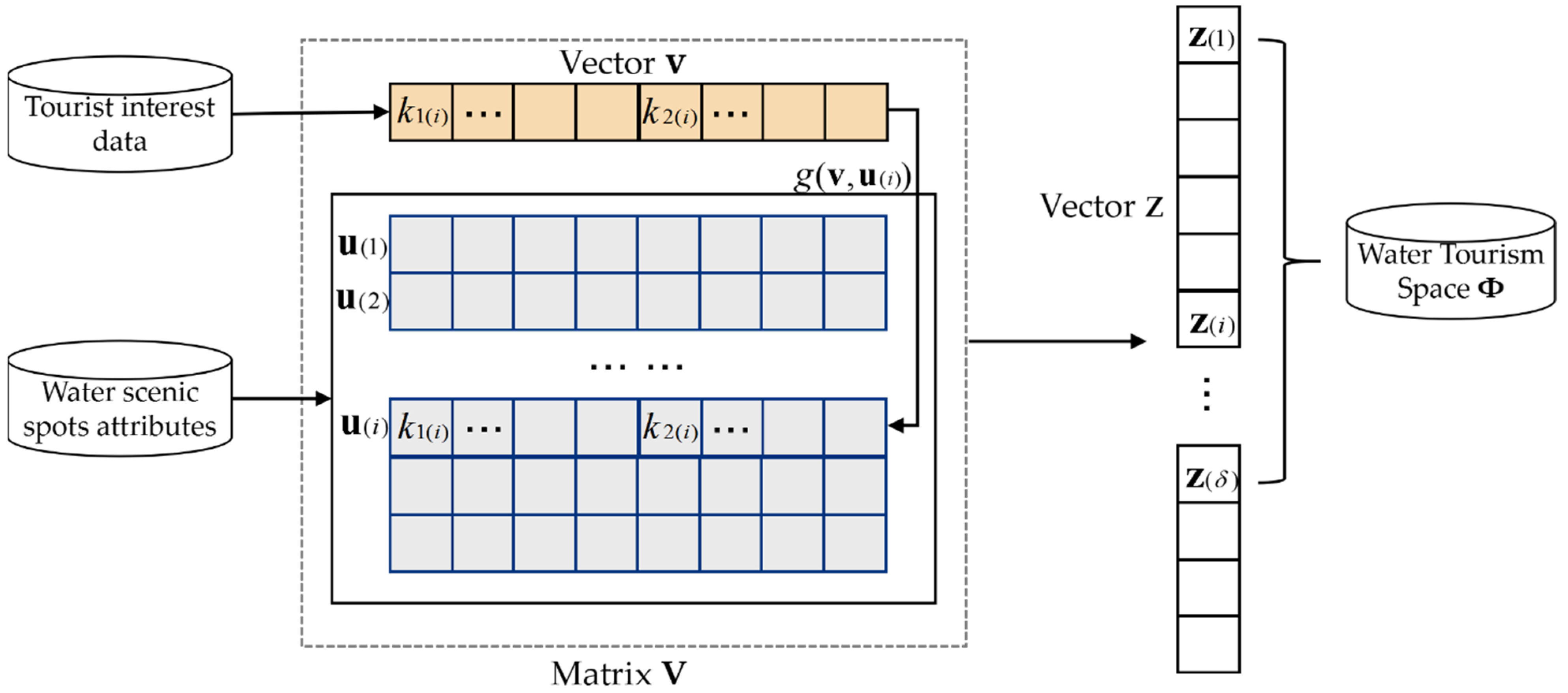
3.1. Water Tourism Space Model Based on Scenic Spot Mining

The precondition to set up the water tourism space and the optimal model on ECER to mine the best matched scenic spots. Thus, it is critical to obtain data on tourists’ interests relating to scenic water spots. The smart machine method provides interest labels for tourists to choose, which rely on scenic water spots’ classifications and attributes. When tourists choose certain labels, the smart machine will recommend a certain number of scenic spots that best match the interest labels. Tourists could confirm a desired traveling sequence according to their schedule [33,34]. Definitions 11–14 are introduced as follows.

Definition 11.

Tourist interest vector $v$. According to the scenic water spot attribute matrix$K$, tourists choose interest labels, and then the labels are quantified and stored into the vector$v$; this vector is defined as the tourist interest vector$v$. It represents a group of interest data. The constraints of vector$v$are as follows:

(1) 

Its dimension is$1\times (m+n)$, in which the$m$represents the$m$number of classifications and$n$represents$n$number of attributes, $n>1$.

(2) 

The former$m$number of elements store the classification labels. The latter number of elements store attribute labels.

(3) 

This ultimately becomes the fully ranked state, namely $rank(v_{(i)})=m+n$.

(4) 

The element is noted as$v(i)$,$0<i\le m+n$, $m,n\in N$.

(5) 

As to the former$m$number of elements, there is at least one value of 1; other elements have values of 0.

Tourists choose specific classifications and attributes from the vector.

Definition 12.

Tourist interest matching matrix$V$. As to the$n*$number of scenic spots$S_{(i)}$in$S_{(0)}$, their attribute matrix$K$could be vectors$u_{(i)}$with the same dimension and rank as$v$. Set the vector$v$as the first row of matrix, and set vectors$u_{(i)}$of the$n*$number of scenic spots$S_{(i)}$as other rows of the matrix; the formed matrix is defined as the tourist interest matching matrix, noted as$V$. According to the definition, vector$u_{(i)}$and matrix$V$meet the following conditions:

(1) 

Its dimension is $1\times (m+n)$, in which the $m$ represents the $m$ number of classifications and $n$ represents $n$ number of attributes, $n>1$.

(2) 

The former $m$ number of elements store the non-zero elements of the first row in matrix $K$. The latter $n$ number of elements store the non-zero elements from the second row in the No. $n+1$ row in matrix $K$.

(3) 

It must be fully ranked, namely $rank(u_{(i)})=m+n$. Each $u_{(i)}$ represents the unique label set for each scenic spot. The element of $u_{(i)}$ is noted as $u_{(i,j)}$, $0<i\le n*$, $0<j\le m+n$, $m,n\in N$.

(4) 

Matrix $V$ has $n*+1$ rows and $m+n$ columns, and they are both fully ranked, namely ${rank(u_{(i)})}_{ro}=n*+1$, ${rank(u_{(i)})}_{co}=m+n$.

(5) 

Two arbitrary rows are nonlinearly correlated, and two arbitrary columns are also nonlinearly correlated.

(6) 

As to the former $m$ number of elements, there is at least on value of 1; the other elements are values of 0.

According to Definitions 11 and 12, each row’s elements of matrix $V$ are stored according to the attribute labels and geographic locations. The first row stores the interest data and positional relations. Other rows are the same data for each scenic spot. The same column relates to one attribute’s data.

Definition 13.

Interest matching objective function$g(v,u_{(i)})$. The matching function between the vector$v$and the vector$u_{(i)}$is defined as the interest matching objective function, noted as$g(v,u_{(i)})$. It determines the correlation between tourists’ needs and scenic spot functions. The function$g(v,u_{(i)})$is set up asEquation (7), in which$k_{1(i)v}$is the selected classification factor by tourists,$k_{1(i)u}$is the scenic water spot classification factor,$\mathsf{\Delta }{k}_{2(i,j)v}$is the selected attribute factor by tourists,$\mathsf{\Delta }{k}_{2(i,j)u}$is the scenic water spot attribute factor, and${\zeta }_{2(i)}$is the normalization parameter.

$$g(v,u_{(i)})={\Vert v-u_{(i)}\Vert }_2={({\displaystyle {\sum }_{i=1}^m{(k_{1(i)v}-k_{1(i)u})}^2}+{\displaystyle {\sum }_{i=1}^n{({\zeta }_{2(i)}\mathsf{\Delta }{k}_{2(i,j)v}-{\zeta }_{2(i)}{k}_{2(i,j)u})}^2})}^{1/2}$$

(7)

Definition 14.

Objective function tab vector$z$. Define the$1\times n*$dimension vector$z$as the objective function tab vector. It is used to dynamically store the function values$g(v,u_{(i)})$. It meets the following conditions. The final elements of vector$z$for the function values$g(v,u_{(i)})$represent the correlations between$S_{(i)}~u_{(i)}$and $v$.

(1) 

The element $z_{(i)}$ relates to the value $g(v,u_{(i)})$.

(2) 

The initial state is a zero matrix, and the final state is fully ranked $rank(z)=n*$.

(3) 

The transition state is a dynamic state of $g(v,u_{(i)})$ value sequencing.

According to the above definitions, the water tourism space model based on scenic spot mining is set up to confirm the best matched scenic water spots for tourists and finally forms the tourism space of the downtown area.

Step 1: Encode each row’s elements of matrix $V$. The first row is the interest vector $v$, and the other rows are vectors $u_{(i)}$. The same column relates to the same attribute. The basic encoding method is as follows:

(1)

The former $m$ number of elements in the first row are the classification factors $k_{1(1)}$, $k_{1(2)}$, …, $k_{1(m)}$, relating to the $m$ number of classifications of the vector $k_1$. The latter $n$ number of elements in the first row are the selected attribute factors, relating to the $n$ number of attributes $k_{2(1)}$, $k_{2(2)}$, …, $k_{2(n)}$. The latter rows have the same storage mode as the first row.

(2)

The second row to the last, No. $n*+1$ row, is encoded as $u_{(1)}$, $u_{(2)}$, …, $u_{(n*)}$. The function values $g(v,u_{(i)})$ do not match the code $u_{(i)}$.

(3)

The later $n*$ number of rows do not match the element $z_{(i)}$ of vector $z$.

Step 2: Calculate and store the No. 1 and No. 2 element of vector $z$.

Sub-step 1: Calculate the objective function value $g(v,u_{(1)})$ between the first row $v$ and row $u_{(1)}$, and store the value into the element $z_{(1)}$.

Sub-step 2: Calculate the objective function value $g(v,u_{(2)})$ between the first row $v$ and row $u_{(2)}$, and store the value in the element $z_{(2)}$.

Sub-step 3: Compare the value $g(v,u_{(1)})$ and $g(v,u_{(2)})$.

(1)

If $g(v,u_{(1)})\le g(v,u_{(2)})$, keep the element values unchanged.

(2)

If $g(v,u_{(2)})<g(v,u_{(1)})$, delete the values in $z_{(1)}$ and $z_{(2)}$. Store $g(v,u_{(2)})$ in $z_{(1)}$ and store $g(v,u_{(1)})$ in $z_{(2)}$.

Sub-step 4: Calculate the objective function value $g(v,u_{(3)})$ between the first row $v$ and row $u_{(3)}$, and store the value in the element $z_{(3)}$ and then make a comparison.

(1)

If $g(v,u_{(1)})\le g(v,u_{(2)})$:

①

If $g(v,u_{(3)})<g(v,u_{(1)})\le g(v,u_{(2)})$, delete the storage values of $z_{(1)}$ and $z_{(2)}$, store $g(v,u_{(3)})$ in $z_{(1)}$, store $g(v,u_{(1)})$ in $z_{(2)}$ and store $g(v,u_{(2)})$ in $z_{(3)}$;

②

If $g(v,u_{(1)})<g(v,u_{(3)})\le g(v,u_{(2)})$, keep the $z_{(1)}$ storage value, delete $z_{(2)}$ storage value, store $g(v,u_{(3)})$ in $z_{(2)}$ and store $g(v,u_{(2)})$ in $z_{(3)}$;

③

If $g(v,u_{(1)})\le g(v,u_{(2)})<g(v,u_{(3)})$, keep the $z_{(1)}$ and $z_{(2)}$ storage value, and store $g(v,u_{(3)})$ in $z_{(3)}$.

(2)

If $g(v,u_{(2)})<g(v,u_{(1)})$:

①

If $g(v,u_{(3)})<g(v,u_{(2)})<g(v,u_{(1)})$, delete the storage values of $z_{(1)}$ and $z_{(2)}$, store $g(v,u_{(3)})$ in $z_{(1)}$, store $g(v,u_{(2)})$ in $z_{(2)}$ and store $g(v,u_{(1)})$ in $z_{(3)}$;

②

If $g(v,u_{(2)})<g(v,u_{(3)})<g(v,u_{(1)})$, keep $z_{(1)}$ storage value, delete $z_{(2)}$ storage value, store $g(v,u_{(3)})$ in $z_{(2)}$ and store $g(v,u_{(1)})$ in $z_{(3)}$;

③

If $g(v,u_{(2)})<g(v,u_{(1)})<g(v,u_{(3)})$, keep $z_{(1)}$ and $z_{(2)}$ storage values, and store $g(v,u_{(3)})$ in $z_{(3)}$.

Sub-step 5: Repeat Sub-steps 1–4. Calculate the objective function value $g(v,u_{(i)})$ between the first row $v$ and row $u_{(i)}$, traverse the range $i~[4,n*]\subset N$. Make a comparison between the current $g(v,u_{(i)})$ and $g(v,u_{(1)})$, $g(v,u_{(2)})$, …, $g(v,u_{(i-1)})$. The smaller values are always stored in the smaller footnote elements $z_{(i)}$, in which the vector $u_{(i)}$ with smaller function value $g(v,u_{(i)})$ has a closer correlation to the interest vector $v$.

Sub-step 6: Tourists input the quantity of the scenic spots to be visited in a tour day. The criterion to make the selection is set as follows:

(1)

Tourists have no requirements on cluster $S_{(i)}$. Input the scenic spot quantity $\delta$, the smart machine searches the former $\delta$ number of elements $z_{(i)}$, and take the related $g(v,u_{(i)})$, vector $u_{(i)}$ and scenic spot $S_{(i)}$.

(2)

Tourists have requirements on cluster $S_{(i)}$. Tourists choose $c$ number of $S_{(i)}*$ and the quantity ${\delta }_{(i)}$ of scenic spots to be visited in each cluster $S_{(i)}$. Set counter for each cluster as ${\lambda }_{(i)}$, the initial value is ${\lambda }_{(i)}=0$, $0<c\le k$, $c,k\in N$, $k$ is the total number of cluster $S_{(i)}$.

①

Search the No. 1 element $z_{(1)}$ of the vector $z$. Confirm the related $g(v,u_{(i)})$, vector $u_{(i)}$ and scenic spot $S_{(i)}{z}_{(1)}$:

(i)

If $S_{(i)}{z}_{(1)}\in \forall S_{(i)}*$, keep $S_{(i)}{z}_{(1)}$, $\lambda =\lambda +1$, turn to step ③.

(ii)

If $S_{(i)}{z}_{(1)}\notin \forall S_{(i)}*$, delete.

②

Search the No. $i$ element $z_{(i)}$ of the vector $z$,$i~[2,n*]\subset N$. Confirm the related $g(v,u_{(i)})$, vector $u_{(i)}$ and scenic spot $S_{(i)}{z}_{(1)}$:

(i)

If $S_{(i)}{z}_{(1)}\in \forall S_{(i)}*$, keep $S_{(i)}{z}_{(1)}$, $\lambda =\lambda +1$, turn to step ③.

(ii)

If $S_{(i)}{z}_{(1)}\notin \forall S_{(i)}*$, delete.

③

Judge the counter ${\lambda }_{(i)}$:

(i)

If $\exists \forall {\lambda }_{(i)}<{\delta }_{(i)}$, go back to step ② and continue searching the scenic spots for this cluster $S_{(i)}*$.

(ii)

If $\forall {\lambda }_{(i)}={\delta }_{(i)}$ and ${\displaystyle {\sum }_{i=0}^c}{\delta }_{(i)}=\delta$, the algorithm ends. Output scenic spots $S_{(i)}*$ of each cluster $S_{(i)}*$.

According to the clusters and scenic spots confirmed by the tourists’ needs and the proposed algorithm, make visualization maps for the clusters, the selected scenic spots and the tourism space $\mathsf{\Phi }$. Figure 1 shows the process to form the tourism space $\mathsf{\Phi }$.

3.2. Optimal ECER Tour Route Algorithm Based on the Water Tourism Space

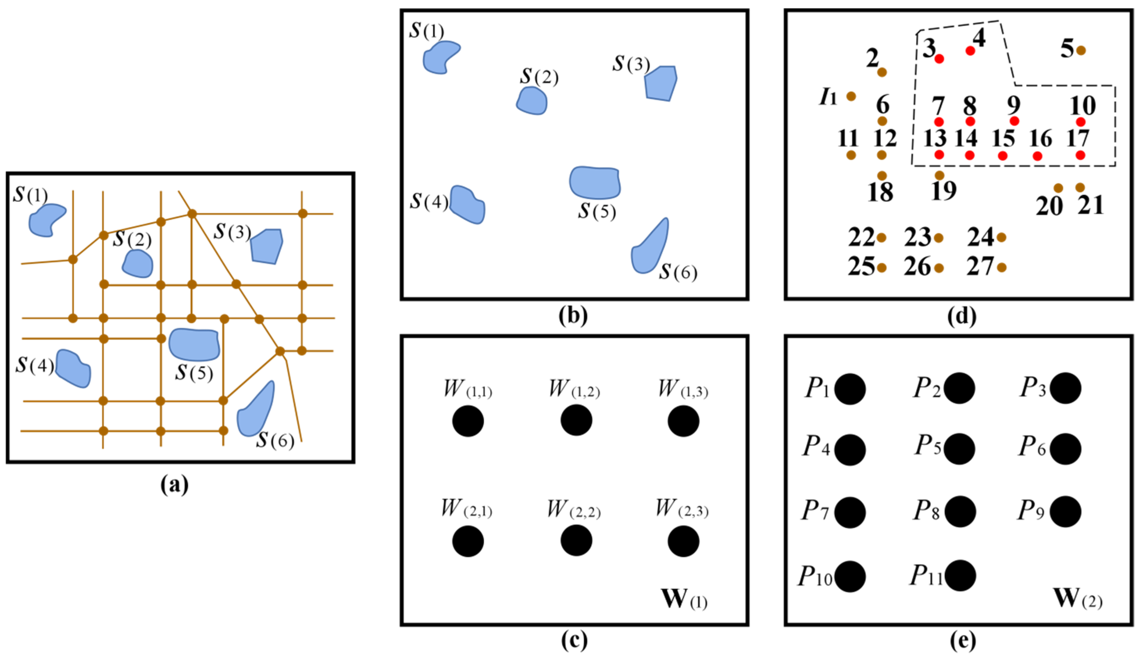
When tourists travel in the water tourism space, they should travel along the routes with the lowest costs. Meanwhile, considering the protection of the urban ecosystems and low-carbon requirements, when tourists choose motor vehicles, it is necessary for them to reduce the consumption of energy and exhaust emissions, thus decreasing the damage to the city water resources. Usually, tourists tend to take motor vehicles to save travel time, as they are efficient and fast. However, this also brings exhaust emissions. Thus, in the constraint of the total time, decreasing the whole route distance and reducing the ferrying time could help increase the scenic spot visiting time and reduce exhaust emissions [35,36,37]. The optimal ECER tour route algorithm based on the water tourism space is set up according to Definitions 15–20.

Definition 15.

First order matrix model$W_{(1)}$of the water tourism space. The scenic water spots distributed in the space$\mathsf{\Phi }$are converted to the matrix lattice according to the quantity$\delta$of scenic spots to be visited. The matrix lattice that is used to store the scenic water spots is defined as the first order matrix model of the water tourism space, noted as$W_{(1)}$. The constraints for$W_{(1)}$are as follows:

(1) 

Scenic water spots$S_{(i)}$are abstracted as the space lattice with longitude and latitude, according to their spatial distribution.

(2) 

Its dimension is$(\lfloor \sqrt{\delta }\rfloor +1)\times (\lfloor \sqrt{\delta }\rfloor +1)$, the row and column’s full ranks are both $rank(W_{(1)})=\lfloor \sqrt{\delta }\rfloor +1$.

(3) 

Starting from the first element in the first row and ending at the last element of the No.$\lfloor \sqrt{\delta }\rfloor +1$row, the scenic spots$S_{(i)}$are stored in spatial sequence.

(4) 

Empty elements are set as value 0.

Definition 16.

Motor vehicle path set $R$and intersection set$P$. Scenic spots are connected by city roads. According to the definition of city geography, city roads can be divided into several grades. In a city, the roads on which private cars, taxis, and online ride-hailing cars could are classified as motor vehicle accessible roads. Store the accessible roads in a set; this set is defined as the motor vehicle path set$R$. Store the intersections of all the accessible roads in set$P$. The arbitrary intersection$P$of$R_{(i)}$and$R_{(j)}$is an accessible intersection. The effective intersections$P$are selected to set up the algorithm; these are those which the tourists will be most likely to pass.

Definition 17.

Second order matrix model $W_{(2)}$ of the water tourism space. Take arbitrary two elements $W_{(i_1,j_1)}$ and $W_{(i_2,j_2)}$ in $W_{(1)}$, and extract a certain number of effective intersections $P$ between $W_{(i_1,j_1)}$ and $W_{(i_2,j_2)}$ in $P$. The effective intersection set $P*$ forms the ferry space between two scenic spots. Define the set that contains all the effective intersections in $P*$ as the second order matrix model of the water tourism space, noted as $W_{(2)}$. Set the number of the effective intersections in $W_{(2)}$ as $\varphi$. The constraints for the $W_{(2)}$ are as follows:

(1) 

Effective intersections$P$are abstracted as the space lattice with longitude and latitude, according to their spatial distribution.

(2) 

Its dimension is$(\lfloor \sqrt{\varphi }\rfloor +1)\times (\lfloor \sqrt{\varphi }\rfloor +1)$, the row and column’s full ranks are both $rank(W_{(2)})=\lfloor \sqrt{\varphi }\rfloor +1$.

(3) 

Starting from the first element in the first row and ending at the last element of the No.$\lfloor \sqrt{\varphi }\rfloor +1$row, the effective intersections$P$are stored in spatial sequence.

(4) 

Empty elements are set as value 0.

Figure 2 is the process of abstracting the tourism space $\mathsf{\Phi }$ into the model $W_{(1)}$ and $W_{(2)}$. The model is the precondition to set up the optimal ECER tour route algorithm based on the water tourism space. Figure 2a shows the distribution of the scenic water spots, connecting roads and road intersections in the water tourism space $\mathsf{\Phi }$. Figure 2b shows the scenic water spots’ distribution. Figure 2c shows the built $W_{(1)}$ model based on Figure 2b. Figure 2d shows the road intersection set in the space $\mathsf{\Phi }$ and the effective intersection set between the scenic spots $S_{(2)}$ and $S_{(3)}$, noted by the red points in the dashed frame. Figure 2e shows the built $W_{(2)}$ model based on Figure 2d.

Definition 18.

Basic ECER unit$E_n$. When a motor vehicle takes tourists from$W_{(i_1,j_1)}$to$W_{(i_2,j_2)}$, the average exhaust emission volume of the motor vehicle per kilometer is defined as the basic ECER unit, noted as$E_n$. In the algorithm, it is measured by the gas weight, unit: kg.

When the car model is confirmed, it could be considered that the $E_n$ is a constant value. When the constant value $E_n$ is confirmed, the total exhaust emission of the motor vehicle is directly proportional to the traveling distance in a tour route. Thus, setting up an optimal route model to reduce the total ferrying distance between scenic spots could effectively decrease the exhaust emission volume.

Definition 19.

Scenic spot path structure tree $T_{(o)}$. Based on the$W_{(2)}$between$W_{(i_1,j_1)}$and$W_{(i_2,j_2)}$, the travel path connecting$W_{(i_1,j_1)}$and$W_{(i_2,j_2)}$through the effective intersection set$P*$is created. The structure tree that is formed by$W_{(i_1,j_1)}$,$W_{(i_2,j_2)}$and$P$in set$P*$is defined as scenic spot path structure tree $T_{(o)}$. Tree$T_{(o)}$should meet the following conditions$C_{(T_{(o)})}$:

(1) 

It is a connected graph that does not contain a simple loop.

(2) 

Vertex$W_{(i_1,j_1)}$or$W_{(i_2,j_2)}$is only connected by one edge. Node$P$must have two connecting edges.

(3) 

Any two vertexes$u$and$v$can only have one connecting edge.

(4) 

It is a directed graph from$W_{(i_1,j_1)}$to $W_{(i_2,j_2)}$.

(5) 

The edge weight of the vertexes$u$and$v$is the spatial distance.

When a tree $T_{(o)}$ contains $k$ number of vertexes, it must have $k-1$ number of edges. The total ECER volume $E_{n(o)}*$ of the tree $T_{(o)}$ is modeled as Equation (8).

$$E_{n(o)}*={\displaystyle {\sum }_{x=1}^{k-1}{E}_n\cdot d_{{(u,v)}_{(x)}}}$$

(8)

Definition 20.

Total ECER volume storage vector $E_n*$. When the tree$E_n*$is built and the total ECER volume is calculated, store the volumes$E_{n(o)}*$in a$1\times q$dimension vector; this vector is defined as the total ECER volume storage vector $E_n*$, in which$q$is the maximum quantity of the tree $T_{(o)}$.

According to the definitions, the optimal ECER tour route algorithm based on the water tourism space is set up as follows:

Step 1: Set up the ECER model for $W_{(2)}$. The model $W_{(2)}$ is the substructure of the tourism space $\mathsf{\Phi }$. The optimal tour route algorithm in $W_{(2)}$ is set up first.

Sub-step 1: Build the tree $T_{(1)}$ and calculate the ECER volume $E_{n\left(1\right)}*$. Figure 3 shows the process to build the tree $T_{(1)}$.

(1)

The initial state is shown in Figure 3a. The space lattice is $W_{(2)}$, containing $W_{(i_1,j_1)}$ and $W_{(i_2,j_2)}$. The starting point is $W_{(i_1,j_1)}$ while the ending point is $W_{(i_2,j_2)}$. Absorb $W_{(i_1,j_1)}$ into $T_{(1)}$.

(2)

Judge the edge $d_{(W_{(i_1,j_1)},P_x)}$, in which the $x$ values are 1, 2, 5, 8 and 9. Confirm the smallest edge weight $d_{(W_{(i_1,j_1)},P_5)}$. Search the $W_{(i_1,j_1)}$ and edge $e_{(1)}$ of $P_5$, shown in Figure 3b. Make a judgement: ① If $e_{(1)}$ and $P_5$ meet $C_{(T_{(o)})}$, absorb $e_{(1)}$ and $P_5$ into $T_{(1)}$; ② If $e_{(1)}$ and $P_5$ do not meet $C_{(T_{(o)})}$, delete. Search the other points $P_i$.

(3)

Continue searching the smallest edge weight as in Steps (1)–(2). Find the $P_9$, and form the edge $e_{(2)}$, as shown in Figure 3c. Judge that it meets $C_{(T_{(o)})}$, and absorb $e_{(2)}$ and $P_9$ into $T_{(1)}$.

(4)

Find the $P_6$, and form the edge $e_{(3)}$, as shown in Figure 3d. Judge that it meets $C_{(T_{(o)})}$, and absorb $e_{(3)}$ and $P_6$ into $T_{(1)}$.

(5)

Continue searching; when $P_5$ is found, it forms a loop; then delete $P_5$. Find $P_7$ and form the edge $e_{(4)}$, shown as Figure 3e. Judge that it meets $C_{(T_{(o)})}$, and absorb $e_{(4)}$ and $P_7$ into $T_{(1)}$.

(6)

Find the ending point $W_{(i_2,j_2)}$ and absorb it into $T_{(1)}$, as shown in Figure 3f.

(7)

Calculate the ECER volume $E_{n\left(1\right)}*$ of $T_{(1)}$, and store it into the first element $E_{n(1)}*$ of $E_n*$. Here, the searching process ends.

Sub-step 2: Build the tree $T_{(2)}$ and calculate the ECER volume $E_{n\left(2\right)}*$; store $E_{n\left(2\right)}*$ in the second element $E_{n(2)}*$ of $E_n*$, and compare $E_{n\left(1\right)}*$ with $E_{n\left(2\right)}*$.

(1)

If $E_{n\left(1\right)}*>E_{n\left(2\right)}*$, delete $E_{n\left(1\right)}*$ and $E_{n\left(2\right)}*$, store $E_{n\left(1\right)}*$ in $E_{n(2)}*$, store $E_{n\left(2\right)}*$ in $E_{n(1)}*$;

(2)

If $E_{n\left(1\right)}*<E_{n\left(2\right)}*$, keep $E_{n\left(1\right)}*$ and $E_{n\left(2\right)}*$.

Sub-step 3: Repeat the above sub-steps. Build the tree $T_{(o)}$ and calculate the ECER volume $E_{n\left(o\right)}*$; store $E_{n\left(o\right)}*$ in the element $E_{n(o)}*$ of $E_n*$, and compare $E_{n\left(1\right)}*$ to $E_{n\left(\mathrm{o}\right)}*$. The element $E_{n(o)}*$ should meet the following conditions:

(1)

Vector $E_n*$ is fully ranked, namely $W_{(2)}$ $rank(E_n*)=q$.

(2)

$0<o\le q$, $o\in N$, if $o_i<o_j$, there is always $E_{n(oi)}*<E_{n(oj)}*$.

Sub-step 4: Take the total ECER volume $E_{n\left(oi\right)}*$ of the first element $E_{n(1)}*$ in $E_n*$. Its related tree $T_{(oi)}$ is the optimal path between $W_{(i_1,j_1)}$ and $W_{(i_2,j_2)}$.

Step 2: Set up the ECER model for $W_{(1)}$. The $\delta$ number of scenic spots selected by the smart machine cover different clusters and have specific locations. When tourists travel in the space $\mathsf{\Phi }$, they first choose the favorite sequence on the scenic spots, that is, in the model $W_{(1)}$, the optimal tour route is searched by the model, which finally accumulates the optimal tour route in the whole $W_{(1)}$ with the lowest energy consumption and exhaust emission. When a tourist confirms a type of sequence, the ECER model for $W_{(1)}$ is set up as follows:

Sub-step 1: Build the scenic water spot tour sequence vector $Q$ based on $W_{(1)}$. Build a $1\times (\delta +1)$ dimension vector $Q$ to store the $\delta$ number of scenic spots and the starting point. The constraints for the vector $Q$ are as follows:

(1)

The element is $Q_{(i)}$, and it is fully ranked, namely $rank(Q_{(i)})=\delta$.

(2)

Element $Q_{(1)}$ is used to store the starting point $S_t$. Elements $Q_{(2)}$~$Q_{(\delta +1)}$ are used to store the $\delta$ number of scenic spots in the tour sequence.

(3)

Element $Q_{(i)}$ and $Q_{(i+1)}$ are the two adjacent scenic spots, and the spatial interval is $W_{(2)}$.

(4)

$Q_{(1)}$~$Q_{(\delta +1)}$ as well as their spatial intervals $W_{(2)}$ form a complete tour sequence in the space $\mathsf{\Phi }$.

Sub-step 2: Calculate the total ECER volume $E_{n\left(1\right)}*$ between $Q_{(1)}$ and $Q_{(2)}$, and store the value.

Sub-step 3: Calculate the total ECER volume $E_{n\left(i\right)}*$ between $Q_{(i)}$ and $Q_{(i+1)}$, $1<i\le \delta$, $i\in N$, and store the value.

Sub-step 4: Calculate the total ECER volume $E_{n(to)}$ of the complete tour sequence, as shown in Formula (9).

$$E_{n(to)}={\displaystyle {\sum }_{i=1}^{\delta }{E}_{n(i)}*}$$

(9)

4. Experiment and Result Analysis

In order to verify the feasibility and advantages of the proposed algorithm, an experiment was designed. We chose the tourism city Chengdu and its 24 urban scenic water spots as the research range and objects. They cover multiple tour functions, classifications and attributes, which can satisfy different tourists. The basic principle of the experiment is as follows: Confirm the scenic water spots and quantify their classifications and attributes. Use the proposed improved DIANA algorithm to form scenic spot clusters. Confirm the best matched scenic spots according to tourists’ needs, and then search the optimal ECER tour routes. Finally, the tourists’ frequently used electronic maps are set as the control group to allow comparison and verify that the proposed algorithm is feasible and has advantages. The raw data for the experiment are obtained from the basic geographic information data and traffic information data of Chengdu city. The names and attributes of the scenic water spots are obtained from the official website of Baidu Encyclopedia and the Chengdu City Platform for Common Geospatial Information Services. The traffic information data is used to calculate the results are obtained from the Chengdu City Platform for Common Geospatial Information Services and Chengdu City Public Data Open Platform, as well as Chengdu City’s electronic map.

4.1. The Acquisition of the Scenic Water Spots and Calculation Results

The selected typical scenic water spots in the Chengdu downtown area are: $S_{(1)}$: Jincheng Lake Park; $S_{(2)}$: Qinglonghu Reservoir; $S_{(3)}$: Bailuwan Wetland Park; $S_{(4)}$: Zhonghe Wetland Park; $S_{(5)}$: East Lake; $S_{(6)}$: South Lake; $S_{(7)}$: North Lake; $S_{(8)}$: Huanhua Brook and Dufu Cottage; $S_{(9)}$: Chengdu Happy Valley; $S_{(10)}$: Shengxian Lake; $S_{(11)}$: Wangjianglou Park; $S_{(12)}$: Shahe City Park; $S_{(13)}$: Xinglong Lake; $S_{(14)}$: People’s Park; $S_{(15)}$: Xinhua Park; $S_{(16)}$: Jiaozi Park; $S_{(17)}$: Xinzhendi Golf Club; $S_{(18)}$: Boya Sports Club; $S_{(19)}$: International Intangible Cultural Heritage Expo Park; $S_{(20)}$: Lianghe City Forest Park; $S_{(21)}$: Shahe Park; $S_{(22)}$: Sansheng Flower Town; $S_{(23)}$: Funanhe Flowing Water Park; $S_{(24)}$: Shibashan Cross-Country Park.

Table 1. Scenic water spot normalized classifications and attributes.

	$k_{1(1)}$	$k_{1(2)}$	$k_{1(3)}$	$k_{1(4)}$	$k_{2(1)}$	$k_{2(2)}$	$k_{2(3)}$	$k_{2(4)}$
$S_{(1)}$	1.00	0.00	0.00	1.00	0.36	0.00	0.20	0.14
$S_{(2)}$	1.00	0.00	0.00	1.00	0.28	0.00	0.20	0.13
$S_{(3)}$	1.00	0.00	0.00	1.00	0.44	0.00	0.20	0.16
$S_{(4)}$	1.00	0.00	0.00	1.00	0.25	0.00	0.15	0.15
$S_{(5)}$	1.00	0.00	0.00	1.00	0.45	0.00	0.15	0.09
$S_{(6)}$	1.00	0.00	0.00	1.00	0.31	0.00	0.15	0.22
$S_{(7)}$	1.00	0.00	0.00	1.00	0.28	0.00	0.15	0.08
$S_{(8)}$	1.00	0.00	1.00	0.00	0.68	0.50	0.20	0.06
$S_{(9)}$	1.00	1.00	0.00	1.00	0.72	2.30	0.20	0.05
$S_{(10)}$	1.00	0.00	0.00	1.00	0.45	0.00	0.15	0.02
$S_{(11)}$	1.00	0.00	1.00	0.00	0.62	0.00	0.15	0.08
$S_{(12)}$	1.00	0.00	0.00	1.00	0.56	0.00	0.10	0.06
$S_{(13)}$	1.00	0.00	0.00	1.00	0.38	0.00	0.15	0.33
$S_{(14)}$	1.00	1.00	1.00	1.00	0.72	0.00	0.20	0.05
$S_{(15)}$	1.00	1.00	1.00	1.00	0.70	0.00	0.20	0.06
$S_{(16)}$	1.00	0.00	0.00	1.00	0.55	0.00	0.15	0.13
$S_{(17)}$	1.00	0.00	0.00	1.00	0.30	0.00	0.20	0.10
$S_{(18)}$	1.00	0.00	0.00	1.00	0.30	0.00	0.20	0.14
$S_{(19)}$	1.00	0.00	1.00	0.00	0.25	0.35	0.20	0.15
$S_{(20)}$	1.00	0.00	0.00	1.00	0.42	0.00	0.15	0.11
$S_{(21)}$	1.00	0.00	0.00	0.00	0.46	0.00	0.15	0.03
$S_{(22)}$	1.00	0.00	0.00	1.00	0.52	0.00	0.20	0.15
$S_{(23)}$	1.00	0.00	0.00	1.00	0.45	0.00	0.15	0.04
$S_{(24)}$	1.00	1.00	0.00	1.00	0.28	0.00	0.15	0.14

shows each scenic water spot’s normalized classifications and attributes, in which $k_{2(i)}$ relates to the classification and $k_{2(i)}$ relates to attributes: $k_{1(1)}$: recreation and sightseeing; $k_{1(2)}$: boating experience; $k_{1(3)}$: culture and custom; $k_{1(4)}$: water sports; $k_{2(1)}$: the popularity degree; $k_{2(2)}$: the minimum cost; $k_{2(3)}$: the traveling time; $k_{2(4)}$: the spatial distance. The starting point of the tourist is Chengdu railway station, which is used to calculate the spatial distance. The spatial distance is calculated from the longitude and latitude. Figure 4 shows the scenic water spots map of Chengdu city; Figure 4a shows the scenic water spot geographic spatial distribution, and Figure 4b shows the initial cluster $S_{(0)}$ formed by the extracted scenic water spots.

4.2. The Results of Scenic Water Spot Clustering and Cluster Visualization

Calculate each scenic spot’s average dissimilarity using the data in Table 1; the results are shown in

Table 2. The output result of each scenic spot’s average dissimilarity (four decimal places).

$S_{(i)}$	$i=1$	$i=2$	$i=3$	$i=4$	$i=5$	$i=6$
$t(S_{(i)},S_{(i)})$	0.6015	0.5970	0.5812	0.6138	0.5773	0.6070
$S_{(i)}$	$i=7$	$i=8$	$i=9$	$i=10$	$i=11$	$i=12$
$t(S_{(i)},S_{(i)})$	0.6029	1.4168	2.4434	0.5972	1.3556	0.6306
$S_{(i)}$	$i=13$	$i=14$	$i=15$	$i=16$	$i=17$	$i=18$
$t(S_{(i)},S_{(i)})$	0.6529	1.3824	1.3784	0.6124	0.5912	0.5895
$S_{(i)}$	$i=19$	$i=20$	$i=21$	$i=22$	$i=23$	$i=24$
$t(S_{(i)},S_{(i)})$	1.3778	0.5723	1.1301	0.6029	0.5892	1.1488

. When the cluster quantities are set as $k=2$, $k=3$, $k=4$, $k=5$, the clusters and related scenic spots are formed, as shown in

Table 3. Each cluster’s output result under different cluster quantity conditions.

$\mathit{k}$	Center Point ${\mathit{S}}_{(\mathit{i})}*$	Cluster ${\mathit{S}}_{(\mathit{i})}$ Output Result
$k=2$	$S_{(20)}$, $S_{(5)}$	$S_{(1)}$: $S_{(20)}$, $S_{(1)}$, $S_{(2)}$, $S_{(3)}$, $S_{(4)}$, $S_{(6)}$, $S_{(7)}$, $S_{(13)}$, $S_{(17)}$, $S_{(18)}$, $S_{(19)}$, $S_{(24)}$
		$S_{(2)}$: $S_{(5)}$, $S_{(8)}$, $S_{(9)}$, $S_{(10)}$, $S_{(11)}$, $S_{(12)}$, $S_{(14)}$, $S_{(15)}$, $S_{(16)}$, $S_{(21)}$, $S_{(22)}$, $S_{(23)}$
$k=3$	$S_{(20)}$, $S_{(5)}$, $S_{(3)}$	$S_{(1)}$: $S_{(20)}$, $S_{(2)}$, $S_{(4)}$, $S_{(7)}$, $S_{(17)}$, $S_{(18)}$, $S_{(19)}$, $S_{(24)}$
		$S_{(2)}$: $S_{(5)}$, $S_{(8)}$, $S_{(9)}$, $S_{(10)}$, $S_{(11)}$, $S_{(12)}$, $S_{(14)}$, $S_{(15)}$, $S_{(16)}$, $S_{(21)}$, $S_{(23)}$
		$S_{(3)}$: $S_{(3)}$, $S_{(1)}$, $S_{(6)}$, $S_{(13)}$, $S_{(22)}$
$k=4$	$S_{(20)}$, $S_{(5)}$, $S_{(3)}$, $S_{(23)}$	$S_{(1)}$: $S_{(20)}$, $S_{(2)}$, $S_{(4)}$, $S_{(7)}$, $S_{(17)}$, $S_{(18)}$, $S_{(19)}$, $S_{(24)}$
		$S_{(2)}$: $S_{(5)}$, $S_{(11)}$, $S_{(16)}$
		$S_{(3)}$: $S_{(3)}$, $S_{(1)}$, $S_{(6)}$, $S_{(13)}$, $S_{(22)}$
		$S_{(4)}$: $S_{(23)}$, $S_{(8)}$, $S_{(9)}$, $S_{(10)}$, $S_{(12)}$, $S_{(14)}$, $S_{(15)}$, $S_{(21)}$
$k=5$	$S_{(20)}$, $S_{(5)}$, $S_{(3)}$, $S_{(23)}$, $S_{(18)}$	$S_{(1)}$: $S_{(20)}$
		$S_{(2)}$: $S_{(5)}$, $S_{(11)}$, $S_{(16)}$
		$S_{(3)}$: $S_{(3)}$, $S_{(13)}$, $S_{(22)}$
		$S_{(4)}$: $S_{(23)}$, $S_{(8)}$, $S_{(9)}$, $S_{(10)}$, $S_{(12)}$, $S_{(14)}$, $S_{(15)}$, $S_{(21)}$
		$S_{(5)}$: $S_{(18)}$, $S_{(1)}$, $S_{(2)}$, $S_{(4)}$, $S_{(6)}$, $S_{(7)}$, $S_{(17)}$, $S_{(19)}$, $S_{(24)}$

. Figure 5 shows the visualization results of the clusters under different cluster quantity conditions; the small blue ranges are the miniature scenic spots. After connecting the two ranges in the sequence of clustering, the topology edges, structure trees and cluster topology ranges are obtained.

4.3. The Results of the Optimal Scenic Spots and Tour Routes

In a tour day, the tourist confirms the interest labels according to the output clusters and scenic spot attributes. The smart machine calculates and generates the interest vector $v$ and interest matching matrix $V$ and calculates the objective function values $g(v,u_{(i)})$.

Table 4. The output results of the objective function values $g(v,u_{(i)})$.

	$S_{(1)}$	$S_{(2)}$	$S_{(3)}$	$S_{(4)}$	$S_{(5)}$	$S_{(6)}$	$S_{(7)}$	$S_{(8)}$
$g(v,u_{(i)})$	0.2823	0.3490	0.2317	0.3808	0.1749	0.3640	0.3298	1.5042
	$S_{(9)}$	$S_{(10)}$	$S_{(11)}$	$S_{(12)}$	$S_{(13)}$	$S_{(14)}$	$S_{(15)}$	$S_{(16)}$
$g(v,u_{(i)})$	2.5119	0.1513	1.4166	0.0877	0.3966	1.4211	1.4199	0.1393
	$S_{(17)}$	$S_{(18)}$	$S_{(19)}$	$S_{(20)}$	$S_{(21)}$	$S_{(22)}$	$S_{(23)}$	$S_{(24)}$
$g(v,u_{(i)})$	0.3202	0.3348	1.5067	0.2110	1.0102	0.1772	0.1552	1.0592

shows the output results of the objective function values $g(v,u_{(i)})$. Based on the Table 4 data, the smart machine recommends each cluster’s optimal scenic spots for the tourist. The tourist confirms five scenic spots to be visited according to the calculation results and then confirms the tour sequence $Q$ according to their interests.

In the experiment, the interest labels confirmed by the tourist are (1) Enjoy the scenery and take photos; (2) do not enjoy boating or splashing; (3) there are no requirements for appreciating water scenery cultures or customs; (4) desire to wander around and do leisure sports. In addition, for one single scenic spot: (5) the popularity degree is set at 0.60; (6) the lowest cost is set at 0; (7) visiting time in a scenic spot is set at 1.50; (8) the maximum distance to the starting point is 20 km, and the nearer the better. Based on the interest labels, the interest vector is output $v$ = {1.00, 0.00, 0.00, 1.00, 0.60, 0.00, 0.15, 0.00}.

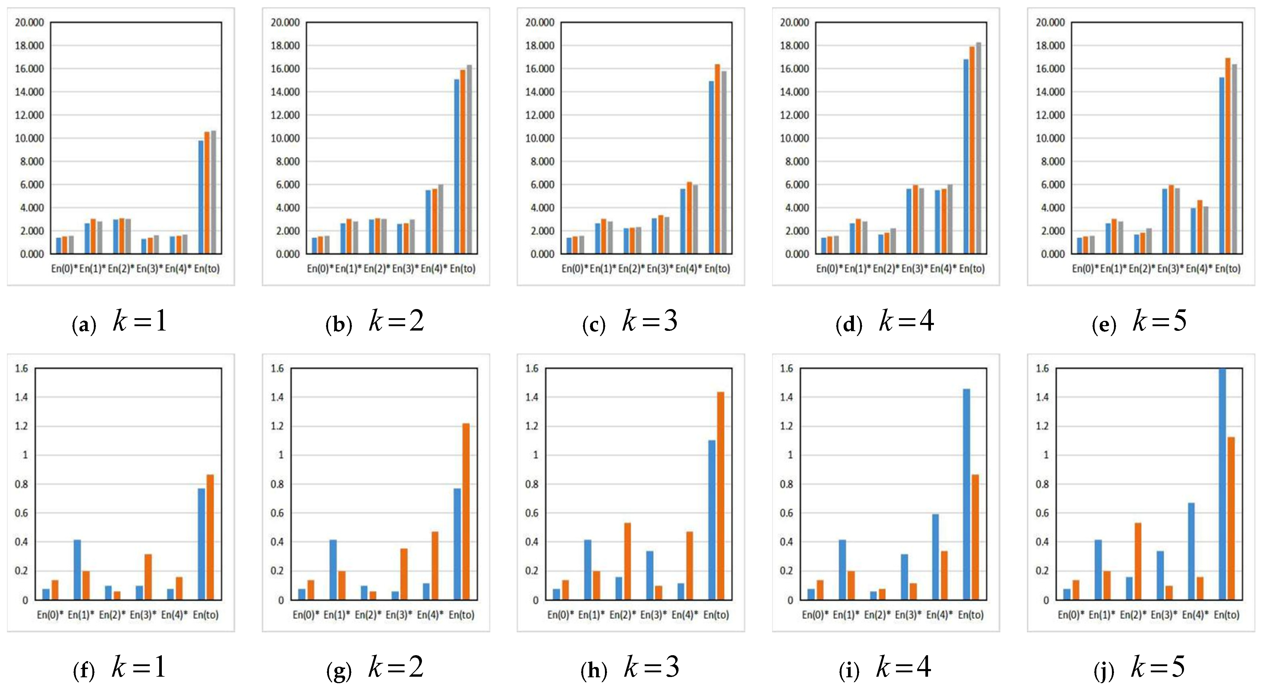
4.4. Comparison of Results

Based on the

Table 5. The scenic spot tour sequence vector $Q$ under the cluster quantity conditions.

	$Q_{\mathbf{(}\mathbf{1}\mathbf{)}}$	$Q_{\mathbf{(}\mathbf{2}\mathbf{)}}$	$Q_{\mathbf{(}\mathbf{3}\mathbf{)}}$	$Q_{\mathbf{(}\mathbf{4}\mathbf{)}}$	$Q_{\mathbf{(}\mathbf{5}\mathbf{)}}$
$k=1$	$S_{(12)}$	$S_{(16)}$	$S_{(10)}$	$S_{(23)}$	$S_{(5)}$
$k=2$	$S_{(12)}$	$S_{(16)}$	$S_{(10)}$	$S_{(20)}$	$S_{(3)}$
$k=3$	$S_{(12)}$	$S_{(16)}$	$S_{(22)}$	$S_{(20)}$	$S_{(3)}$
$k=4$	$S_{(12)}$	$S_{(16)}$	$S_{(23)}$	$S_{(22)}$	$S_{(20)}$
$k=5$	$S_{(12)}$	$S_{(16)}$	$S_{(22)}$	$S_{(20)}$	$S_{(1)}$

data and the tour sequences, the models $W_{(1)}$ and $W_{(2)}$ are set up. In the downtown area, the road network is set up to connect the scenic spots, and then the set $P$ and effective intersections $P$ are formed. Collect the basic data of the city roads, and use the optimal tour route ECER algorithm to output the low-carbon tour routes. The experiment takes the frequently used motor vehicle as an example and sets the ECER unit as $E_{n(to)}=0.197 \mathrm{kg}$, which is the exhaust emission volume of a 1.6 L swept volume motor vehicle that travels 1 km. The optimal emission volume $E_{n(i)}*$ for each $W_{(2)}$ is output, and then the total emission volume $E_{n(to)}$ of $W_{(1)}$ is calculated. Before traveling, tourists usually use electronic maps to plan tour routes. The experiment chooses the Tencent map and Gaode map as the control group; the proposed algorithm, Tencent map and Gaode map are represented as PRA, TCA and GDA. The same experimental performance is carried out on the control group, and the results are shown in

Table 6. Comparison of the emission volume of the three algorithms under the different cluster conditions (unit: kg).

		${\mathit{E}}_{\mathit{n}\mathbf{(}\mathbf{0}\mathbf{)}}*$	${\mathit{E}}_{\mathit{n}\mathbf{(}\mathbf{1}\mathbf{)}}*$	${\mathit{E}}_{\mathit{n}\mathbf{(}\mathbf{2}\mathbf{)}}*$	${\mathit{E}}_{\mathit{n}\mathbf{(}\mathbf{3}\mathbf{)}}*$	${\mathit{E}}_{\mathit{n}\mathbf{(}\mathbf{4}\mathbf{)}}*$	${\mathit{E}}_{\mathit{n}\mathbf{(}\mathit{t}\mathit{o}\mathbf{)}}$
$k=1$	PRA	1.418	2.620	2.955	1.300	1.497	9.791
	TCA	1.497	3.034	3.054	1.399	1.576	10.559
	GDA	1.556	2.817	3.014	1.615	1.655	10.658
$k=2$	PRA	1.418	2.620	2.955	2.600	5.516	15.110
	TCA	1.497	3.034	3.054	2.660	5.634	15.878
	GDA	1.556	2.817	3.014	2.955	5.989	16.331
$k=3$	PRA	1.418	2.620	1.675	5.595	5.516	16.824
	TCA	1.497	3.034	1.832	5.930	5.634	17.927
	GDA	1.556	2.817	2.206	5.693	5.989	18.262
$k=4$	PRA	1.418	2.620	2.226	3.054	5.595	14.913
	TCA	1.497	3.034	2.285	3.369	6.186	16.371
	GDA	1.556	2.817	2.305	3.172	5.930	15.780
$k=5$	PRA	1.418	2.620	1.675	5.595	3.960	15.268
	TCA	1.497	3.034	1.832	5.930	4.630	16.922
	GDA	1.556	2.817	2.206	5.693	4.117	16.390

. The $E_{n(0)}*$ is the first road interval from the starting point to the first scenic spot. The other $E_{n(i)}*$ is the road interval between two scenic spots. The $E_{n(to)}*$ is the total emission volume. Figure 6 shows the emission volume $E_{n(i)}*$ and total emission volume $E_{n(to)}$ of the three algorithms under the conditions of different cluster quantities, and the difference value comparison among the three algorithms for the emission volume. Figure 6a–e are the emission volume $E_{n(i)}*$ and total emission volume $E_{n(to)}$ of the three algorithms under the conditions of cluster quantities $k=1,2,3,4,5$. The blue columns relate to PRA, the orange columns relate to TCA, and the gray columns relate to GDA. Figure 6f–j are the difference value comparisons among the three algorithms of the emission volume under the conditions of cluster quantities $k=1,2,3,4,5$. The blue columns relate to PRA, the orange columns relate to TCA, and the gray columns relate to GDA.

4.5. Experimental Results Analysis

By confirming the experimental environment and collecting experimental data, the proposed algorithm is used to carried out the experiment and output the results. The experimental results are analyzed for the aspects of clusters and related visualization, optimal scenic spots and tour routes, and algorithm comparison.

(1)

The analysis of the clusters and related visualization results

The proposed algorithm is used to form the scenic water spot clusters. Table 2 data show each scenic spot’s average dissimilarity, in which the values have relatively large disparities. This shows that scenic spots have discrepancies in the classification and attribute; in addition, they have different functions to meet tourists’ needs. The smaller the average dissimilarity, the closer the scenic spot will approach the cluster center. Meanwhile, the average dissimilarity also reflects the correlation between two scenic spots. The smaller the average dissimilarity, the closer the scenic spot’s comprehensive attributes will approach other scenic spots. According to the cluster quantity, the related quantity of center points is calculated and output. The experimental results conform to the clustering rules.

Analyze the Table 3 data. When the cluster quantities are different, the output center points are also different. When the cluster quantity and center points are confirmed, the clusters are presently confirmed, and each one has different scenic spots. This shows that when the preconditions are different, scenic spots will be absorbed into different clusters, which will influence the selection of the optimal scenic spots and planning of the optimal tour routes. In Table 3, the scenic spots that are absorbed into the same cluster must have the smallest objective function values with the center point. This shows that when the center point meets tourists’ needs, the scenic spots that are close to the center point have strong correlation to the center point’s functions and are thus are recommended to the tourists.

Analyze the Figure 5 cluster visualization results. When the cluster quantity is $k=1$, the cluster is the initial cluster $S_{(0)}$. It contains all the scenic spots.

When the cluster quantity is $k=2$, the center points are $S_{(20)}$ and $S_{(5)}$. The cluster $S_{(1)}$ and $S_{(2)}$ have different distributions and form two kinds of structure trees and spatial ranges. $S_{(1)}$ is relatively dispersed, while $S_{(2)}$ is relatively concentrated.

When the cluster quantity is $k=3$, the center points are $S_{(20)}$, $S_{(5)}$ and $S_{(3)}$. The cluster $S_{(1)}$, $S_{(2)}$ and $S_{(3)}$ have different distributions and form three kinds of structure trees and spatial ranges. $S_{(1)}$ is relatively dispersed, while $S_{(2)}$ and $S_{(3)}$ are relatively concentrated.

When the cluster quantity is $k=4$, the center points are $S_{(20)}$, $S_{(5)}$, $S_{(3)}$ and $S_{(23)}$. The clusters $S_{(1)}$, $S_{(2)}$, $S_{(3)}$ and $S_{(4)}$ have different distributions and form four kinds of structure trees and spatial ranges. $S_{(1)}$ is relatively dispersed, while $S_{(2)}$, $S_{(3)}$ and $S_{(4)}$ are relatively concentrated.

When the cluster quantity is $k=5$, the center points are $S_{(20)}$, $S_{(5)}$, $S_{(3)}$, $S_{(23)}$ and $S_{(18)}$. The clusters $S_{(1)}$, $S_{(2)}$, $S_{(3)}$, $S_{(4)}$ and $S_{(5)}$ have different distributions and form five kinds of structure trees and spatial ranges. $S_{(5)}$ is relatively dispersed, while $S_{(1)}$, $S_{(2)}$, $S_{(3)}$ and $S_{(4)}$ are relatively concentrated.

By analyzing the clustering results, the following conclusions could be obtained. First, when the smart machine sets different cluster numbers, the clustering results would be greatly different. The more the cluster number is, the more accurate the clustering results on the scenic water spots’ attributes will be, the more likely to extract the scenic spots that match tourists’ needs. Thus, the confirming of the cluster number is critical, it should not be too large or too small. Second, when the clustering numbers are different, the recommended specific scenic water spots are different. When extracting the scenic spots, the smart machine will preferentially choose the one that best matches tourists’ needs in each cluster. Thus the recommended scenic spots and the finally confirmed tour routes would be different. Third, according to the visualization results, most of the clusters display the shape of centralized distribution, which interprets that the spatial attributes play a critical role in the clustering process. It conforms to the tourism activity law since the urban geospatial environment provides the basic conditions, and the scenic water spots attributes and spatial attributes are both the decisive factors for planning the low-carbon tour routes.

(2)

The analysis of the optimal scenic spots and tour routes results

The results in Table 4 show that the objective function values of the scenic spots are totally different. The minimum value is 0.0877, relating to the scenic spot $S_{(12)}$. This shows that its capacities to meet tourists’ needs are the strongest. The maximum value is 2.5119, relating to the scenic spot $S_{(9)}$. This shows that its capacities to meet tourists’ needs are the weakest. Based on the Table 3 clustering results, each cluster’s scenic spots are sequenced in ascending order. The tourist confirms a tour sequence according to their interests and the recommended optimal scenic spots, as shown in Table 5. As to the Table 5 data, when the clusters are different, the recommended optimal scenic spots and tour sequences are totally different. When the tourist confirms a tour sequence, the smart machine will plan an optimal traveling route, which generates the lowest exhaust emissions.

(3)

The analysis of the algorithm comparison results

Under the same condition of the tour sequence, the exhaust emission volumes of the three algorithms are different, as shown in Table 6 and Figure 6. When analyzing the Table 6 data and Figure 6a–e, the exhaust emission volume is directly proportional to the traveling distance. As to the arbitrary cluster quantity condition, for the same algorithm, the exhaust emission volumes are different at each interval. When $k=1$, PRA, TCA and GDA all have the highest exhaust emission volume in $E_{n(2)}$ and lowest one in $E_{n(3)}$. When $k=2$, PRA, TCA and GDA all have the highest exhaust emission volume in $E_{n(4)}$ and lowest one in $E_{n(0)}$. When $k=3$, PRA, TCA and GDA all have the highest exhaust emission volume in $E_{n(3)}$ and the lowest one in $E_{n(0)}$. When $k=4$, PRA, TCA and GDA all have the highest exhaust emission volume in $E_{n(4)}$ and the lowest one in $E_{n(0)}$. When $k=5$, PRA, TCA and GDA all have the highest exhaust emission volume in $E_{n(3)}$ and the lowest one in $E_{n(0)}$. As to each interval and the whole tour sequence, the exhaust emission volume of the PRA is always lower than TCA and GDA.

Figure 6f–j show the exhaust emission volume difference values between TCA and PRA, GDA and PRA. The difference values fluctuate along the interval $E_{n(i)}$, namely the algorithms have different performance at different intervals, which creates great differences in the whole tour route. When $k=1$, $k=2$ and $k=3$, the GDA exhaust emission is the highest. When $k=4$ and $k=5$, the TCA exhaust emission is the highest. For arbitrary $k$, the PRA exhaust emission is always the lowest.

It can be seen from the comparison results that the proposed algorithm has great advantages. First, the proposed algorithm applies the parallel search mode to find the optimal result, which could greatly improve the algorithm’s efficiency and determine the optimal result in a short time. Thus, the proposed algorithm is the optimal one. Second, when searching the vehicle traveling paths in the downtown area, the experimental group algorithms tend to choose the main roads and neglect the secondary roads, since they are convenient for vehicles. Thus, the searched route might not be the optimal path. Third, the proposed algorithm not only has advantages in searching the optimal paths but also produces the lowest exhaust emission for low-carbon traveling, since it provides the shortest traveling distance, resulting in the lowest volume of vehicle energy. Fourth, since the proposed algorithm has the above-mentioned advantages, it could be directly used as the embedded algorithm to develop the smart recommendation system, helping to provide one-stop recommendation services in scenic spots and low-carbon tour routes, while the experimental group algorithms do not have the functions of smart recommendation of scenic spots and low-carbon tour routes. Tourists have to confirm the scenic spots by themselves and then obtain the planned path between two scenic spots. Thus, in the aspect of application convenience, the proposed algorithm also has advantages.

(4)

Discussion of water protection

The experimental environment is Chengdu city as well as its urban scenic water spots, and the traveling tool is one 1.6 L swept volume motor vehicle. The experiment shows that the motor vehicle traveling along the route created by the proposed algorithm will generate the lowest exhaust emission, lower than that of the routes created by the electronic maps. According to statistics, over 200 million tourists visit Chengdu every year. If every tourist takes a motor vehicle to travel in the city along the proposed tour sequences designed in the experiment, the algorithm will decrease the exhaust emission volume by more than 100,000 tons. Motor vehicle exhaust contains carbon monoxide, carbon dioxide and nitrogen oxide, which pollute the atmosphere, air, and water resources and can cause greenhouse effects and harm human health. The proposed algorithm provides a method to plan optimal traveling routes, which can effectively reduce the motor vehicle exhaust emission volume, control the pollution of the atmospheric environment and water resources, and realize low-carbon tourism and protect urban ecosystems. As to the proposed algorithm, some managerial insights are provided. First, it could be used to develop a low-carbon driving management APP, which could plan the traveling routes with the lowest exhaust emission when the starting point and the terminal point are confirmed. Meanwhile, it could provide real-time traffic conditions and manage the whole trip for self-driving tourists and thus could reduce environmental pollution. Second, on important festivals and vacation days, it could be used to manage the traffic flow and effectively control the total volume of self-driving vehicles, helping to relieve traffic pressure. It is also useful for increasing the public transportation frequency, to encourage tourists to travel by public transportation and reduce the use of vehicles. Third, the tour routes planned by the proposed algorithm could be highlighted on the electronic maps or published as a paper version and provided to tourism management t or traffic management departments. On important festivals or vacation days, when the tourist travel flow is large, the highlighted routes could be managed to relieve traffic congestion.

4.6. Comparison with the Algorithms in the Literature

Compared with the methods and algorithms in the literature, the proposed algorithm has some novelties. Ref. [5] confirmed the popular urban scenic spots by mining the number of check-ins. In the aspect of data accuracy, the proposed algorithm is superior. It directly confirms tourists’ interest labels to match scenic water spots’ attributes, which is more elaborate and accurate. Ref. [6] studied an ant colony algorithm for better performance of planning the vehicle route, with emphasis on the algorithm optimization and improvement. By comparison, the novelty of the proposed algorithm is different. It combines the shortest path searching with low-carbon traveling, water tourism and environmental protection. Its aim is to set up the mode of low-carbon water tourism and reduce the emission of greenhouse gases. Ref. [9] studied a route planning system for intelligent driving; the proposed algorithm is not used for intelligent driving but for low-carbon driving, whose service targets are ordinary vehicles, not intelligent vehicles. Ref. [17] studied how to choose the proper intelligent driving mode for drivers using intelligent driving systems. Its aim was to reduce exhaust emissions by avoiding bad driving habits. However, intelligent vehicles are not widely produced and used. The vast majority of vehicles cannot reduce the exhaust emissions by controlling the driving modes. Thus, the novelty of the proposed algorithm is to reduce the travel distances, control the energy consumption and finally reduce the exhaust emissions of ordinary vehicles. Ref. [22] set up a scenic spot recommendation system using the visiting frequency of different tourists, which involved scenic spot recommendations. By comparison, the novelty of the proposed algorithm is recommending scenic spots by matching tourists’ interests. In addition to recommending scenic spots, it also plans low-carbon tour routes.

5. Conclusions

Water tourism is different from other types of tourism. It is closely related to ecosystems. Planning water tourism activities and related tour routes should protect the environment. Based on energy conservation and emission reduction as well as low-carbon tourism, this paper sets up a low-carbon tour route algorithm for urban scenic water spots based on an improved DIANA clustering model. Taking urban water scenery tourism as the research context, the current problems and research status of water tourism are analyzed. An urban scenic water spot clustering model based on an improved DIANA algorithm is proposed. It quantifies the scenic water spot classifications and attributes into specific data based on the ecological tourism mode. The classifications and attributes are set as the parameters to set up the clustering algorithm, and the scenic water spot clusters are obtained. This is the precondition for the smart machine to recommend the optimal scenic spots. Based on the clustering algorithm, by analyzing the requirements of the tourists in ecological tourism, the water tour route algorithm based on the optimal ECER model is set up, in which the tourists’ interest data is mined to set up the water tourism space model. The confirmed scenic spots are arranged by the tourists to form the interested tour sequence and the traveling routes. The experiment shows that the proposed algorithm is feasible and has advantages for energy conservation and emission reduction as well as low-carbon tourism over frequently used electronic maps.

Aiming at low-carbon tourism and ecological travel, this paper proposes a feasible method, which could be embedded into a smart recommendation system to provide optimal scenic spots and plan tour routes. On the aspect of theoretical and methodological contributions, first, this paper proposes an improved DIANA scenic water spot clustering algorithm, which breaks down the limitations of spatial distance and sets the specific attributes of scenic water spots as the key parameters. It also optimizes the clustering algorithm and enhances the algorithm accuracy. Thus, the proposed algorithm has made contributions to the clustering theory. In addition, it combines the clustering method with the low-carbon idea, which contributes to urban ecosystem protection. Second, as to the scenic water spot tourists, this paper sets up a quantitative model for scenic water spot interests. Different from the mode of data mining from big data, the proposed algorithm directly confirms tourists’ interest labels and matches the best scenic spots. Third, this paper innovatively sets up an algorithm model that can reduce the total exhaust emissions by searching the vehicles’ shortest traveling path while meeting the needs of self-driving tourists. Thus, the proposed algorithm is a comprehensive method that combines the tourists’ interests with low-carbon goals, which simultaneously satisfies tourists’ needs and protects urban water ecosystems. Thus, it makes a contribution to ecotourism construction. Fourth, the proposed algorithm can be directly used as the embedded algorithm for the smart recommendation system. Especially for self-driving tourists, the proposed algorithm can reduce the energy consumption and exhaust emission to protect urban water resources. In addition, as an urban tour route planning algorithm, the proposed algorithm’s core aim is to realize a low-carbon footprint and ensure environmental protection. It could be used by tourism management or traffic management departments. During important festivals or vacation days, when the tourist travel flow is large, the low-carbon tour routes could be managed to relieve traffic congestion.

In further research, the following elements of water tourism could be studied. First, the importance of scenic water spots to urban ecosystems is great, and people’s activities have a great impact on scenic water spots. Thus, deep mining the tourists’ activities in scenic water spots and conducting research on the relationship between tourists’ activities and scenic water spots’ impact on urban ecosystems should be considered, with more precise attributes and interest labels designed and more elaborate clusters created. Second, more elaborate research on tourists’ activities could be performed, in which the activities could be classified to determine their different impacts on related scenic water spots. This aims to determine a more accurate recommendation algorithm and provide more precise and elaborate scenic spots for specific groups of tourists. Third, in the paper, motor vehicles such as taxis and private cars are set as the research objects and tools. In future study, additional transportation modes could be studied. According to the tourists’ needs, multiple collocations of transportation modes can be provided for tourists to further optimize the exhaust emissions, to satisfy different travel demands, and finally to minimize the damage to urban water resources and ecosystems.

References

1. Astuti, H.P.; Suryatmojo, H. Water ecosystem services of Merawu Watershed, Banjarnegara, Central Java, Indonesia. In Proceedings of the IOP Conference Series: Earth and Environmental Science, Bangka Belitung, Indonesia, 29–30 September 2021. [Google Scholar]
2. Song, S.; Wang, S.; Ye, H.; Guan, Y. Exploratory analysis on the spatial distribution and influencing factors of Beitang landscape in the Shangzhuang Basin. Land 2022, 11, 418. [Google Scholar] [CrossRef]
3. Minallah, S.; Steiner, A.L. Analysis of the Atmospheric Water Cycle for the Laurentian Great Lakes Region using CMIP6 models. J. Clim. 2021, 34, 1–47. [Google Scholar] [CrossRef]
4. Mata-Carballeira, Ó.; Díaz-Rodríguez, M.; del Campo, I.; Martínez, V. An intelligent system-on-a-chip for a real-time assessment of fuel consumption to promote Eco-driving. Appl. Sci. 2020, 10, 6549. [Google Scholar] [CrossRef]
5. Obaid, M.; Torok, A. Macroscopic traffic simulation of autonomous vehicle effects. Vehicles 2021, 3, 187–196. [Google Scholar] [CrossRef]
6. Laskowska, M.Z.; Laskowski, P. Emission from internal combustion engines and battery electric vehicles: Case Study for Poland. Atmosphere 2022, 13, 401. [Google Scholar] [CrossRef]
7. Li, D.; Shao, C.; Wang, Y. Route and Mechanism study on the development on country water resources. In Proceedings of the 2019 China Urban Planning Annual Conference, Chongqing, China, 19 October 2019. [Google Scholar]
8. Zhou, S.F.; Tang, Y.X.; Li, Z.H.; Chen, Q.H.; Deng, M.R. Investigation and Evaluation of Water Tourism Resources in Zhangjiajie Based on AHP. Hunan Agric. Sci. 2019, 3, 49–52. [Google Scholar]
9. Xu, X. Research on the development and application on Chizhou city’s water resources. J. Chifeng Univ. 2017, 33, 99–100. [Google Scholar]
10. Liu, Q.; Zhou, Y. Development strategy on city water ecotourism of Jintang county, Chengdu city. Tour. Overv. 2018, 2, 112. [Google Scholar]
11. Cao, X. Study on the Tourism Exploitation of Urban Water Landscape Based on the Cognition of Tourists and Residents. J. Anhui Agri. Sci. 2008, 36, 11947–11950. [Google Scholar]
12. Fan, X.; Wang, L. The value on mining the cultural attributes of water tourism resources in the process of tour planning. J. Leshan Teach. Coll. 2007, 22, 75–78. [Google Scholar]
13. Li, H.; Hong, J. Study on the tourism space planning on water resources in megacities—Taking Nanjing for example. In Proceedings of the 2011 Annual Conference of Chinese Society of Landscape Architecture, Nanjing, China, 28 October 2011. [Google Scholar]
14. Song, T. Water tourism cultural products and development of Hulun Buir. J. Inn. Mong. Agric. Univ. 2019, 21, 96–100. [Google Scholar]
15. Dai, F. Development mode on water sports tourism in the overview of “Health China”, take Hubei province for example. Sport Style 2018, 4, 185–186. [Google Scholar]
16. Huang, T.; Tang, Z. The study on the innovation route for low carbon marketing of Heilongjiang tourism industry under the MCN model. ShangYe Jingji 2021, 10, 8–10. [Google Scholar]
17. Tao, Y.T.; Tang, Z.; Li, Y.D. Study on tourists’ low carbon traveling activities in the Harbin scenic spots. Tour. Overv. 2021, 16, 1–3. [Google Scholar]
18. Tian, Q. Research on the feasibility and strategy on the building of Guilin tourism city. Tour. Overv. 2021, 21, 93–95. [Google Scholar]
19. Wang, Z.; Zhang, Q. An empirical study on the endogenous driving mechanism of tourists’ low carbon tourism behavior. Mod. Urban Res. 2020, 10, 105–109. [Google Scholar]
20. Ren, J. Study on the transformation Strategy of low carbon tourism for resource exhausted cities, take Tongling city, Anhui province. J. Fuyang Inst. Technol. 2020, 31, 68–71. [Google Scholar]
21. Liu, H. Construction and application of low-carbon tourism evaluation system in northern Anhui tourism development. J. Chengdu Technol. Univ. 2020, 23, 73–79. [Google Scholar]
22. Sarkar, B.; Debnath, A.; Chiu, A.S.; Ahmed, W. Circular economy-driven two-stage supply chain management for nullifying waste. J. Clean. Prod. 2022, 339, 130513. [Google Scholar] [CrossRef]
23. Garai, A.; Sarkar, B. Economically independent reverse logistics of customer-centric closed-loop supply chain for herbal medicines and biofuel. J. Clean. Prod. 2022, 334, 129977. [Google Scholar] [CrossRef]
24. Sarkar, B.; Ullah, M.; Sarkar, M. Environmental and economic sustainability through innovative green products by remanufacturing. J. Clean. Prod. 2022, 332, 129813. [Google Scholar] [CrossRef]
25. Sarkar, B.; Mridha, B.; Pareek, S. A sustainable smart multi-type biofuel manufacturing with the optimum energy utilization under flexible production. J. Clean. Prod. 2022, 332, 129869. [Google Scholar] [CrossRef]
26. Sánchez-Rivero, M.; Rodríguez-Rangel, M.; Fernández-Torres, Y. The Identification of Factors Determining the Probability of Practicing Inland Water Tourism Through Logistic Regression Models: The Case of Extremadura, Spain. Water 2020, 12, 1664. [Google Scholar] [CrossRef]
27. Tessema, G.A.; van der Borg, J.; Van Rompaey, A.; Van Passel, S.; Adgo, E.; Minale, A.S.; Asrese, K.; Frankl, A.; Poesen, J. Benefit Segmentation of Tourists to Geosites and Its Implications for Sustainable Development of Geotourism in the Southern Lake Tana Region, Ethiopia. Sustainability 2022, 14, 3411. [Google Scholar] [CrossRef]
28. Wang, X.; Choi, T.M.; Liu, H.; Yue, X. Novel ant colony optimization methods for simplifying solution construction in vehicle routing problems. IEEE Trans. Intell. Transp. Syst. 2016, 17, 3132–3141. [Google Scholar] [CrossRef]
29. Malyan, S.K.; Singh, O.; Kumar, A.; Anand, G.; Singh, R.; Singh, S.; Yu, Z.; Kumar, J.; Fagodiya, R.K.; Kumar, A. Greenhouse Gases Trade-Off from Ponds: An Overview of Emission Process and Their Driving Factors. Water 2022, 14, 970. [Google Scholar] [CrossRef]
30. Yang, B.; Luan, X.; Zhang, Y. A pattern-based approach for matching nodes in heterogeneous urban road networks. Trans. GIS 2014, 18, 718–739. [Google Scholar] [CrossRef]
31. Gwon, G.-P.; Hur, W.-S.; Kim, S.-W.; Seo, S.-W. Generation of a precise and efficient lane-level road map for intelligent vehicle systems. IEEE Trans. Veh. Technol. 2017, 66, 4517–4533. [Google Scholar] [CrossRef]
32. Kang, S.; Lee, G.; Kim, J.; Park, D. Identifying the spatial structure of tourism attraction system in South Korea using GIS and network analysis: An application of anchor-point theory. J. Destin. Mark. Manag. 2018, 9, 358–370. [Google Scholar]
33. Li, J.Q.; Zhou, K.; Zhang, L.; Zhang, W.B. A multimodal trip planning system incorporating the park-and-ride mode and real-time traffic and transit information. Proc. ITS World Congr. 2010, 25, 65–76. [Google Scholar]
34. Ciesielski, K.C.; Falcao, A.X.; Miranda, P.A.V. Path-value functions for which Dijkstra’s Algorithm Returns Optimal Mapping. J. Math. Imaging Vis. 2018, 60, 1025–1036. [Google Scholar] [CrossRef]
35. Ying, J.J.; Lu, E.H.; Kuo, W.; Tseng, V.S. Urban Point-of-interest Recommendation by Mining User Check-in Behaviors. In Proceedings of the ACM SIGKDD International Workshop on Urban Computing, Beijing, China, 12–16 August 2012; pp. 63–70. [Google Scholar]
36. Kato, Y.; Yamamoto, K. A Sightseeing Spot Recommendation System That Takes into Account the Visiting Frequency of Users. ISPRS Int. J. Geo-Inf. 2020, 9, 411. [Google Scholar] [CrossRef]
37. Renjith, S.; Sreekumar, A.; Jathavedan, M. An extensive study on the evolution of context-aware personalized travel recommender systems. Inform. Process. Manag. 2020, 57, 102078. [Google Scholar] [CrossRef]
Figure 1. The process to form the tourism space Φ .
Water 14 01361 g001
Figure 2. The process of abstracting the tourism space Φ into the model W ( 1 ) and W ( 2 ) . (a) shows the map of the water scenic spots, the connecting roads and the road intersections. (b) shows the distribution of the extracted water scenic spots. (c) shows the abstracted water scenic spots in matrix, (d) shows the distribution of the extracted road intersections, and (e) shows the abstracted road intersections in matrix.
Water 14 01361 g002
Figure 3. The process of searching and building the structure tree T ( 1 ) . (a) shows the initial state of the algorithm. (b) shows the searching process of P5 and e(1). (c) shows the searching process of P9 and e(2). (d) shows the searching process of P6 and e(3). (e) shows the searching process of P7 and e(4). (f) shows the searching process of W ( i 2 , j 2 ) and e(5).
Water 14 01361 g003
Figure 4. The sample scenic water spots’ distribution map and the scenic water spot initial cluster S ( 0 ) . (a) Map of the Chengdu sample scenic water spots. (b) Scenic water spot initial cluster for the improved DIANA algorithm.
Water 14 01361 g004
Figure 5. The visualization results of clusters under different cluster quantity conditions. (a1) shows the initial cluster S(0). (a2~b2) show the clusters S(1) and S(2) when the number of clusters is k = 2. (a3~c3) show the clusters S(1)~S(3) when the number of clusters is k = 3. (a4~d4) show the clusters S(1)~S(4) when the number of clusters is k = 4. (a5~e5) show the clusters S(1)~S(5) when the number of clusters is k = 5.
Water 14 01361 g005
Figure 6. The emission volume E n ( i ) * and total emission volume E n ( t o ) of the three algorithms under the conditions of different cluster quantities, and the difference value comparison among the three algorithms of the emission volume.
Water 14 01361 g006