Article

Hydrological Modeling in the Chaohu Lake Basin of China—Driven by Open-Access Gridded Meteorological and Remote Sensing Precipitation Products

1
Hangzhou Institute of Technology, Xidian University, Hangzhou 311200, China
2
International Joint Laboratory for Watershed Ecological Security and Collaborative Innovation Center of Water Security for Water Source Region of Middle Route Project of South-North Water Diversion in Henan Province, College of Water Resource and Environment Engineering, Nanyang Normal University, Nanyang 473061, China
3
Provincial Geomatics Centre of Jiangsu, Nanjing 210013, China
*
Author to whom correspondence should be addressed.
Water 2022, 14(9), 1406; https://doi.org/10.3390/w14091406
Submission received: 26 March 2022 / Revised: 25 April 2022 / Accepted: 26 April 2022 / Published: 28 April 2022
(This article belongs to the Special Issue Advanced Hydrologic Modeling in Watershed Scales)

Abstract

:
This study assessed the performance of two well-known gridded meteorological datasets, CFSR (Climate Forecast System Reanalysis) and CMADS (China Meteorological Assimilation Driving Datasets), and three satellite-based precipitation datasets, TRMM (Tropical Rainfall Measuring Mission), CMORPH (Climate Prediction Center morphing technique), and CHIRPS (Climate Hazards Group InfraRed Precipitation with Station data), in driving the SWAT (Soil and Water Assessment Tool) model for streamflow simulation in the Fengle watershed in the middle–lower Yangtze Plain, China. Eighteen model scenarios were generated by forcing the SWAT model with different combinations of three meteorological datasets and six precipitation datasets. Our results showed that (1) the three satellite-based precipitation datasets (i.e., TRMM, CMORPH, and CHIRPS) generally provided more accurate precipitation estimates than CFSR and CMADS. CFSR and CMADS agreed fairly well with the gauged measurements in maximum temperature, minimum temperature, and relative humidity, but large discrepancies existed for the solar radiation and wind speed. (2) The impact of precipitation data on simulated streamflow was much larger than that of other meteorological variables. Satisfactory simulations were achieved using the CMORPH precipitation data for daily streamflow simulation and the TRMM and CHIRPS precipitation data for monthly streamflow simulation. This suggests that different precipitation datasets can be used for optimal simulations at different temporal scales.

1. Introduction

Meteorological data such as air temperature and precipitation are important inputs to hydrological models. With a common-knowledge “Garbage in, garbage out” approach, meteorological data of good quality are prerequisites to achieve good simulation results using hydrological models and thus further to achieve reasonable decision support based on model outputs [1,2]. The traditional and common sources of meteorological data are ground measurements from gauge stations; such point-based measurements are considered as the most accurate data over the limited representative areas. The modelers need measurements from a dense network of gauge stations to adequately characterize the spatial and temporal variability of meteorological variables at the basin scale [3]. The in situ data collection and maintenances are usually time-consuming and labor-/resources-intensive, the gauge stations are unevenly distributed, and overall the number of stations is declining at the global scale [1]. As a result, modelers often encounter the challenge to obtain sufficient in situ measurements, as they expect. In developing countries and remote areas, gauge stations are very sparse and in situ measurements are not even available over some regions. Many scientific communities have been stressing the need for more in situ measurements; one of the feasible ways to meet this need is to promote innovations and multidisciplinary cooperation in designing low-cost monitoring devices and in developing or combining monitoring techniques. In this regard, some concrete efforts are underway, for example, the working group Measurements and Observations in the XXI century (MOXXI) was established in 2013 with the specific aims of targeting innovation in all realms of hydrological measurements from ground-based to remote sensing [4,5].
In recent years, various freely available gridded meteorological datasets at different spatial and temporal resolutions over the global or quasi-global scales have been developed and released to the public [6,7,8,9,10,11]. For example, the Climate Forecast System Reanalysis (CFSR) dataset is such a global meteorological dataset covering the 39-year period from 1979 to 2017. The CFSR data were produced by a global, high resolution, coupled atmosphere–ocean–land surface–sea ice system [10]. The meteorological variables include precipitation, air temperature, wind speed, relative humidity, and solar radiation. The China Meteorological Assimilation Driving Dataset (CMADS) is a country-scale gridded meteorological dataset containing the same types of data as CFSR, which used more measurement data in China and integrated the Climate Prediction Center (CPC) morphing technique (CMORPH) satellite-based rainfall product [12]. Several agencies have preprocessed CFSR and CMADS products to generate the datasets in the desired input format of the widely used hydrological model, i.e., the Soil and Water Assessment Tool (SWAT) model [13]. This makes these data sets very convenient to use for the modelling community [14,15,16,17]. There are also many gridded precipitation datasets such as the TRMM (Tropical Rainfall Measuring Mission) multi-satellite precipitation analysis (TMPA) product [18] and CHIRPS (Climate Hazards Group InfraRed Precipitation with Station data) precipitation dataset [19]. In recent years, with the rapid development of machine learning and especially deep learning techniques [20], the accuracy of gridded meteorological and precipitation datasets is expected to be improved dramatically in the near future [21].
The increasing availability of gridded meteorological datasets has attracted attention to use them in driving hydrological models for streamflow simulation [22,23,24,25]. As the accuracy of these gridded meteorological datasets varies among regions [2,26,27,28,29,30], it is necessary to evaluate these datasets before their application in specific areas. In this regard, many evaluation studies have been conducted to assess the performance of open-access weather data in hydrological simulations by using the best available gauge data as a reference [31,32]. For CFSR, it was found to be able to drive the hydrological model to yield satisfactory streamflow simulation in Lake Tana Basin (the upper part of the Upper Blue Nile basin) [16], the Bahe River Basin of the Qinling Mountains, China [33], four small watersheds in the USA, and the Gumera watershed in Ethiopia [19]. However, unsatisfactory results of streamflow simulation using CFSR as forcing data were also reported in the upstream watersheds of Three Gorges Reservoir in China [34] and two watersheds in the USA [28]. For CMADS, most evaluation studies using it as forcing data showed satisfactory results, such as those conducted in the Yellow River Source Basin located in the Qinghai–Tibet Plateau [17], the Lijiang watershed in South China [14], and the Jing and Bortala River Basin in Northwest China [35]. It is well recognized that a certain product’s performance would vary from region to region, and evaluation of a certain product in various environments is essential for understanding its global performance [7].
This study focuses on the Chaohu Lake basin in the middle–lower Yangtze Plain, China. This region has been facing serious water pollution problems due to non-point-source pollution caused by intense agricultural activities (e.g., pesticide and fertilizer use). [36]. Watershed simulation and scenario analysis are expected to provide valuable instructions for water quality control and water resources management. As water is an important medium for mass transport, adequate modeling of hydrological processes is a prerequisite to characterizing the nutrient migration processes at the watershed scale [37]. Reliable meteorological input data are the premise of the hydrological model setup. Considering that measurements from meteorological and rainfall stations are usually hard to retrieve for many reasons (e.g., data-sharing policy), it is necessary to find out whether open-access gridded meteorological data can meet the requirements of hydrological modelling. In this study, a subbasin of the Chaohu Lake basin, where measurements from meteorological and rainfall stations are relatively complete, was selected to evaluate the performance of two mainstream, open-access, gridded meteorological datasets (i.e., CFSR and CMADS) and three popular, satellite-based, gridded precipitation datasets (i.e., TRMM, CMORPH, and CHIRPS) in driving SWAT in streamflow simulation in this region.

2. Study Area

The Chaohu Lake, located in Anhui Province, China, is the fifth largest freshwater lake in China and it is of great importance in terms of water resources and agriculture [38]. The Fengle river is a main tributary of the Chaohu Lake Basin (Figure 1). The drainage area of the Fengle watershed is 1500 km2 with elevations ranging from 7 to 455 m above mean sea level, and the main stream length is about 50 km. The land use types include agricultural lands (about 45%), forests (39%), built-up lands (10%), and water areas (i.e., ponds and rivers, 6%). There are no large cities or industry factories in this river basin. Based on the available gauge precipitation data during 2008–2014, the mean annual precipitation is 1096 mm/year. The inter-annual distribution of precipitation is uneven, with the most precipitation occurring in spring and summer. Based on gauged data between 2008 and 2014, the average daily maximum and minimum air temperature are 21.1 °C and 12.3 °C, respectively, and the daily mean air temperature is 16.7 °C.

3. Datasets and Methods

3.1. In Situ Meteorological Measurements

In situ measurements of meteorological data from three observation stations were obtained from the China Meteorological Administration. Ground measurements of precipitation from nine rain gauge stations and the measured daily streamflow from the hydrological station at the outlet of the Fengle watershed were obtained from the Hefei Bureau of hydrology and water resources (Figure 1). In terms of gridded meteorological/precipitation data, the numbers of grid cells are 8, 4, 9, 9, and 55 for CMADS, CFSR, TRMM, CMORPH, and CHIRPS, respectively. After a rigorous analysis of available data, the simulation period was set as 2008–2014.

3.2. The CFSR and CMADS Meteorological Data

CFSR is the third-generation reanalysis product of the National Center for Environmental Prediction (NCEP) and was derived from a global coupled atmosphere–ocean–land surface–sea ice system [10]. The system provides a range of atmospheric, oceanic, and land surface output products around the world at hourly time resolution. The spatial resolution of CFSR global atmospheric products is ~38 km, with 64 levels extending from the surface to 0.26 hPa. The CFSR data covers the period from 1979 to the present with continuous updates. It is popularized by the SWAT official website that provides ready-to-use weather data in the desired format at the data portal http://globalweather.tamu.edu (accessed on 16 May 2020).
The CMADS meteorological dataset was constructed based on nearly 40,000 regional automatic stations and the CMORPH global precipitation products [39]. These solid data sources make CMADS have wide applicability in China. A variety of methods, such as loop nesting of data, projection of resampling models, and bilinear interpolation, were used. The CMADS provides daily data for a 9-year period from 2008 to 2016 with a spatial resolution of 0.25° for version 1.1, which can be freely downloaded at http://westdc.westgis.ac.cn (accessed on 16 May 2020). CMADS version 1.1 was used in this study. The locations of the center points of CFSR and CMADS grid cells are shown in Figure 1.

3.3. The TRMM, CMORPH, and CHIRPS Precipitation Datasets

TRMM, CMORPH, and CHIRPS are three quasi-global gridded precipitation datasets. The TRMM TMPA products provide precipitation for the spatial coverage of 50° N–S from 1998 to the present with a spatial resolution of 0.25° × 0.25° [18]. In this study, the TRMM 3B42 product was used. The original temporal resolution of this dataset is 3 h, and the daily aggregated TRMM 3B42 product can be obtained from the NASA Goddard Earth Sciences (GES) Data and Information Services Center (DISC) (https://disc.gsfc.nasa.gov, accessed on 20 May 2020). The CMORPH products provide precipitation for the spatial coverage of 60° N–S from 1998 to the present [40]. The lasted version 1.0 includes three different products, including raw (satellite-only precipitation estimates), bias-corrected (CRT), and gauge-satellite blended (BLD). In this study, the CMORPH BLD product with a spatial resolution of 0.25° × 0.25° was used, which can be downloaded from https://ftp.cpc.ncep.noaa.gov/precip/CMORPH_V1.0/BLD (accessed on 20 May 2020). The CHIRPS product provides precipitation for the spatial coverage of 50° N–S with a high spatial resolution (i.e., 0.05° × 0.05°) from 1981 to the present [19]. The CHIRPS version 2.0 data were downloaded from https://data.chc.ucsb.edu/products/CHIRPS-2.0/global_daily (accessed on 20 May 2020) and used in this study.

3.4. SWAT Modelling Procedures

Developed by the Agricultural Research Service of the United States Department of Agriculture, Agricultural Research Service [41], the Soil and Water Assessment Tool (SWAT) is a semi-distributed, process-based, and time-continuous watershed model. SWAT is capable of modeling hydrological processes, soil erosion, and water quality at basin scales [42]. In SWAT, the river basin is first divided into subbasins, then further to the hydrologic response units (HRUs) that represent a unique combination of soil type, land use, and slope. More details on the description of SWAT can be found in many sources [25,42,43], and thus this description was not repeated here for conciseness. As an easy-to-use toolbar in the QGIS interface, QSWAT (Version 2017.02_1.4, Texas A&M University, College Station, TX, USA) was used to set up the SWAT model in this study.
To set up the SWAT model (Figure 2), the following data sources were used: (1) the elevation data was obtained from the Digital Elevation Model (DEM) product of ALOS World 3D–30 m (AW3D30) which was released by the Japan Aerospace Exploration Agency (JAXA) with a horizontal spatial resolution of approximately 30 m. These data were downloaded from http://www.eorc.jaxa.jp/ALOS/en/aw3d30/ (accessed on 6 September 2019). (2) The land use map in 2010, with a scale of 1:100,000, was obtained from the National Earth System Science Data Sharing Platform of China (http://www.geodata.cn, accessed on 6 September 2019). (3) The soil map, with a scale of 1:500,000, was obtained from China Soil Database (CSDB, http://vdb3.soil.csdb.cn/, accessed on 6 September 2019). This study used eighteen scenarios that are generated through the combination of three meteorological (excluding precipitation) datasets (Gauge, CFSR, and CMADS) and six precipitation datasets (Gauge, CFSR, CMADS, TRMM, CMORPH, and CHIRPS), to study the impact of different input data on the streamflow simulation.
The SWAT model was run at the daily time scales for the period 1 January 2008–31 July 2014. The first year (2008) was used as a warm-up period to alleviate the impact of initial hydrological simulation conditions. From 1 January 2009 to 31 December 2011, as a calibration period, sensitivity parameters were identified and further calibrated to make the simulated streamflow fit the observation as close as possible. The period 1 January 2012–31 July 2014 was used as the independent validation period to test the validity of calibrated parameters. In this study, the sequential uncertainty fitting algorithm version 2 (SUFI-2) in the SWAT-CUP tool [44,45] was adopted to perform sensitivity analysis and automatic calibration. Finally, 12 highly sensitive parameters for model calibration were selected, as presented in Table 1. It should be noted that antecedent moisture conditions have considerable impacts on runoff generation, and more runoff will be generated under wetter conditions [46]. Even for forest ecosystems, finite amounts of precipitation can be retained during extreme rainfall events [47,48,49]. The SCS curve number (CN) in Table 1 is for average soil moisture conditions (CN2), the SWAT model updates CN values on each day according to the current soil moisture levels, and whether the ground is frozen. The CN value is the highest (referred to as CN3) when the soil is at field capacity, and the lowest (referred to as CN1) when the soil is at wilting point. Both CN1 and CN3 are functions of CN2, and the details can be found in the theoretical documentation of SWAT [42].
Two iterations were carried out in the process of calibration, with 1000 simulations in each iteration (a total of 2000 simulations were carried out in the calibration period) by using the objective function of the Nash–Sutcliffe efficiency coefficient (NSE) [50]. After each iteration, the parameter ranges were updated based on the new parameter ranges recommended by SWAT-CUP and the physical boundaries of the parameters. The best model result among the 2000 simulations was selected as the final model output to evaluate and compare different models’ performance. Three indicators, including NSE, the coefficient of determination (R2), and the percent bias (PBIAS), were used to evaluate and compare the model outputs. This study referred to the widely used guideline [51] to classify the model performance in terms of NSE; models would be classified as unsatisfactory (NSE ≤ 0.50), satisfactory (0.50 < NSE = 0.65), good (0.65 < NSE = 0.75), and very good (NSE > 0.75). PBIAS measures the average tendency of the simulated data to be larger or smaller than their observed counterparts. PBIAS is ideally zero, with positive values indicating model overestimation and negative values indicate model underestimation. The low-magnitude PBIAS values indicate accurate model simulations [52].

4. Results

4.1. Comparison of Different Meteorological Inputs

Figure 3 illustrates the cumulative fraction of daily precipitation at the watershed scale from six sources (i.e., Gauge, CFSR, CMADS, TRMM, CMORPH, and CHIRPS) during the period 2009–2014. The probability of dry day for Gauge was 54%, and the values were much lower (i.e., 32%) for CMADS and much higher for CHIRPS (i.e., 72%). The other three datasets had similar values to that of Gauge (i.e., 45% for CFSR, 51% for TRMM, and 48% for CMORPH). For precipitation intensity within 1–5 mm/day, CFSR had obviously lower frequencies than Gauge, while CHIRPS had obviously higher frequencies. CMADS had higher frequencies of precipitation within 5–20 mm/day. The average annual precipitation for Gauge, CFSR, CMADS, TRMM, CMORPH, and CHIRPS were 1178, 1230, 966, 1260, 1208, and 1238 mm/year during the entire period 2009–2014.
Figure 4 shows the monthly precipitation of six datasets averaged over the watershed from 2009 to 2014. All six datasets displayed similar rainy seasons centered from June to September. CMADS had generally less monthly precipitation than Gauge, and there were considerably higher peaks in several months in the CFSR precipitation, for instance, August in 2009 and 2012. The three satellite-based precipitation datasets (i.e., TRMM, CMORPH, and CHIRPS) were generally close to gauge measurements, except for some lower peaks, such as in July and September of 2010.
Figure 5 shows the cumulative fraction of daily maximum and minimum air temperature, solar radiation, wind speed, relative humidity, and potential evapotranspiration (PET) over the basin from three datasets between 2009 and 2014. Figure 6 displays the monthly mean of daily maximum and minimum air temperature, solar radiation, wind speed, relative humidity, and the sum of PET over the entire period. Taking an overall look at Figure 5 and Figure 6, despite some fluctuations, three datasets had a fairly good agreement in the maximum temperature, minimum temperature, and relative humidity. However, large discrepancies among the three datasets can be clearly seen for the solar radiation and wind speed. For solar radiation, the two gridded products had larger fluctuations than Gauge. For wind speed, CMADS was considerably lower than the Gauge and CFSR datasets which display very good agreement with each other. To compute the PET in SWAT, the Penman–Monteith method was used, which requires air temperature, solar radiation, relative humidity, and wind speed as inputs. Despite these large discrepancies in daily solar radiation and wind speed, overall monthly PET totals from the three datasets were in good agreement, as shown in Figure 5 and Figure 6. This suggests the discrepancies in individual weather variables (wind speed and solar radiation in particular in this case) cancelled each other to a certain degree when integrated into a further output, the PET in this case. Since PET would affect the computation of water balance in SWAT, considering good agreement in monthly PET totals from all the three datasets, it was expected that solar radiation and wind speed inputs from three datasets had little influence on the SWAT modelling results in this studied basin.

4.2. Simulation Results Using Different Meteorological Inputs

Table 2 and Table 3 summarize the model performance for the eighteen scenarios at daily and monthly timescale, respectively. It can be found that using the same precipitation data but different meteorological data, the streamflow simulation results are similar. Using different precipitation data and the same meteorological data, the results tend to be quite different. This finding shows the dominant role of precipitation data in streamflow simulation. The scenarios using gauged precipitation data had the best performance for both daily and monthly streamflow simulation. During the calibration and validation periods, almost all the simulated results using gauged precipitation data reached the level of very good performance (NSE > 0.75) at daily and monthly timescales (Table 2 and Table 3). It is worth noting that among the three scenarios using gauged precipitation data, the scenario with gauged precipitation data together with gauged meteorological data yielded the best performance with NSE higher than 0.87 for the calibration period and with NSE of 0.82 for the validation period.
The models using CMADS and CMORPH precipitation data as inputs performed satisfactorily in simulating daily streamflow with NSE larger than 0.55 for both the calibration and validation periods. The models using CMADS precipitation data had larger bias values than those using CMORPH precipitation data, so CMORPH is preferred for daily streamflow simulation. For monthly streamflow simulation, the models using TRMM and CHIRPS precipitation data as inputs performed satisfactorily with all except one NSE value larger than 0.5. These results suggested that different gridded precipitation datasets should be used to achieve optimal results for daily and monthly streamflow simulations. Models using CFSR precipitation data as inputs performed the worst among all considered scenarios. All NSE values were less than 0.50 with even negative values for monthly simulation during the validation period (Table 3), suggesting the unsatisfactory model performance.
Although the models using different meteorological datasets had comparable performance, Gauge performed the best and CFSR usually performed better than CMADS, especially on the monthly scale. This may be related to the large bias of CMADS in wind speed (Figure 4). These results suggest that the CFSR meteorological data should be used in this region when gauge measurements are not available.
Figure 7 and Figure 8 compare the measured and simulated streamflow obtained from the CFSR meteorological (excluding precipitation) data and different precipitation data at the daily and monthly timescales. These diagrams give information about the temporal consistency between the measured streamflow and simulated streamflow. In general, most of the models can well reproduce the seasonal changes in streamflow. The consistencies of simulated streamflow and measured streamflow using all the open-access gridded precipitation datasets were worse than those using gauged precipitation data. Underestimation persists in the simulation of the peak flow, especially for the extreme precipitation events such as those in July and September of 2010. This is due to the underestimation of the precipitation amount of these extreme events. CMADS had the best performance among open-access gridded precipitation datasets in capturing the precipitation amounts and streamflow during extreme events, indicating CMADS should be used for the simulation of extreme events if gauge measurements are not available.
It should be noted that the PBIAS values in this study were large with values beyond the generally acceptable thresholds (i.e., −15% < PBIAS < +15%) in most cases (Table 2 and Table 3). There may be two reasons for the large biases: firstly, the Nash–Sutcliffe efficiency coefficient (NSE) was adopted as the target of parameter calibration, and PBIAS was not set as an optimization goal. Secondly, paddy fields and ditches are widely distributed in the study area, and the related hydrological processes are not well represented in the SWAT model.

4.3. Comparison of Calibrated Parameters and Water Balance Components

Table 4 and Table 5 show the optimal parameters for the eighteen scenarios calibrated by SWAT-CUP. The scenarios using the same precipitation data (e.g., Gauge, CFSR, CMADS, and CMORPH) and different meteorological (excluding precipitation) data often had almost the same optimal parameters, which showed the dominant role of precipitation to drive the model. The scenarios using the CFSR meteorological (excluding precipitation) data and two different precipitation datasets (i.e., TRMM and CHIRPS) also had the same parameters, which suggested that the influence of meteorological data also should not be overlooked. The parameters related to channel routing (e.g., ALPHA_BNK, CH_K2, and CH_N2) were relatively close to each other among different scenarios, while there were large differences for parameters related to soil properties (e.g., SOL_BD, SOL_K, and SOL_AWC) and groundwater (e.g., GW_DELAY). These results suggested that the parameters related to subsurface water movement have large uncertainty because they are difficult to measure in a spatially explicit way.
Figure 9 shows the comparison of different water balance components of the eighteen modelling scenarios. There are eight subgraphs, each of which represents the values of a water balance component of eighteen modelling scenarios. As we can see, the scenarios using the same precipitation data and different meteorological (excluding precipitation) data usually yielded similar water balance components. The scenarios using the same meteorological data but different precipitation data had an obvious difference in WYLD (water yield, which is the net amount of water that leaves the subbasin and contributes to streamflow in the reach), SUR_Q (surface runoff contribution to streamflow), GW_Q (groundwater contribution to streamflow), LAT_Q (lateral flow contribution to streamflow), and PERC (water percolating past the root zone) components, slight differences in the precipitation and AET (actual evapotranspiration) components, and almost no difference in the PET components. The scenarios using the TRMM and CHIRPS precipitation data had similar values to those using gauged precipitation data in WYLD, GW_Q, and PERC, while the scenarios using the CMADS precipitation data had large differences from those using gauged precipitation data in most balance components. The scenarios using the TRMM and CHIRPS precipitation data also had similar spatial distributions in precipitation to those using gauged precipitation data (Figure 10). The scenarios using all the gridded precipitation data can well simulate the pattern that the southwest part of the watershed had the largest WYLD values (Figure S1) because the steep terrain in that region is conducive to runoff generation.
It should be noted that, although the scenarios using the CFSR precipitation data yielded similar WYLD to the scenarios using gauged precipitation data, there are great differences among the water balance components (Figure 9). This shows the limitation of model calibration only based on measured streamflow at the outlet, which is very common in state-of-the-art hydrological modelling, as streamflow is usually the only measured water balance component available in many watersheds. Therefore, the simulation results of individual water balance components calibrated with only outlet streamflow may contain large uncertainty [1,53]. This also highlights that there is a clear need for measurements of other water balance components with the community’s effort for innovation in all realms from ground-based to remote sensing [5]. Once such data are more available, multivariable and multisite calibration is a promising way to reduce the aforementioned uncertainty.

5. Discussion

5.1. Comparison with Existing Studies

The performance of gridded meteorological and precipitation datasets often varied with location. It was reported that CFSR typically performs well in the United States and South America, but performs poorly for Asia and Africa compared with other products, such as CMADS [54]. For example, Fuka et al. (2014) reported that the stream discharge simulations forced by CFSR precipitation and temperature data performed as good as or better than those forced by data from traditional weather gauging stations in four small watersheds in the USA [19]. Liu et al. (2018) and Zhang et al. (2020) found CMADS had better performance than CFSR for streamflow simulation in the Yellow River Source Basin, China, and the Muda River Basin, Malaysia [17,55]. While this study found that CFSR meteorological data usually performed better than CMADS, especially at the monthly scale caused by the large bias of CMADS in wind speed, but the CFSR precipitation data performed the worst among all the precipitation datasets evaluated in this study. Gao et al. (2018) also found the performance of CFSR precipitation data was not satisfactory in the Xiang River Basin of China [56], and similar results were also reported in two watersheds in the USA [24,26] and the upstream watersheds of Three Gorges Reservoir in China [30,32]. The model driven by gauged precipitation data together with gauged meteorological data yielded the best performance, which further confirms previous findings that ground measurements are the most reliable input data compared to open-access gridded products [1,16,21].
An important finding of this study is that the CMORPH precipitation data had overall the best performance for daily streamflow simulation among gridded precipitation datasets; TRMM had overall the best performance for monthly streamflow simulation; and CMADS performed the best in capturing the precipitation amounts and streamflow during extreme events. Therefore, different gridded precipitation datasets should be used for different aims. The good performance of CMORPH on the daily scale and that of TRMM on the monthly scale were also reported in the Meichuanjiang watershed of the Ganjiang Basin, China [2], in the Adige Basin, Italy [7], and in Australia [57]. It was also reported that the performances of CMORPH and TRMM were similar in some regions (e.g., Central Thailand) [58]. The capability of CMADS precipitation data in capturing extreme events can be attributed to the incorporation of in situ precipitation measurements from dense weather stations [36].

5.2. Uncertainty of the Evaluation

It has been widely acknowledged that considerable uncertainties exist in the results of hydrological modeling, which come from model structure, parameters, and inputs [59,60,61]. To quantify these uncertainties, various approaches, such as GLUE (generalized likelihood uncertainty estimation [62]) and MCMC (Markov chain Monte Carlo [63]), have been proposed. Using these methods, a confidence band instead of a single curve can be obtained to represent the uncertainty of a hydrological variable, such as streamflow. Nevertheless, searching for a single optimal parameter set through model calibration is still the commonly used approach for the inter-comparison of gridded meteorological and precipitation datasets [1,16,28]. In this study, a single-model structure was used following previous researchers, as this approach is relatively simple and at the same time can reasonably reflect the accuracy of different meteorological/precipitation products. In order to obtain more comprehensive and reliable evaluation results, uncertainty analysis should be conducted in the future. In addition, the usage of the differential split-sample test (the DSS-test, e.g., using periods with apparent different climate conditions, e.g., dry/wet or cold/warm, where calibration is performed on one period and validation is performed on another period) will also improve the reliability of evaluation [64].

6. Conclusions

This study evaluated the performance of two mainstream open-access gridded meteorological datasets (i.e., CFSR and CMADS) and three satellite-based precipitation datasets in driving the SWAT model in streamflow simulation at daily and monthly timescales in the Fengle watershed, Anhui Province, China. Eighteen modelling scenarios, which are generated through the combination of six precipitation datasets (i.e., Gauge, CFSR, CMADS, TRMM, CMORPH, and CHIRPS) and three meteorological (excluding precipitation) datasets (i.e., Gauge, CFSR, and CMADS), were used to study the impact of different input data on simulation results. After comprehensive comparison of these scenarios, the following conclusions can be drawn:
(1)
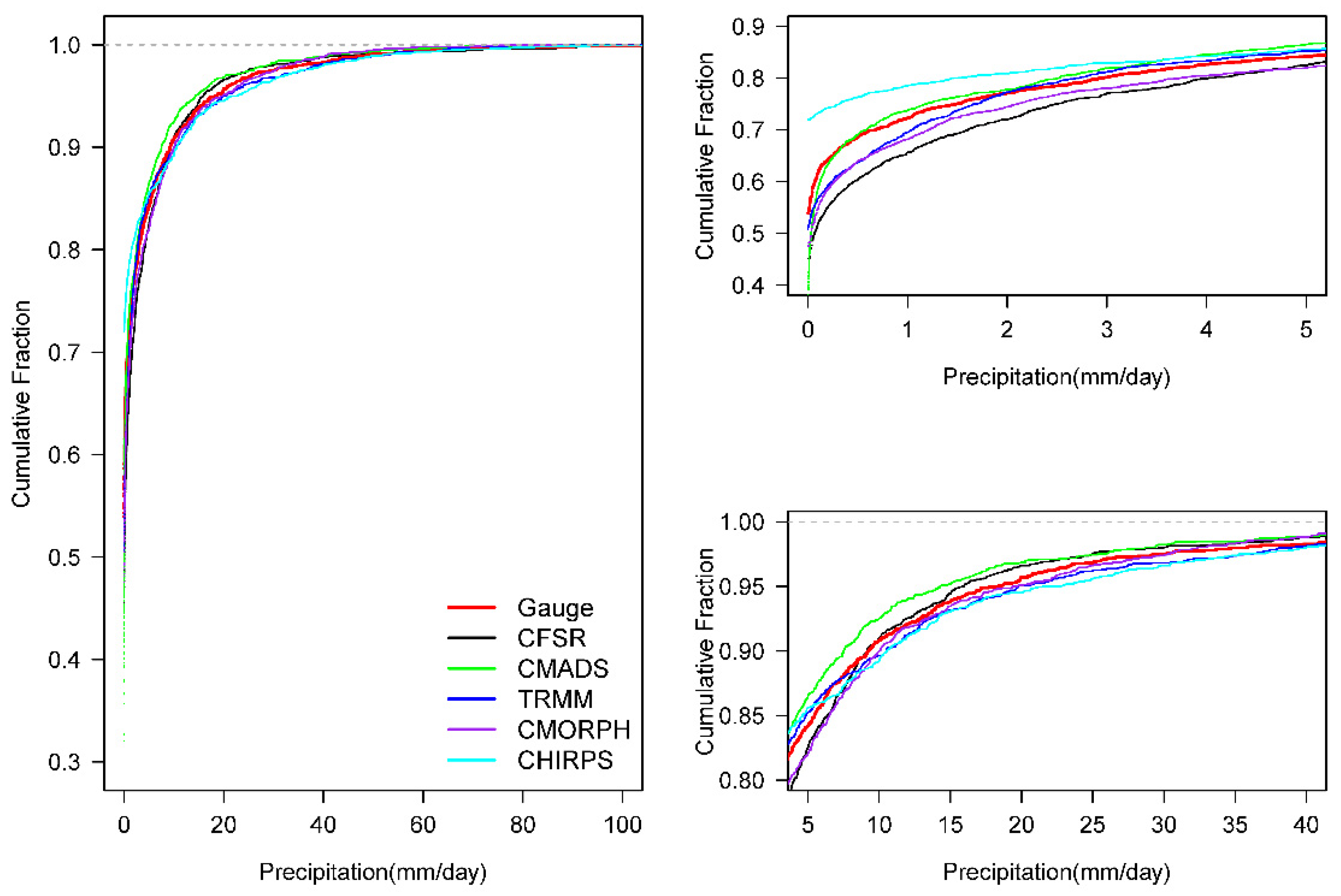
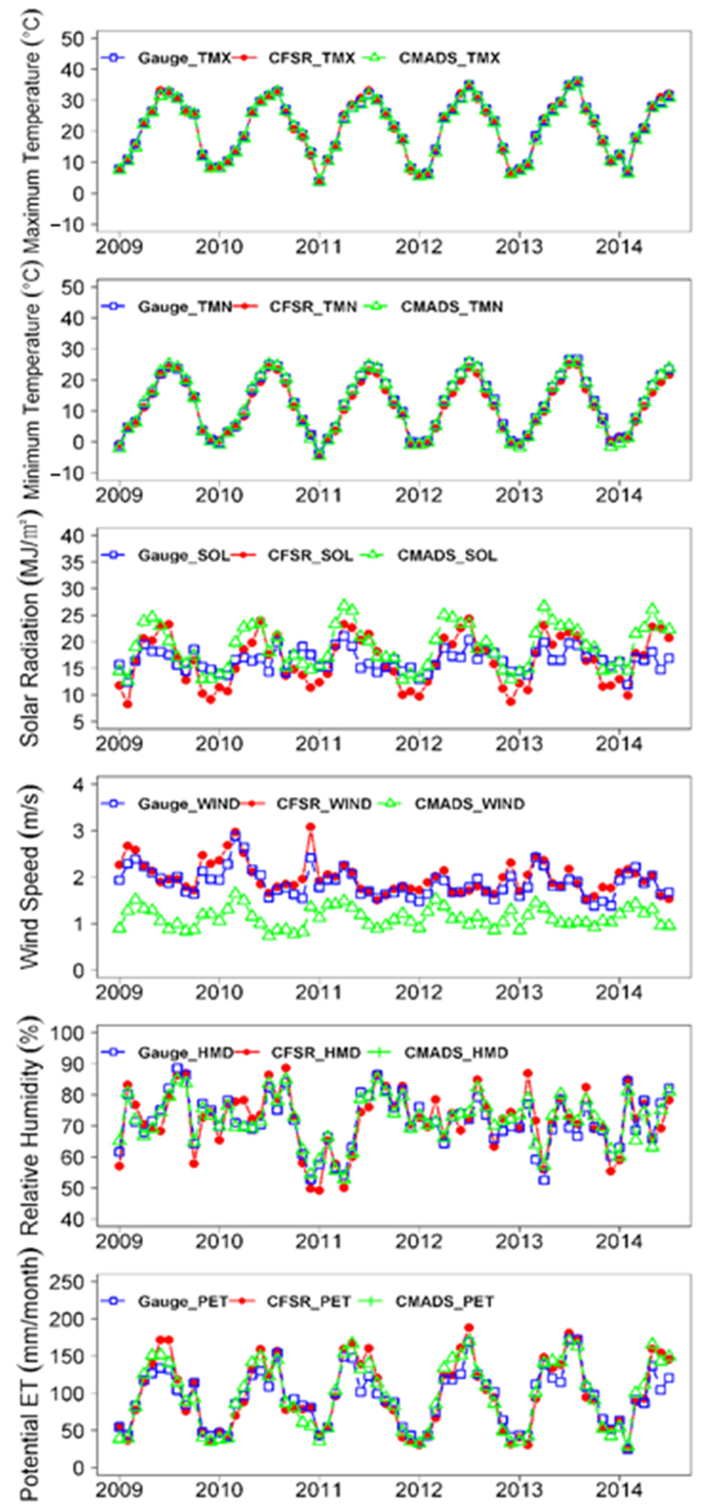
In this study area, the three satellite-based precipitation datasets (i.e., TRMM, CMORPH, and CHIRPS) were generally close to gauged data except for some lower peaks, while CMADS had overall lower precipitation than gauged data and CFSR had poor temporal consistency with gauged data. For the other meteorological variables, excluding precipitation, CFSR and CMADS had fairly good agreement with gauged data in the maximum temperature, minimum temperature, and relative humidity, but there are large discrepancies among them for the solar radiation and wind speed. In particular, for solar radiation, gauged data had smaller fluctuations than the other two datasets; for wind speed, CMADS was considerably lower than the gauged and CFSR datasets. However, despite these discrepancies, overall monthly PET totals from the three datasets were in good agreement, suggesting that the discrepancies in individual weather variables cancelled each other to a certain degree.
(2)
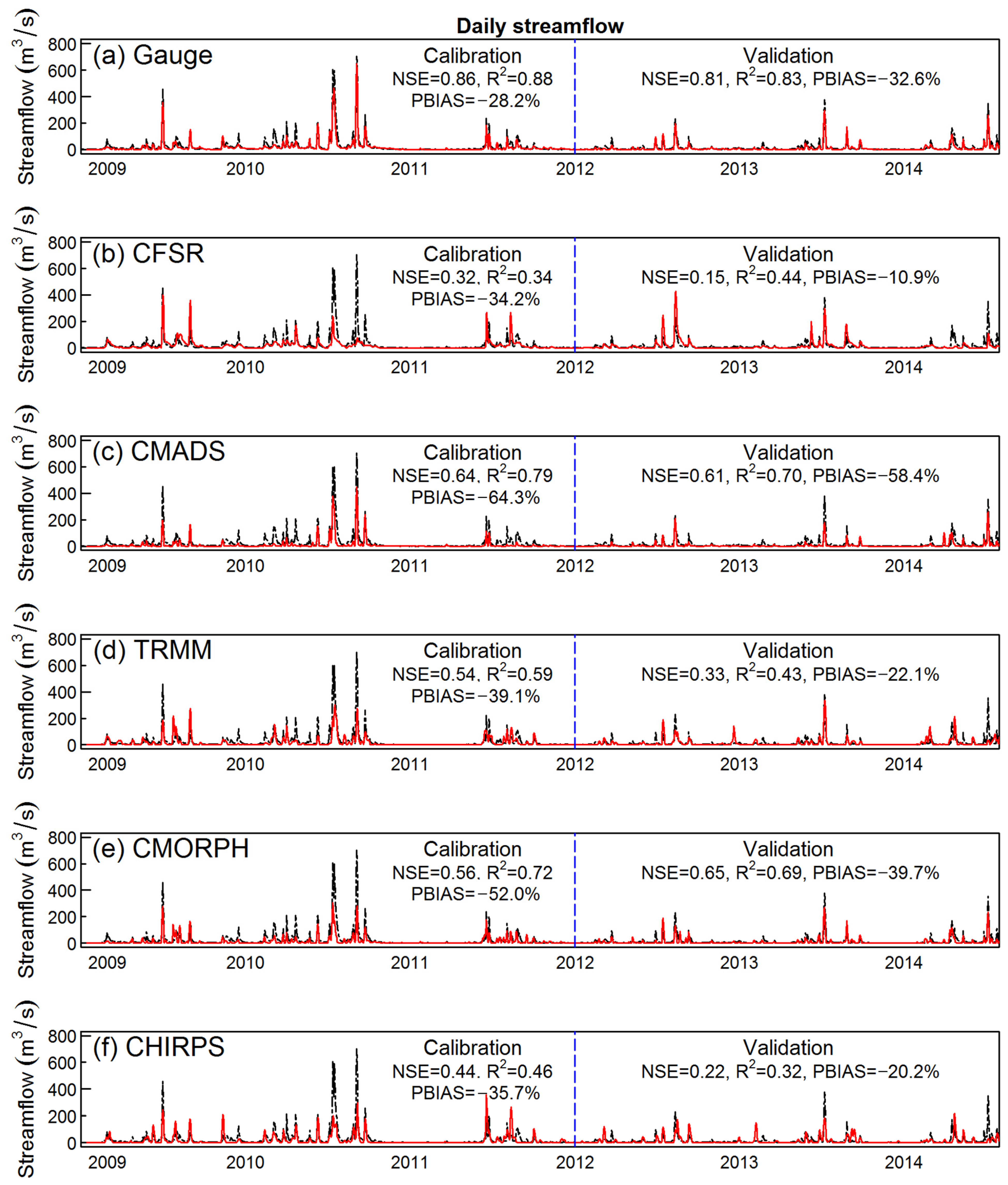
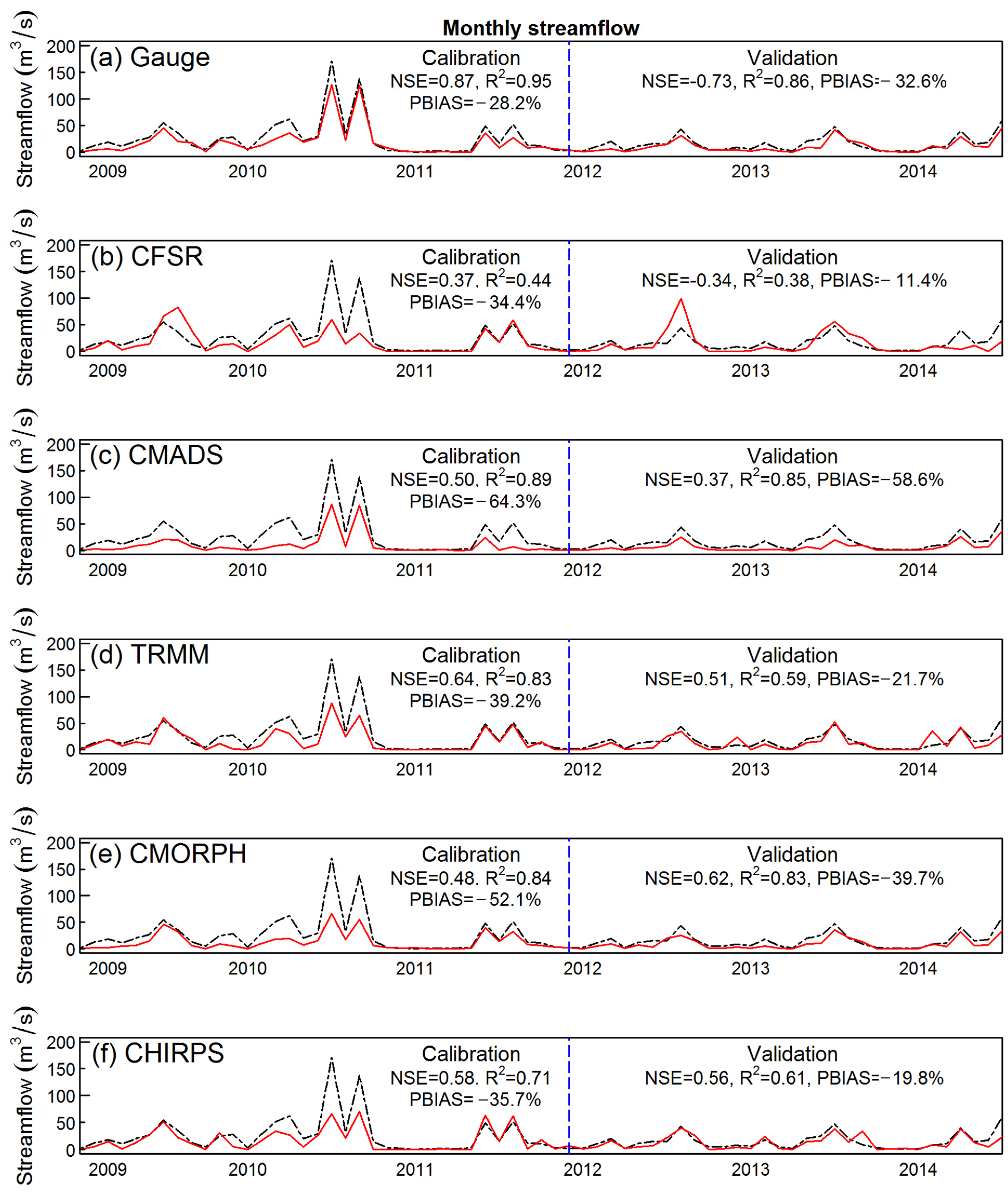
The impact of precipitation data on simulated streamflow is much larger than that of other meteorological data. In this study, the best simulation results were obtained using gauged data for both precipitation and other meteorological variables. At the same time, this study also got satisfactory daily simulation results using the CMORPH precipitation data and monthly simulation results using the TRMM and CHIRPS precipitation data. These results suggested that different gridded precipitation datasets should be used to obtain optimal results for daily and monthly streamflow simulations. Although the models using different meteorological datasets had comparable performance, CFSR usually performed better than CMADS especially at the monthly scale in this area.
(3)
There were considerable differences in the calibrated optimal parameters and water balance components among the eighteen scenarios even for the scenarios with similar water yield to streamflow (e.g., the scenarios using gauged precipitation data and those using CFSR precipitation data). This highlights the inherent limitations of model calibration only based on measured streamflow at the outlet, which should be reduced through multivariable and multisite calibration once data allows.
Currently, the development of data fusion and machine learning techniques provides unprecedented opportunities to design novel methods to reduce the uncertainties of the precipitation dataset. While the focus of this study was to evaluate the performance of existing datasets on hydrological modeling, in the future, novel methods should be developed to construct more accurate precipitation datasets. In addition, it is important to obtain the right simulation results for the right reasons, especially for policy makers. Although the simulation results in this study were generally good based on indicators such as NSE and R2, the SWAT model did not adequately represent the impacts of widely distributed paddy fields and ditches on hydrological processes in this study area. In the future, the model should be improved to better characterize these agriculture-related processes and make the simulation results more reliable for decision making.

Supplementary Materials

The following supporting information can be downloaded at: https://www.mdpi.com/article/10.3390/w14091406/s1, Figure S1: Annual mean WYLD (water yield) for simulations using CFSR meteorological data and different precipitation data during 2009–2014, including (a) Gauge, (b) CFSR, (c) CMADS, (d) TRMM, (e) CMORPH, and (f) CHIRPS.

Author Contributions

Conceptualization, J.L. and Y.L.; methodology, J.L., L.Y. and Y.L.; software, J.L. and L.Y.; validation, L.Y.; formal analysis, J.L. and L.Y.; investigation, Y.Z. and L.Y.; resources, L.Y.; data curation, J.L. and L.Y.; writing—original draft preparation, J.L. and L.Y.; writing—review and editing, J.L., L.Y. and Y.L.; visualization, Y.Z. and L.Y.; supervision, Y.L.; project administration, Y.L.; funding acquisition, Y.L. All authors have read and agreed to the published version of the manuscript.

Funding

This research was funded by the National Natural Science Foundation of China (Project No.: 51879130 and 42077449), Discipline Innovation and Talent Introduction Base Project of Colleges and Universities in Henan Province of China (Project No.: CXJD2019001).

Institutional Review Board Statement

Not applicable.

Informed Consent Statement

Informed consent was obtained from all subjects involved in the study.

Data Availability Statement

The data used to support the findings of this study are included within the article.

Acknowledgments

We are thankful to the anonymous reviewers for their valuable comments.

Conflicts of Interest

The authors declare no conflict of interest.

References

  1. Duan, Z.; Chen, Q.; Chen, C.; Liu, J.; Gao, H.; Song, X.; Wei, M. Spatiotemporal analysis of nonlinear trends in precipitation over Germany during 1951–2013 from multiple observation-based gridded products. Int. J. Climatol. 2019, 39, 2120–2135. [Google Scholar] [CrossRef]
  2. Liu, J.; Duan, Z.; Jiang, J.; Zhu, A. Evaluation of three satellite precipitation products TRMM 3B42, CMORPH, and PERSIANN over a subtropical watershed in China. Adv. Meteorol. 2015, 2015, 151239. [Google Scholar] [CrossRef] [Green Version]
  3. Dai, Q.; Yang, Q.; Zhang, J.; Zhang, S. Impact of gauge representative error on a radar rainfall uncertainty model. J. Appl. Meteorol. Climatol. 2018, 57, 2769–2787. [Google Scholar] [CrossRef]
  4. Duan, Z.; Gao, H.; Ke, C. Estimation of lake outflow from the poorly gauged Lake Tana (Ethiopia) using satellite remote sensing data. Remote Sens. 2018, 10, 1060. [Google Scholar] [CrossRef] [Green Version]
  5. Tauro, F.; Selker, J.; Van De Giesen, N.; Abrate, T.; Uijlenhoet, R.; Porfiri, M.; Manfreda, S.; Caylor, K.; Moramarco, T.; Benveniste, J. Measurements and observations in the XXI century (MOXXI): Innovation and multi-disciplinarity to sense the hydrological cycle. Hydrol. Sci. J. 2018, 63, 169–196. [Google Scholar] [CrossRef] [Green Version]
  6. Cornes, R.C.; van der Schrier, G.; van den Besselaar, E.J.; Jones, P.D. An ensemble version of the E-OBS temperature and precipitation data sets. J. Geophys. Res. Atmos. 2018, 123, 9391–9409. [Google Scholar] [CrossRef] [Green Version]
  7. Duan, Z.; Liu, J.; Tuo, Y.; Chiogna, G.; Disse, M. Evaluation of eight high spatial resolution gridded precipitation products in Adige Basin (Italy) at multiple temporal and spatial scales. Sci. Total Environ. 2016, 573, 1536–1553. [Google Scholar] [CrossRef] [Green Version]
  8. Duan, Z.; Tuo, Y.; Liu, J.; Gao, H.; Song, X.; Zhang, Z.; Yang, L.; Mekonnen, D.F. Hydrological evaluation of open-access precipitation and air temperature datasets using SWAT in a poorly gauged basin in Ethiopia. J. Hydrol. 2019, 569, 612–626. [Google Scholar] [CrossRef] [Green Version]
  9. Harris, I.; Jones, P.D.; Osborn, T.J.; Lister, D.H. Updated high-resolution grids of monthly climatic observations–the CRU TS3. 10 Dataset. Int. J. Climatol. 2014, 34, 623–642. [Google Scholar] [CrossRef] [Green Version]
  10. Saha, S.; Moorthi, S.; Wu, X.; Wang, J.; Nadiga, S.; Tripp, P.; Behringer, D.; Hou, Y.-T.; Chuang, H.-Y.; Iredell, M. The NCEP climate forecast system version 2. J. Clim. 2014, 27, 2185–2208. [Google Scholar] [CrossRef]
  11. Tapiador, F.J.; Turk, F.J.; Petersen, W.; Hou, A.Y.; García-Ortega, E.; Machado, L.A.; Angelis, C.F.; Salio, P.; Kidd, C.; Huffman, G.J. Global precipitation measurement: Methods, datasets and applications. Atmos. Res. 2012, 104, 70–97. [Google Scholar] [CrossRef]
  12. Meng, X.; Wang, H.; Shi, C.; Wu, Y.; Ji, X. Establishment and evaluation of the China meteorological assimilation driving datasets for the SWAT model (CMADS). Water 2018, 10, 1555. [Google Scholar] [CrossRef] [Green Version]
  13. Arnold, J.G.; Moriasi, D.N.; Gassman, P.W.; Abbaspour, K.C.; White, M.J.; Srinivasan, R.; Santhi, C.; Harmel, R.; Van Griensven, A.; Van Liew, M.W. SWAT: Model use, calibration, and validation. Trans. ASABE 2012, 55, 1491–1508. [Google Scholar] [CrossRef]
  14. Cao, Y.; Zhang, J.; Yang, M.; Lei, X.; Guo, B.; Yang, L.; Zeng, Z.; Qu, J. Application of SWAT model with CMADS data to estimate hydrological elements and parameter uncertainty based on SUFI-2 algorithm in the Lijiang River Basin, China. Water 2018, 10, 742. [Google Scholar] [CrossRef] [Green Version]
  15. Chen, M.; Yue, S.; Lü, G.; Lin, H.; Yang, C.; Wen, Y.; Hou, T.; Xiao, D.; Jiang, H. Teamwork-oriented integrated modeling method for geo-problem solving. Environ. Model. Softw. 2019, 119, 111–123. [Google Scholar] [CrossRef]
  16. Dile, Y.T.; Srinivasan, R. Evaluation of CFSR climate data for hydrologic prediction in data-scarce watersheds: An application in the Blue Nile River Basin. JAWRA J. Am. Water Resour. Assoc. 2014, 50, 1226–1241. [Google Scholar] [CrossRef]
  17. Liu, J.; Shanguan, D.; Liu, S.; Ding, Y. Evaluation and hydrological simulation of CMADS and CFSR reanalysis datasets in the Qinghai-Tibet Plateau. Water 2018, 10, 513. [Google Scholar] [CrossRef] [Green Version]
  18. Huffman, G.J.; Bolvin, D.T.; Nelkin, E.J.; Wolff, D.B.; Adler, R.F.; Gu, G.; Hong, Y.; Bowman, K.P.; Stocker, E.F. The TRMM multisatellite precipitation analysis (TMPA): Quasi-global, multiyear, combined-sensor precipitation estimates at fine scales. J. Hydrometeorol. 2007, 8, 38–55. [Google Scholar] [CrossRef]
  19. Fuka, D.R.; Walter, M.T.; MacAlister, C.; Degaetano, A.T.; Steenhuis, T.S.; Easton, Z.M. Using the climate forecast system reanalysis as weather input data for watershed models. Hydrol. Process. 2014, 28, 5613–5623. [Google Scholar] [CrossRef]
  20. Reichstein, M.; Camps-Valls, G.; Stevens, B.; Jung, M.; Denzler, J.; Carvalhais, N. Prabhat. Deep learning and process understanding for data-driven earth system science. Nature 2019, 566, 195–204. [Google Scholar] [CrossRef]
  21. Moraux, A.; Dewitte, S.; Cornelis, B.; Munteanu, A. A deep learning multimodal method for precipitation estimation. Remote Sens. 2021, 13, 3278. [Google Scholar] [CrossRef]
  22. Gilewski, P.; Nawalany, M. Inter-comparison of rain-gauge, radar, and satellite (IMERG GPM) precipitation estimates performance for rainfall-runoff modeling in a mountainous catchment in Poland. Water 2018, 10, 1665. [Google Scholar] [CrossRef] [Green Version]
  23. Sapountzis, M.; Kastridis, A.; Kazamias, A.; Karagiannidis, A.; Nikopoulos, P.; Lagouvardos, K. Utilization and uncertainties of satellite precipitation data in flash flood hydrological analysis in ungauged watersheds. Glob. Nest J. 2021, 23, 388–399. [Google Scholar]
  24. Bitew, M.M.; Gebremichael, M.; Ghebremichael, L.T.; Bayissa, Y.A. Evaluation of high-resolution satellite rainfall products through streamflow simulation in a hydrological modeling of a small mountainous watershed in Ethiopia. J. Hydrometeorol. 2012, 13, 338–350. [Google Scholar] [CrossRef]
  25. Tuo, Y.; Duan, Z.; Disse, M.; Chiogna, G. Evaluation of precipitation input for SWAT modeling in Alpine catchment: A case study in the Adige river basin (Italy). Sci. Total Environ. 2016, 573, 66–82. [Google Scholar] [CrossRef] [Green Version]
  26. Gao, F.; Zhang, Y.; Chen, Q.; Wang, P.; Yang, H.; Yao, Y.; Cai, W. Comparison of two long-term and high-resolution satellite precipitation datasets in Xinjiang, China. Atmos. Res. 2018, 212, 150–157. [Google Scholar] [CrossRef]
  27. Mahmoud, M.T.; Hamouda, M.A.; Mohamed, M.M. Spatiotemporal evaluation of the GPM satellite precipitation products over the United Arab Emirates. Atmos. Res. 2019, 219, 200–212. [Google Scholar] [CrossRef]
  28. Radcliffe, D.; Mukundan, R. PRISM vs. CFSR precipitation data effects on calibration and validation of SWAT models. JAWRA J. Am. Water Resour. Assoc. 2017, 53, 89–100. [Google Scholar] [CrossRef]
  29. Zhang, L.; Meng, X.; Wang, H.; Yang, M. Simulated runoff and sediment yield responses to land-use change using the SWAT model in northeast China. Water 2019, 11, 915. [Google Scholar] [CrossRef] [Green Version]
  30. Zhu, Q.; Hsu, K.L.; Xu, Y.P.; Yang, T. Evaluation of a new satellite-based precipitation data set for climate studies in the Xiang River basin, southern China. Int. J. Climatol. 2017, 37, 4561–4575. [Google Scholar] [CrossRef]
  31. Jiang, S.; Liu, R.; Ren, L.; Wang, M.; Shi, J.; Zhong, F.; Duan, Z. Evaluation and hydrological application of CMADS reanalysis precipitation data against four satellite precipitation products in the Upper Huaihe River Basin, China. J. Meteorol. Res. 2020, 34, 1096–1113. [Google Scholar] [CrossRef]
  32. Yong, B.; Hong, Y.; Ren, L.L.; Gourley, J.J.; Huffman, G.J.; Chen, X.; Wang, W.; Khan, S.I. Assessment of evolving TRMM-based multisatellite real-time precipitation estimation methods and their impacts on hydrologic prediction in a high latitude basin. J. Geophys. Res. Atmos. 2012, 117, D09108. [Google Scholar] [CrossRef] [Green Version]
  33. Hu, S.; Qiu, H.; Yang, D.; Cao, M.; Song, J.; Wu, J.; Huang, C.; Gao, Y. Evaluation of the applicability of climate forecast system reanalysis weather data for hydrologic simulation: A case study in the Bahe River Basin of the Qinling Mountains, China. J. Geogr. Sci. 2017, 27, 546–564. [Google Scholar] [CrossRef] [Green Version]
  34. Yang, Y.; Wang, G.; Wang, L.; Yu, J.; Xu, Z. Evaluation of gridded precipitation data for driving SWAT model in area upstream of three gorges reservoir. PLoS ONE 2014, 9, e112725. [Google Scholar] [CrossRef]
  35. Li, Y.; Wang, Y.; Zheng, J.; Yang, M. Investigating spatial and temporal variation of hydrological processes in western China driven by CMADS. Water 2019, 11, 435. [Google Scholar] [CrossRef] [Green Version]
  36. Zhang, Z.; Gao, J.; Gao, Y. The influences of land use changes on the value of ecosystem services in Chaohu Lake Basin, China. Environ. Earth Sci. 2015, 74, 385–395. [Google Scholar] [CrossRef]
  37. Liu, J.; Liu, Z.; Yin, Y.; Croke, B.F.W.; Chen, M.; Qin, C.-Z.; Tang, G.; Zhu, A.X. A hybrid vector-raster approach to drainage network construction in agricultural watersheds with rice terraces and ponds. J. Hydrol. 2021, 601, 126585. [Google Scholar] [CrossRef]
  38. Kong, X.; He, Q.; Yang, B.; He, W.; Xu, F.; Janssen, A.B.; Kuiper, J.J.; van Gerven, L.P.; Qin, N.; Jiang, Y. Hydrological regulation drives regime shifts: Evidence from paleolimnology and ecosystem modeling of a large shallow Chinese lake. Glob. Chang. Biol. 2017, 23, 737–754. [Google Scholar] [CrossRef]
  39. Meng, X.; Wang, H. Significance of the China meteorological assimilation driving datasets for the SWAT model (CMADS) of East Asia. Water 2017, 9, 765. [Google Scholar] [CrossRef]
  40. Xie, P.; Joyce, R.; Wu, S.; Yoo, S.-H.; Yarosh, Y.; Sun, F.; Lin, R. Reprocessed, bias-corrected CMORPH global high-resolution precipitation estimates from 1998. J. Hydrometeorol. 2017, 18, 1617–1641. [Google Scholar] [CrossRef]
  41. Arnold, J.G.; Srinivasan, R.; Muttiah, R.S.; Williams, J.R. Large area hydrologic modeling and assessment part I: Model development 1. JAWRA J. Am. Water Resour. Assoc. 1998, 34, 73–89. [Google Scholar] [CrossRef]
  42. Neitsch, S.L.; Arnold, J.G.; Kiniry, J.R.; Williams, J.R. Soil and Water Assessment Tool Theoretical Documentation Version 2009; Texas Water Resources Institute: College Station, TX, USA, 2011. [Google Scholar]
  43. Song, X.; Duan, Z.; Kono, Y.; Wang, M. Integration of remotely sensed C factor into SWAT for modelling sediment yield. Hydrol. Process. 2011, 25, 3387–3398. [Google Scholar] [CrossRef]
  44. Abbaspour, K.C.; Johnson, C.; Van Genuchten, M.T. Estimating uncertain flow and transport parameters using a sequential uncertainty fitting procedure. Vadose Zone J. 2004, 3, 1340–1352. [Google Scholar] [CrossRef]
  45. Abbaspour, K.C.; Yang, J.; Maximov, I.; Siber, R.; Bogner, K.; Mieleitner, J.; Zobrist, J.; Srinivasan, R. Modelling hydrology and water quality in the pre-alpine/alpine Thur watershed using SWAT. J. Hydrol. 2007, 333, 413–430. [Google Scholar] [CrossRef]
  46. Chow, V.T.; Maidment, D.R.; Mays, L.W. Applied Hydrology; McGraw-Hill Book Company: New York, NY, USA, 1988. [Google Scholar]
  47. Bredemeier, M.; Cohen, S.; Godbold, D.L.; Lode, E.; Pichler, V.; Schleppi, P. Forest Management and the Water Cycle: An Ecosystem-Based Approach; Springer Science & Business Media: Berlin/Heidelberg, Germany, 2010; Volume 212. [Google Scholar]
  48. Kastridis, A.; Theodosiou, G.; Fotiadis, G. Investigation of flood management and mitigation measures in ungauged NATURA protected watersheds. Hydrology 2021, 8, 170. [Google Scholar] [CrossRef]
  49. Schleppi, P. Forested water catchments in a changing environment. In Forest Management and the Water Cycle; Springer: Berlin/Heidelberg, Germany, 2010; pp. 89–110. [Google Scholar]
  50. Nash, J.E.; Sutcliffe, J.V. River flow forecasting through conceptual models part I—A discussion of principles. J. Hydrol. 1970, 10, 282–290. [Google Scholar] [CrossRef]
  51. Moriasi, D.N.; Arnold, J.G.; Van Liew, M.W.; Bingner, R.L.; Harmel, R.D.; Veith, T.L. Model evaluation guidelines for systematic quantification of accuracy in watershed simulations. Trans. ASABE 2007, 50, 885–900. [Google Scholar] [CrossRef]
  52. Peng, J.; Liu, T.; Huang, Y.; Ling, Y.; Li, Z.; Bao, A.; Chen, X.; Kurban, A.; De Maeyer, P. Satellite-based precipitation datasets evaluation using gauge observation and hydrological modeling in a typical arid land watershed of Central Asia. Remote Sens. 2021, 13, 221. [Google Scholar] [CrossRef]
  53. Bitew, M.M.; Gebremichael, M. Evaluation of satellite rainfall products through hydrologic simulation in a fully distributed hydrologic model. Water Resour. Res. 2011, 47, W06526. [Google Scholar] [CrossRef]
  54. Tan, M.L.; Gassman, P.W.; Liang, J.; Haywood, J.M. A review of alternative climate products for SWAT modelling: Sources, assessment and future directions. Sci. Total Environ. 2021, 795, 148915. [Google Scholar] [CrossRef]
  55. Zhang, D.; Tan, M.L.; Dawood, S.R.; Samat, N.; Chang, C.K.; Roy, R.; Tew, Y.L.; Mahamud, M.A. Comparison of NCEP-CFSR and CMADS for hydrological modelling using SWAT in the Muda River Basin, Malaysia. Water 2020, 12, 3288. [Google Scholar] [CrossRef]
  56. Gao, X.; Zhu, Q.; Yang, Z.; Wang, H. Evaluation and hydrological application of CMADS against TRMM 3B42V7, PERSIANN-CDR, NCEP-CFSR, and gauge-based datasets in Xiang River Basin of China. Water 2018, 10, 1225. [Google Scholar] [CrossRef] [Green Version]
  57. Chua, Z.-W.; Kuleshov, Y.; Watkins, A. Evaluation of satellite precipitation estimates over Australia. Remote Sens. 2020, 12, 678. [Google Scholar] [CrossRef] [Green Version]
  58. Yang, W.-T.; Fu, S.-M.; Sun, J.-H.; Zheng, F.; Wei, J.; Ma, Z. Comparative evaluation of the performances of TRMM-3B42 and climate prediction centre morphing technique (CMORPH) precipitation estimates over Thailand. J. Meteorol. Soc. Jpn. Ser. II 2021, 99, 1525–1546. [Google Scholar] [CrossRef]
  59. Darbandsari, P.; Coulibaly, P. Inter-comparison of lumped hydrological models in data-scarce watersheds using different precipitation forcing data sets: Case study of Northern Ontario, Canada. J. Hydrol. Reg. Stud. 2020, 31, 100730. [Google Scholar] [CrossRef]
  60. Kumari, N.; Srivastava, A.; Sahoo, B.; Raghuwanshi, N.S.; Bretreger, D. Identification of suitable hydrological models for streamflow assessment in the Kangsabati River Basin, India, by using different model selection scores. Nat. Resour. Res. 2021, 30, 4187–4205. [Google Scholar] [CrossRef]
  61. Pappenberger, F.; Beven, K.J. Ignorance is bliss: Or seven reasons not to use uncertainty analysis. Water Resour. Res. 2006, 42, W05302. [Google Scholar] [CrossRef]
  62. Beven, K.; Binley, A. The future of distributed models: Model calibration and uncertainty prediction. Hydrol. Process. 1992, 6, 279–298. [Google Scholar] [CrossRef]
  63. Vrugt, J.A.; ter Braak, C.J.F.; Diks, C.G.H.; Robinson, B.A.; Hyman, J.M.; Higdon, D. Accelerating markov chain monte carlo simulation by differential evolution with self-adaptive randomized subspace sampling. Int. J. Nonlinear Sci. Numer. Simul. 2009, 10, 273–290. [Google Scholar] [CrossRef]
  64. Refsgaard, J.C.; Madsen, H.; Andréassian, V.; Arnbjerg-Nielsen, K.; Davidson, T.A.; Drews, M.; Hamilton, D.P.; Jeppesen, E.; Kjellström, E.; Olesen, J.E.; et al. A framework for testing the ability of models to project climate change and its impacts. Clim. Chang. 2014, 122, 271–282. [Google Scholar] [CrossRef] [Green Version]
Figure 1. Locations of the Fengle river basin, gauge stations, and the center points of grid cells of the gridded meteorological and precipitation datasets.
Water 14 01406 g001
Figure 2. Flowchart of streamflow simulation driven by open-access gridded meteorological and remote sensing precipitation products.
Water 14 01406 g002
Figure 3. The cumulative fraction of daily precipitation from six datasets (Gauge, CFSR, CMADS, TRMM, CMORPH, and CHIRPS) at the watershed scale during 2009–2014. The left subfigure shows the cumulative fraction for daily precipitation ranging from 0 to 100 mm/day; in order to show more details, the two subfigures in the right show the cumulative fraction for daily precipitation ranging from 0 to 5 mm/day and 5 to 40 mm/day, respectively.
Water 14 01406 g003
Figure 4. Comparison of monthly precipitation totals from six datasets at the watershed scale during 2009–2014, including (a) Gauge CFSR, and CMADS, (b) Gauge, TRMM, CMORPH, and CHIRPS.
Water 14 01406 g004
Figure 5. The cumulative fraction of daily maximum and minimum air temperature, solar radiation, wind speed, relative humidity, and potential ET from three different datasets (Gauge, CFSR, and CMADS) at the watershed scale during 2009–2014.
Water 14 01406 g005
Figure 6. Comparison of the monthly mean of daily maximum (TMX) and minimum (TMN) air temperature, solar radiation (SOL), wind speed (WIND), and relative humidity (HMD) from the Gauge, CFSR, and CMADS datasets, and their resulting potential evapotranspiration (PET) estimates at the watershed scale during 2009–2014.
Water 14 01406 g006
Figure 7. Comparison of daily measured (black line) and simulated (red line) streamflow from models using the CFSR meteorological (excluding precipitation) datasets and six different precipitation datasets for the period 2009–2014, including (a) Gauge, (b) CFSR, (c) CMADS, (d) TRMM, (e) CMORPH, and (f) CHIRPS.
Water 14 01406 g007
Figure 8. Comparison of monthly measured (black line) and simulated (red line) streamflow from models using the CFSR meteorological (excluding precipitation) datasets and six different precipitation datasets for the period 2009–2014, including (a) Gauge, (b) CFSR, (c) CMADS, (d) TRMM, (e) CMORPH, and (f) CHIRPS.
Water 14 01406 g008
Figure 9. Annual mean water balance components for simulations using eighteen scenarios during 2009–2014. The different colors represent using different precipitation datasets (Gauge, CFSR, CMADS, TRMM, CMORPH, CHIRPS), and the three bars displayed in the same color used the Gauge, CFSR, and CMADS meteorological data from left to right, respectively. AET—actual evapotranspiration; WYLD—water yield, the net amount of water that leaves the subbasin and contributes to streamflow in the reach; SUR_Q—surface runoff contribution to streamflow; GW_Q—groundwater contribution to streamflow; LAT_Q—lateral flow contribution to streamflow; PERC—water percolating past the root zone.
Water 14 01406 g009
Figure 10. Spatial distributions of annual mean precipitation using different precipitation data during 2009–2014, including (a) Gauge, (b) CFSR, (c) CMADS, (d) TRMM, (e) CMORPH, and (f) CHIRPS.
Water 14 01406 g010
Table 1. List of parameters used for calibration and their default values and ranges for calibration (“a__”, “v__”, and “r__” mean an absolute increase, a replacement, and a relative change from the initial parameter values, respectively).
ParametersDescriptionDefaultRange
v_ALPHA_BF.gwBaseflow alpha factor (1/days)0.0480–1
v_GW_DELAY.gwGroundwater delay [days]310–500
v_GW_REVAP.gwGroundwater “revap” coefficient0.020.02–0.2
v_ALPHA_BNK.rteBaseflow alpha factor for bank storage (days)00–1
v_CH_K2.rteEffective hydraulic conductivity [mm/hr]05–130
v_CH_N2.rteManning’s “n” value for the main channel0.0140–0.3
r_SOL_AWC.solAvailable water capacity of the soil layer [mm H2O/mm soil]Soil layer specific±60%
r_SOL_BD.solMoist bulk density (Mg/m3 or g/cm3)Soil layer specific±60%
r_SOL_K.solSaturated hydraulic conductivity (mm/hr)Soil layer specific±60%
r_CN2.mgtSCS runoff curve numberHRU specific−30–10%
v_SFTMP.bsnSnowfall temperature (°C)1−5–5
r_SLSUBBSN.hruAverage slope length (m)HRU specific0–20%
Table 2. Evaluation statistics for the performance of eighteen scenarios in daily streamflow simulation.
Precipitation DataMeteorological Data
(Excluding Precipitation)
2009–2011
(Calibration)
2012–2014
(Validation)
NSER2PBIAS (%)NSER2PBIAS (%)
GaugeGauge0.870.88−23.00.820.83−24.1
CFSR0.860.88−28.20.810.83−32.6
CMADS0.850.88−29.40.790.83−38.1
CFSRGauge0.320.34−26.00.150.452.6
CFSR0.320.34−34.20.150.44−10.9
CMADS0.300.32−27.60.190.44−3.0
CMADSGauge0.640.79−63.80.650.72−55.8
CFSR0.640.79−64.30.610.70−58.4
CMADS0.640.79−63.50.640.72−58.0
TRMMGauge0.500.53−25.30.380.44−13.5
CFSR0.540.59−39.10.330.43−22.1
CMADS0.450.48−30.60.370.44−23.0
CMORPHGauge0.560.69−49.20.650.68−37.8
CFSR0.560.72−52.00.650.69−39.7
CMADS0.550.70−53.20.640.68−43.5
CHIRPSGauge0.400.42−34.70.210.30−22.7
CFSR0.440.46−35.70.220.32−20.2
CMADS0.380.40−37.00.210.29−27.8
Table 3. Evaluation statistics for the performance of eighteen scenarios in monthly streamflow simulation.
Precipitation DataMeteorological Data
(Excluding Precipitation)
2009–2011
(Calibration)
2012–2014
(Validation)
NSER2PBIAS (%)NSER2PBIAS (%)
GaugeGauge0.890.95−23.00.820.89−24.2
CFSR0.870.95−28.20.730.86−32.6
CMADS0.860.95−29.40.670.85−38.2
CFSRGauge0.400.44−26.2−0.400.422.2
CFSR0.370.44−34.4−0.340.38−11.4
CMADS0.360.41−27.7−0.380.39−3.4
CMADSGauge0.520.91-63.80.450.85−56.0
CFSR0.500.89−64.30.370.85−58.6
CMADS0.510.90−63.60.410.87−58.2
TRMMGauge0.610.73−25.40.580.61−13.1
CFSR0.640.83−39.20.510.59−21.7
CMADS0.590.72−30.80.540.60−22.7
CMORPHGauge0.490.80−49.30.670.85−37.9
CFSR0.480.84−52.10.620.83−39.7
CMADS0.450.81−53.30.570.82−43.6
CHIRPSGauge0.580.69−34.70.590.66−22.4
CFSR0.580.71−35.70.560.61−19.8
CMADS0.550.68−36.90.470.57−27.4
Table 4. Optimal parameters calibrated for the scenarios using the Gauge, CFSR, and CMADS precipitation data. The scenarios using the same precipitation data and different meteorological (excluding precipitation) data often had similar optimal parameters (with the different ones displayed in bold). “Gauge_P” represents using gauged precipitation data, “Gauge_M” represents using gauged meteorological data, and so on.
ParametersGauge_P and Gauge_MGauge_P and CFSR_MGauge_P and CMADS_MCFSR_P and Gauge_MCFSR_P and CFSR_MCFSR_P and CMADS_MCMADS_P and Gauge_MCMADS_P and CFSR_MCMADS_P and CMADS_M
r__CN2.mgt0.01810.01810.0181−0.1025−0.1025−0.10250.05180.05180.0518
v__ALPHA_BF.gw0.53500.53500.53500.52070.52070.52070.47360.47360.4736
v__GW_DELAY.gw65.583565.583565.58358.69588.69588.6958208.5404208.5404208.5404
v__GW_REVAP.gw0.09760.09760.09760.05500.05500.05500.05940.05940.0594
v__ALPHA_BNK.rte0.24120.24120.24120.32640.32640.32640.35530.35530.3553
v__CH_K2.rte6.31796.31796.31796.72846.72846.72846.80556.80556.80545
v__CH_N2.rte0.09120.09120.09120.07620.07620.07620.07660.07660.0766
r__SOL_AWC().sol−0.4144−0.4144−0.4144−0.7113−0.3789−0.7113−0.1629−0.2983−0.2983
r__SOL_BD().sol0.02040.02040.02040.54260.54260.5426−0.5752−0.5752−0.5752
r__SOL_K().sol−0.0827−0.0827−0.08270.51850.51850.51850.27550.27550.2755
v__SFTMP.bsn2.9753.84423.84420.10920.10920.10924.27584.27584.2758
r__SLSUBBSN.hru0.07610.07610.07610.11640.11640.11640.03610.03610.0361
Table 5. Optimal parameters calibrated for the scenarios using the TRMM, CMORPH, and CHIRPS precipitation data. The scenarios using the same precipitation data and different meteorological (excluding precipitation) data often had similar optimal parameters (with the different ones displayed in bold). “Gauge_P” represents using gauged precipitation data, “Gauge_M” represents using gauged meteorological data, and so on.
ParametersTRMM_P and Gauge_MTRMM_P and CFSR_MTRMM_P and CMADS_MCMORPH_P and Gauge_MCMORPH_P and CFSR_MCMORPH_P and CMADS_MCHIRPS_P and Gauge_MCHIRPS_P and CFSR_MCHIRPS_P and CMADS_M
r__CN2.mgt0.05800.00310.01810.06760.06760.06760.00060.00310.0006
v__ALPHA_BF.gw0.86540.69980.53500.87820.87820.87820.30260.69980.3026
v__GW_DELAY.gw154.72782.789265.5835318.0529318.0529318.05292.27072.78922.2707
v__GW_REVAP.gw0.04410.06940.09760.02500.02500.02500.07600.06940.0760
v__ALPHA_BNK.rte0.36620.38040.24120.65120.65120.65120.35250.38040.3525
v__CH_K2.rte5.35778.55116.31797.56577.56577.56578.63238.55118.6323
v__CH_N2.rte0.08970.09300.09160.08400.08400.08400.12520.09300.1252
r__SOL_AWC().sol0.00080.0062−0.41440.17180.17180.17180.18000.00620.1800
r__SOL_BD().sol0.47540.58610.02040.01060.01060.01060.00980.58610.0098
r__SOL_K().sol0.45480.5931−0.08270.51600.51600.51600.44550.59310.4455
v__SFTMP.bsn0.7148−3.43153.84423.47743.47743.47740.5679−3.43150.5679
r__SLSUBBSN.hru0.17330.12050.07600.09010.09010.09010.04640.12050.0464
Publisher’s Note: MDPI stays neutral with regard to jurisdictional claims in published maps and institutional affiliations.

