
Inferring Population Structure from Early Life Stage: The Case of the European Anchovy in the Sicilian and Maltese Shelves

 , , , , and
Abstract
:1. Introduction
2. Materials and Methods
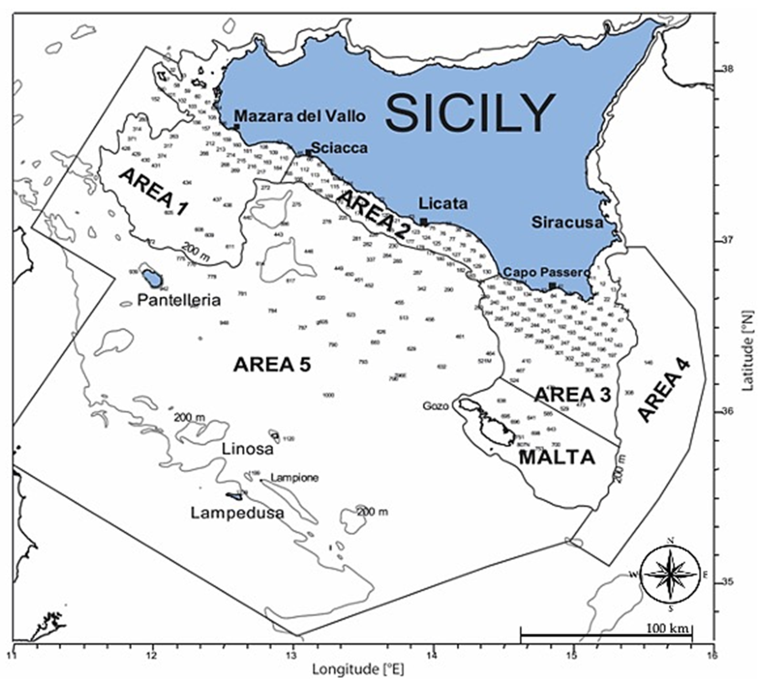
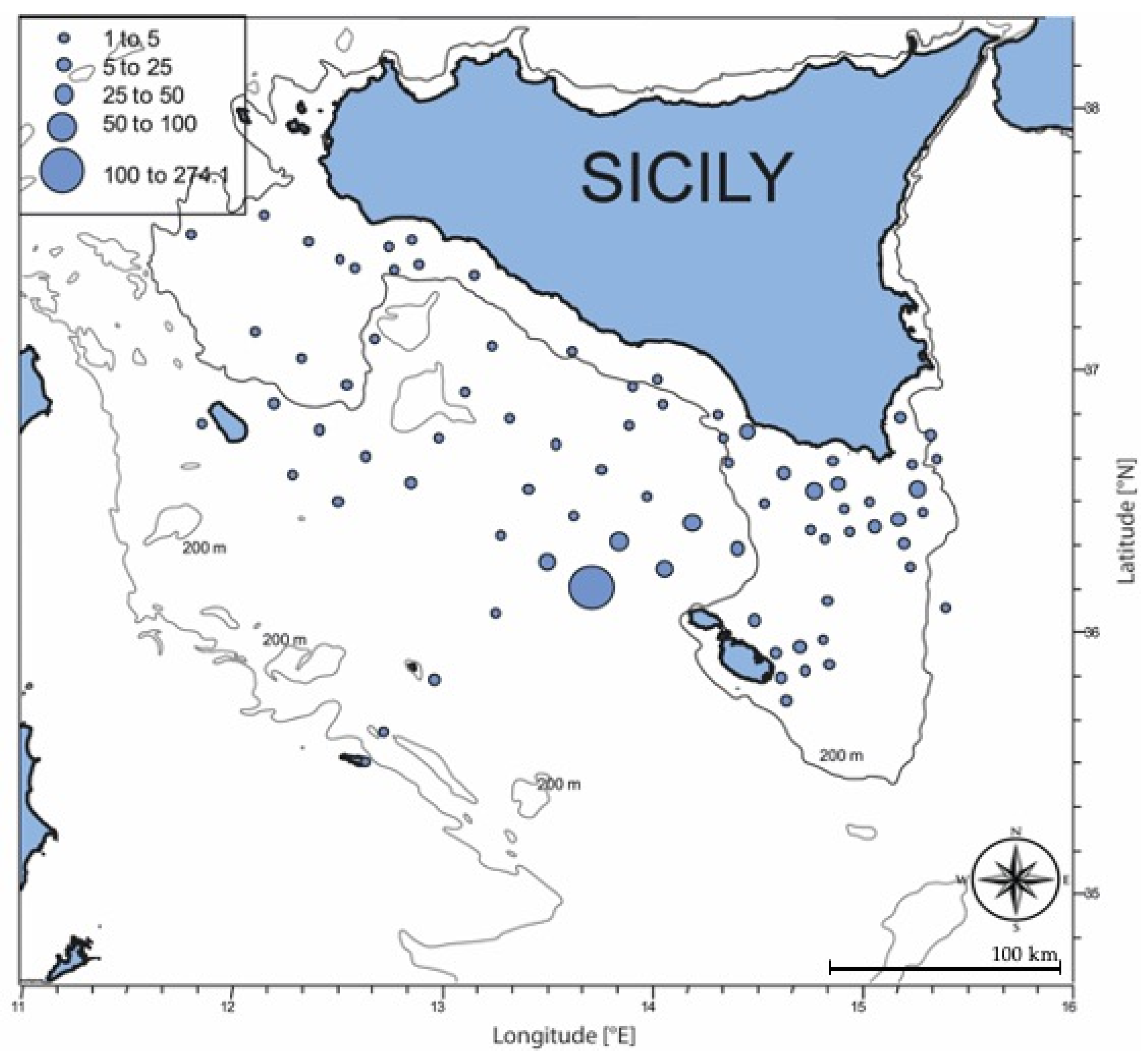
2.1. Sampling Area
2.2. Larval Sampling
2.3. Morphometric Analysis
2.4. Age Determination
2.5. Growth Rate Estimation
2.6. Larval Amino Acid Composition
2.7. Larval Organic Content
3. Results
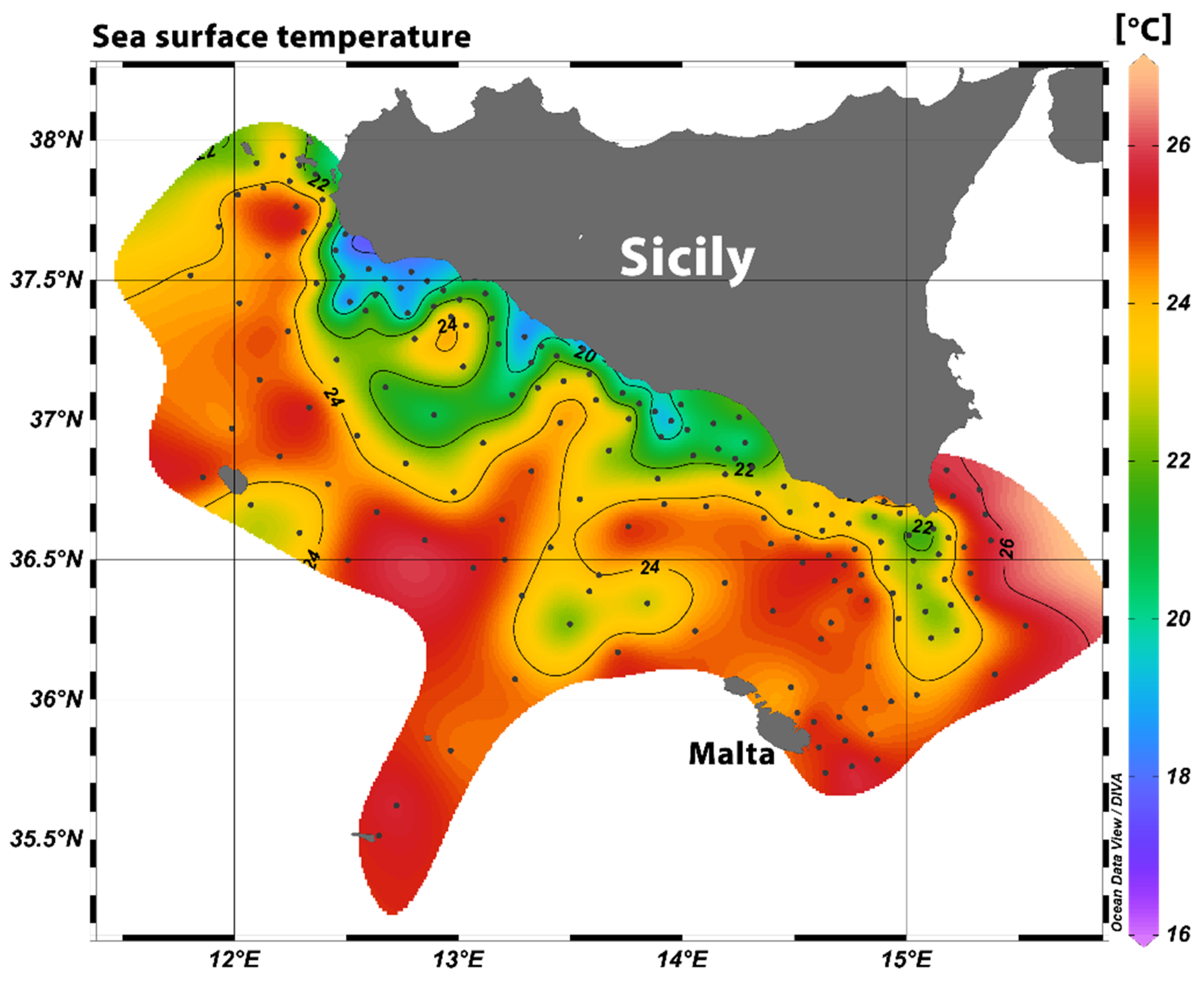
3.1. Oceanographic Conditions and Larval Density
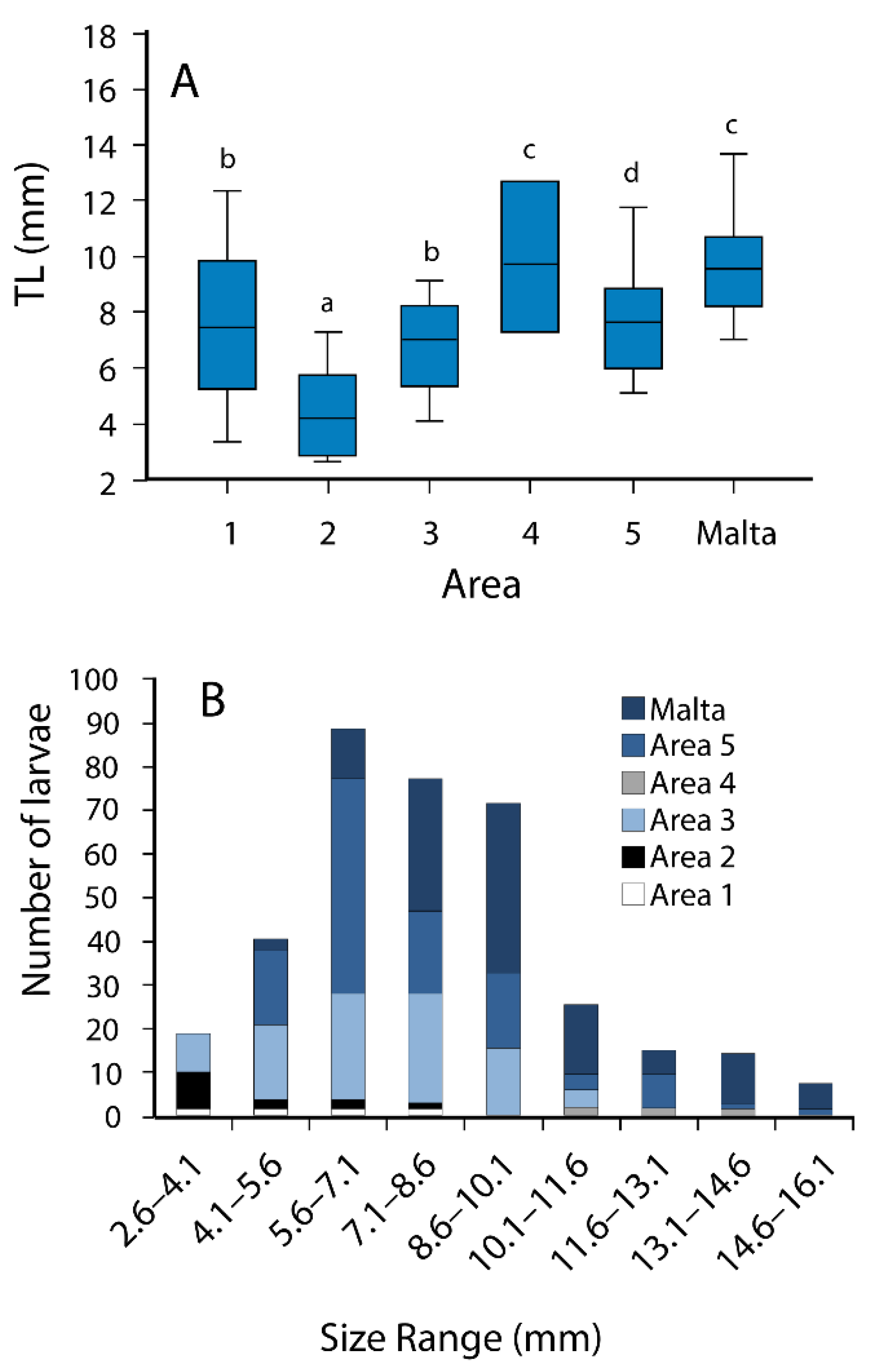
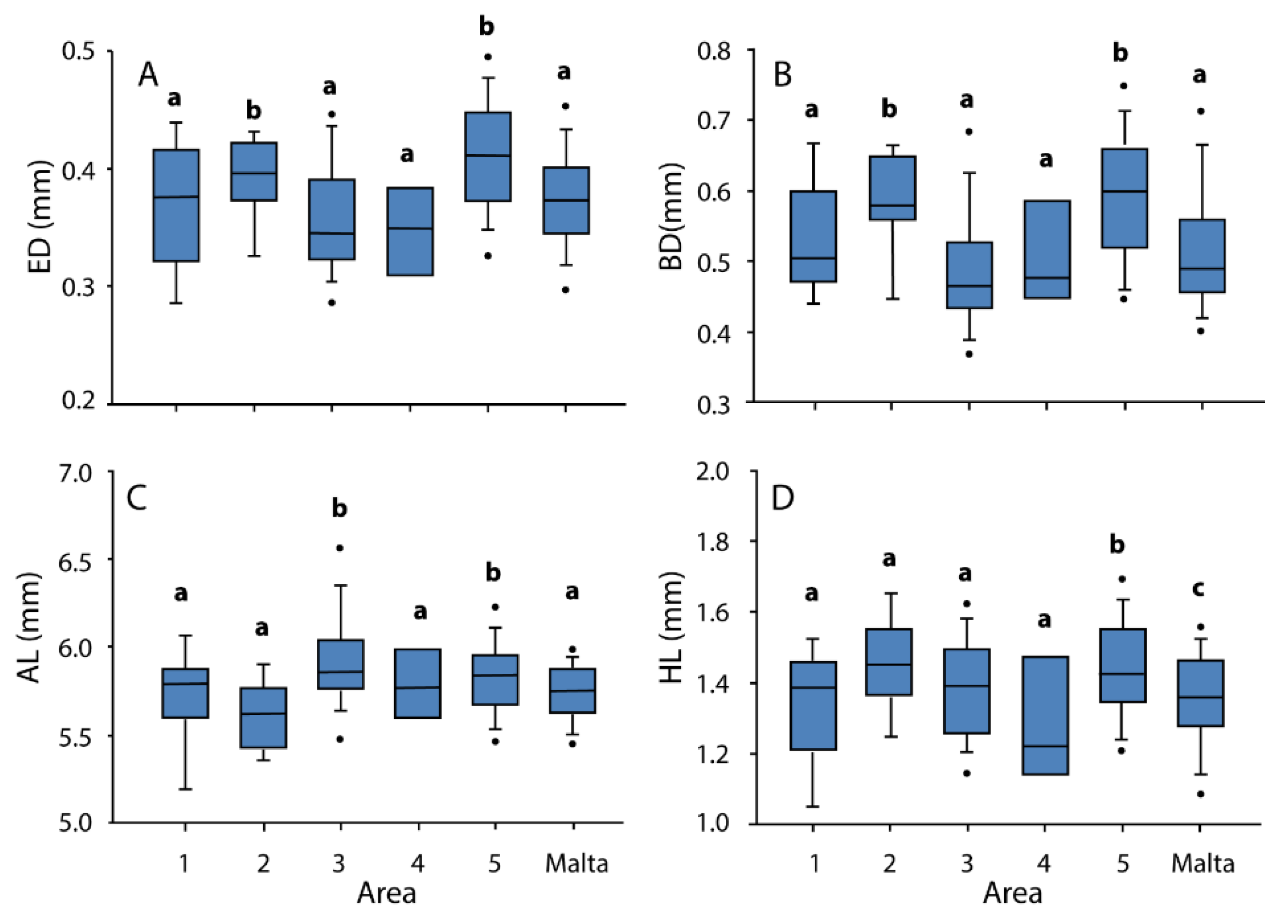
3.2. Morphometry
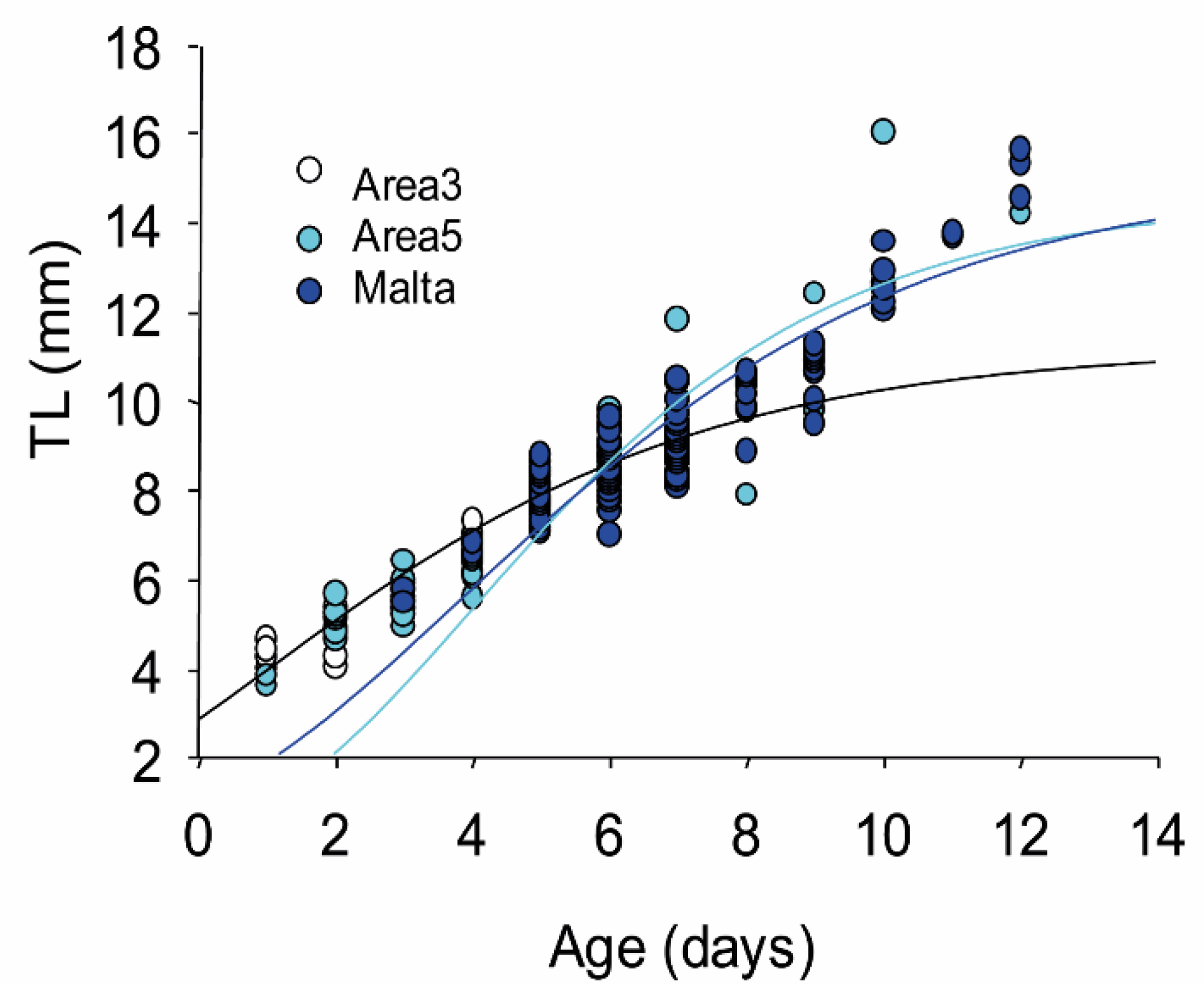
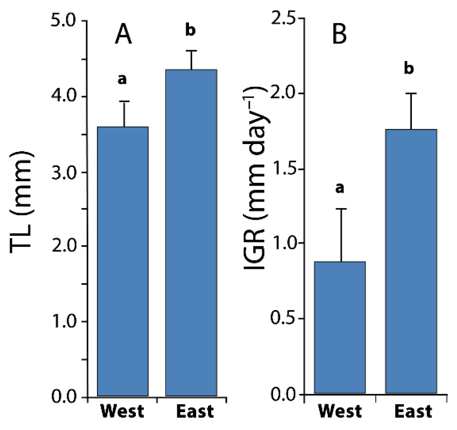
3.3. Larval Growth
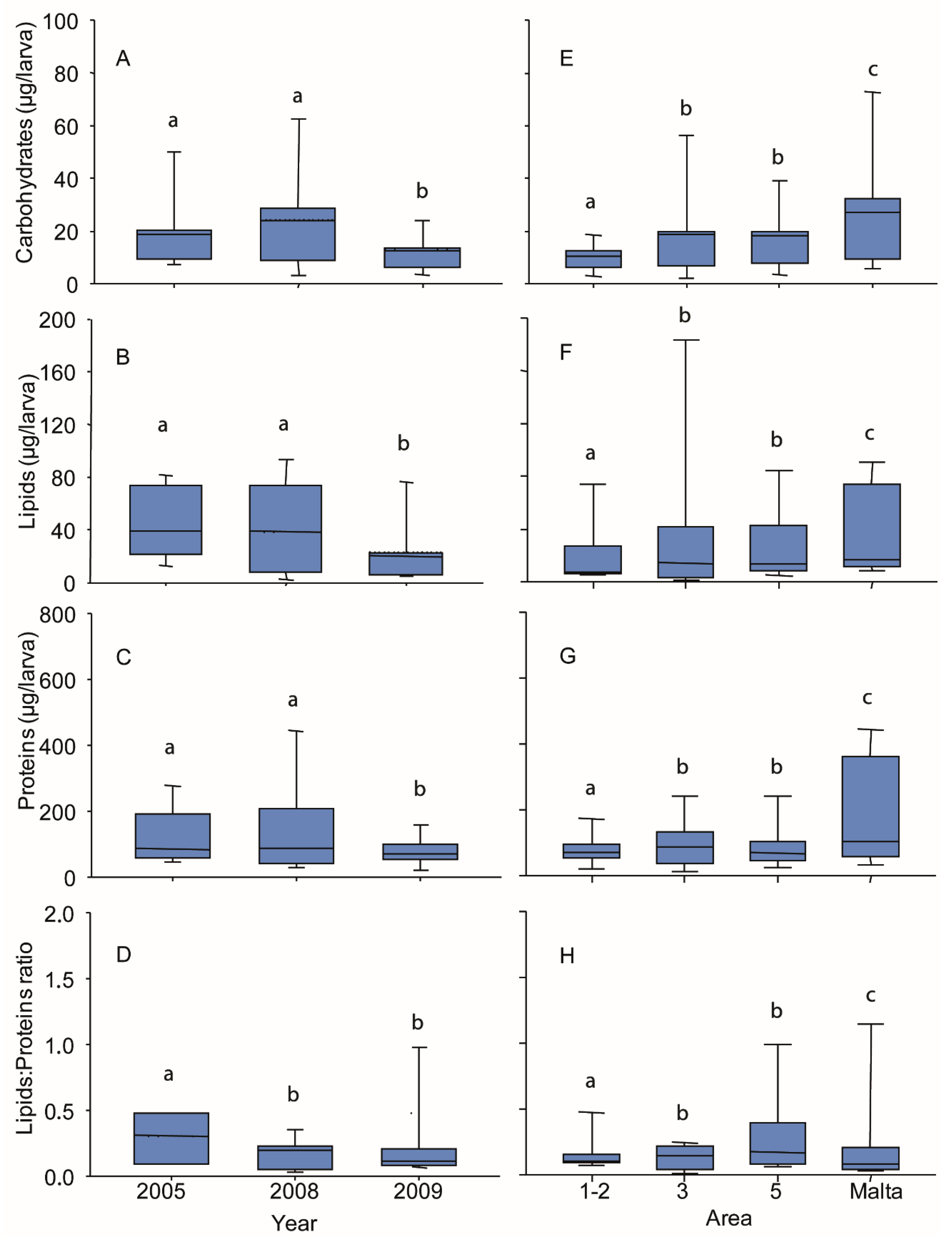
3.4. Biochemical Composition of Larvae
4. Discussion
Author Contributions
Funding
Institutional Review Board Statement
Informed Consent Statement
Data Availability Statement
Acknowledgments
Conflicts of Interest
References
- FAO. Review of the state of world marine Fishery resources. In FAO Fisheries and Aquaculture Technical Paper No. 569; FAO: Rome, Italy, 2011. [Google Scholar]
- SGMED; Study Group on Mediterranean Fisheries. Assessment of Mediterranean Stocks Part I; Scientific, Technical and Economic Committee for Fisheries (STECF): Luxembourg; Publications Office of the European Union: Heraklion, Crete, Greece, 2010. [Google Scholar]
- Cuttitta, A.; Guisande, C.; Riveiro, I.; Maneiro, I.; Patti, B.; Vergara, A.; Basilone, G.; Bonanno, A.; Mazzola, S. Factors structuring reproductive habitat suitability of the European anchovy (Engraulis encrasicolus) in the south coast of Sicily. J. Fish Biol. 2006, 67, 1–12. [Google Scholar]
- Fréon, P.; Cury, P.; Shannon, L.; Roy, C. Sustainable exploitation of small pelagic fish stocks challenged by environmental and ecosystem changes. Bull. Mar. Sci. 2005, 76, 385–462. [Google Scholar]
- Borja, Á.; Fontán, A.; Sáenz, J.; Valencia, V. Climate, oceanography, and recruitment: The case of the Bay of Biscay anchovy (Engraulis encrasicolus). Fish. Oceanogr. 2008, 17, 477–493. [Google Scholar] [CrossRef]
- Cuttitta, A.; Torri, M.; Zarrad, R.; Zgozi, S.; Jarboui, O.; Quinci, E.M.; Patti, B. Linking surface hydrodynamics to planktonic ecosystem: The case study of the ichthyoplanktonic assemblages in the Central Mediterranean Sea. Hydrobiologia 2018, 821, 191–214. [Google Scholar] [CrossRef]
- Bakun, A. Patterns in the Ocean: Ocean Processes and Marine Population Dynamics; University of California Sea Grant: San Diego, CA, USA, 1996; p. 323, (in cooperation with Centro de Investigaciones Biologicas de Noroeste, La Paz, Baja California Sur, Mexico). [Google Scholar]
- Takahashi, M.; Watanabe, Y. Effects of temperature and food availability on growth rate during late larval stage of Japanese anchovy (Engraulis japonicus) in the Kuroshio–Oyashio transition region. Fish. Oceanogr. 2005, 14, 223–235. [Google Scholar] [CrossRef]
- Palomera, I.; Olivar, M.P.; Salat, J.; Sabatés, A.; Coll, M.; García, A.; Morales-Nin, B. Small pelagic fish in the NW Mediterranean Sea: An ecological review. Prog. Oceanogr. 2007, 74, 377–396. [Google Scholar] [CrossRef]
- Houde, E.D. Emerging from Hjort’s shadow. J. Northwest Atl. Fish. Sci. 2008, 41, 53–70. [Google Scholar] [CrossRef]
- Bonanno, A.; Zgozi, S.; Cuttitta, A.; El Turki, A.; Di Nieri, A.; Ghmati, H.; Mazzola, S. Influence of environmental variability on anchovy early life stages (Engraulis encrasicolus) in two different areas of the Central Mediterranean Sea. Hydrobiology 2013, 701, 273–287. [Google Scholar] [CrossRef]
- Patti, B.; Torri, M.; Cuttitta, A. General surface circulation controls the interannual fluctuations of anchovy stock biomass in the Central Mediterranean Sea. Sci. Rep. 2020, 10, 1554. [Google Scholar] [CrossRef]
- Robinson, A.R.; Sellschopp, J.; Warn-Varnas, A.; Leslie, W.G.; Lozano, C.J.; Haley, P.J.J.; Lermusiaux, P.F.J. The Atlantic Ionian Stream. J. Mar. Syst. 1999, 20, 129–156. [Google Scholar] [CrossRef]
- Beranger, K.; Mortier, L.; Gasparini, G.P.; Gervasio, L.; Astraldi, M.; Crepon, M. The dynamics of the Strait of Sicily: A comprehensive study from observations and models. Deep-Sea Res. 2004, 51, 411–440. [Google Scholar]
- Macedo-Soares, L.; Eiras-Garcia, C.A.; Santarosa-Freire, A.; Muelbert, S.H. Large-Scale Ichthyoplankton and Water Mass Distribution along the South Brazil Shelf. PLoS ONE 2014, 9, e91241. [Google Scholar] [CrossRef] [PubMed] [Green Version]
- Cuttitta, A.; Carini, V.; Patti, B.; Bonanno, A.; Basilone, G.; Mazzola, S.; Cavalcante, C. Anchovy egg and larval distribution in relation to biological and physical oceanography in the Strait of Sicily. Hydrobiology 2003, 503, 117–120. [Google Scholar] [CrossRef]
- Basilone, G.; Bonanno, A.; Patti, B.; Mazzola, S.; Barra, M.; Cuttitta, A.; McBride, R. Spawning site selection by European anchovy (Engraulis encrasicolus) in relation to oceanographic conditions in the Strait of Sicily. Fish. Oceanogr. 2013, 22, 309–323. [Google Scholar] [CrossRef]
- García-Lafuente, J.; Garcıa, A.; Mazzola, S.; Quintanilla, L.; Delgado, J.; Cuttita, A.; Patti, B. Hydrographic phenomena influencing early life stages of the Sicilian Channel anchovy. Fish. Oceanogr. 2002, 11, 31–44. [Google Scholar] [CrossRef] [Green Version]
- Falcini, F.; Corrado, R.; Torri, M.; Mangano, M.C.; Zarrad, R.; Di Cintio, A.; Lacorata, G. Seascape connectivity of European anchovy in the Central Mediterranean Sea revealed by weighted Lagrangian backtracking and bio-energetic modelling. Sci. Rep. 2020, 10, 18630. [Google Scholar] [CrossRef]
- Patti, B.; Zarrad, R.; Jarboui, O.; Cuttitta, A.; Basilone, G.; Aronica, S.; Mazzola, S. Anchovy (Engraulis encrasicolus) early life stages in the Central Mediterranean Sea: Connectivity issues emerging among adjacent sub-areas across the Strait of Sicily. Hydrobiologia 2018, 821, 25–40. [Google Scholar] [CrossRef]
- Stephenson, R.L. Stock complexity in fisheries management: A perspective of emerging issues related to population sub-units. Fish. Res. 1999, 43, 247–249. [Google Scholar] [CrossRef]
- Tzeng, T.D. Morphological variation between populations of spotted mackerel Scomber australasicus of Taiwan. Fish. Res. 2004, 68, 45–55. [Google Scholar] [CrossRef]
- Félix-Uraga, R.; Quiñonez-Velázquez, C.; Hill, K.T.; Gómez-Muñoz, V.M.; Melo-Barrera, F.N.; García-Franco, W. Pacific Sardine (Sardinops sagax) stock discrimination off the west coast of Baja California and southern California using otholith morphometry. CalCOFI Rep. 2005, 46, 113–121. [Google Scholar]
- García-Rodríguez, F.J.; García-Gasca, S.A.; De La Cruz-Agüeroa, J.; Cota-Gómeza, V.M. A study of the population structure of the Pacific sardine Sardinops sagax (Jenyns, 1842) in Mexico based on morphometric and genetic analysis. Fish. Res. 2011, 107, 169–176. [Google Scholar] [CrossRef]
- Traina, S.; Basilone, G.; Saborido-Rey, F.; Ferreri, R.; Quinci, E.; Masullo, T.; Mazzola, S. Assessing population structure of European Anchovy (Engraulis encrasicolus) in the Central Mediterranean by means of traditional morphometry. Adv. Oceanogr. Limnol. 2011, 22, 141–153. [Google Scholar] [CrossRef]
- Vergara-Solana, F.J.; García-Rodríguez, F.J.; La Cruz-Agüero, D. Comparing body and otolith shape for stock discrimination of Pacific sardine, Sardinops sagax Jenyns, 1842. J. Appl. Ichthyol. 2013, 29, 1241–1246. [Google Scholar] [CrossRef]
- Joensen, H.; Grahl-Nielsen, O. Distinction among North Atlantic cod Gadus morhua stocks by tissue fatty acid profiles. J. Fish Biol. 2014, 84, 1904–1925. [Google Scholar] [CrossRef] [PubMed]
- Riveiro, I.; Guisande, C.; Franco, C.; Lago de Lanzos, A.; Solá, A.; Maneiro, I.; Vergara, A.R. Egg and larval amino acid composition as indicators of niche resource partitioning in pelagic fish species. Mar. Ecol. Prog. Ser. 2003, 260, 252–262. [Google Scholar] [CrossRef] [Green Version]
- Tanner, S.E.; Pérez, M.; Presa, P.; Thorrold, S.R.; Cabral, H.N. Integrating microsatellite DNA markers and otolith geochemistry to assess population structure of European hake (Merluccius merluccius). Est. Coast. Shelf. Sci. 2014, 142, 68–75. [Google Scholar] [CrossRef]
- Falco, F.; Barra, M.; Wu, G.; Dioguardi, M.; Stincone, P.; Cuttitta, A.; Cammarata, M. Engraulis encrasicolus larvae from two different environmental spawning areas of the Central Mediterranean Sea: First data on amino acid profiles and biochemical evaluations. Eur. Zool. J. 2020, 87, 580–590. [Google Scholar] [CrossRef]
- Abaunza, P.; Murta, A.G.; Campbell, N.; Cimmaruta, R.; Comesana, A.S.; Dahle, G.; Zimmermann, C. Stock identity of horse mackerel (Trachurus trachurus) in the Northeast Atlantic and Mediterranean Sea: Integrating the results from different stock identification approaches. Fish. Res. 2008, 89, 196–209. [Google Scholar] [CrossRef]
- Baibai, T.; Oukhattar, L.; Quinteiro, J.; Mesfioui, A.; Rey-Mendez, M.; Soukri, A. First global approach: Morphological and biological variability in a genetically homogeneous population of the European pilchard, Sardina pilchardus (Walbaum, 1792) in the North Atlantic coast. Rev. Fish Biol. Fish. 2012, 22, 63–80. [Google Scholar] [CrossRef]
- Zarraonaindia, I.; Iriondo, M.; Albaina, A.; Pardo, M.A.; Manzano, C.; Grant, W.S.; Irigoien, X.; Estonba, A. Multiple SNP markers reveal fine-scale population and deep phylogeographic structure in European anchovy (Engraulis encrasicolus L.). PLoS ONE 2012, 7, e42201. [Google Scholar] [CrossRef] [Green Version]
- Cuttitta, A.; Patti, B.; Maggio, T.; Quinci, E.; Pappalardo, A.; Ferrito, V.; De Pinto, V.; Mazzola, S. Larval population structure of Engraulis encrasicolus in the Strait of Sicily as revealed by morphometric and genetic analysis. Fish. Oceanogr. 2015, 24, 135–149. [Google Scholar] [CrossRef]
- Ryman, N.; Lagercrantz, U.; Andersson, L.; Chakraborty, R.; Rosenberg, R. Lack of correspondence between genetic and morphologic variability patterns in Atlantic herring. Heredity 1984, 53, 687–704. [Google Scholar] [CrossRef] [Green Version]
- Waldman, J.R. The importance of comparative studies in stock analysis. Fish. Res. 1999, 43, 237–246. [Google Scholar] [CrossRef]
- Ruggeri, P.; Splendiani, A.; Bonanomi, S.; Arneri, E.; Cingolani, N.; Santojanni, A.; Barucchi, V.C. Searching for a stock structure in Sardina pilchardus from the Adriatic and Ionian seas using a microsatellite DNA-based approach. Sci. Mar. 2013, 77, 565–574. [Google Scholar]
- Yaisel, J.B.; Piñera, J.A.; Sánchez Prado, J.A.; Blanco, G. Mitochondrial DNA and microsatellite genetic differentiation in the European anchovy Engraulis encrasicolus L. ICES J. Mar. Sci. 2012, 69, 1357–1371. [Google Scholar] [CrossRef] [Green Version]
- Turan, C.; Erguden, D.; Gurlek, M.; Basusta, N.; Turan, F. Morphometric structuring of the anchovy (Engraulis encrasicolus L.) in the Black, Aegean and northeastern Mediterranean Seas. Turk. J. Vet. Anim. Sci. 2004, 28, 865–871. [Google Scholar]
- Chang, M.Y.; Tzeng, W.N.; You, C.F. Using otolith trace elements as biological tracer for tracking larval dispersal of black porgy, Acanthopagrus schlegeli and yellowfin seabream, A. latus among estuaries of western Taiwan. Environ. Biol. Fish. 2012, 95, 491–502. [Google Scholar] [CrossRef]
- Cuttitta, A.; Basilone, G.; Patti, B.; Bonanno, A.; Mazzola, S.; Giusto, G.B. Trends in anchovy (Engraulis encrasicolus) condition factor and gonadosomatic index in the Sicilian Channel. Biol. Mar. Medit. 1999, 6, 566–568. [Google Scholar]
- Coombs, S.H.; Giovanardi, O.; Halliday, N.C.; Franceschini, G.; Conway, D.V.P.; Manzueto, L.; McFadzen, I.R.B. Wind mixing.; food availability and mortality of anchovy larvae Engraulis encrasicolus in the northern Adriatic Sea. Mar. Ecol. Prog. Ser. 2003, 248, 221–235. [Google Scholar] [CrossRef] [Green Version]
- Blackith, R.E.; Reyment, R.A. Multivariate Morphometrics; Academic Press: London, UK, 1971. [Google Scholar]
- Diaz, M.V.; Pájaro, M.; Sánchez, R.P. Employment of morphometric variables to assess nutritional condition of Argentine anchovy larvae Engraulis anchoita Hubbs & Marini., 1935. Rev. Biol Mar. Oceanogr. 2009, 44, 539–549. [Google Scholar]
- Sturges, H. The choice of a class-interval. J. Am. Stat. Assoc. 1926, 21, 65–66. [Google Scholar] [CrossRef]
- Lleonart, J.; Sarlat, J.; Torres, G.J. Removin allometric effects of body size morphological analysis. J. Theor. Biol. 2000, 205, 85–93. [Google Scholar] [CrossRef] [PubMed]
- Breiman, L. Random Forests. Mach. Learn. 2001, 45, 5–32. [Google Scholar] [CrossRef] [Green Version]
- Liaw, A.; Wiener, M. Classification and Regression by randomForest. R News 2002, 2, 18–22. [Google Scholar]
- Diaz-Uriarte, R.; Alvarez de Andres, S. Gene selection and classification of microarray data using random forest. BMC Bioinform. 2006, 7, 3. [Google Scholar] [CrossRef] [Green Version]
- Morales-Nin, B. Review of the growth regulation processes of otolith daily increment uniformation. Fish. Res. 2000, 46, 53–67. [Google Scholar] [CrossRef]
- Aldanondo, N.; Cotano, U.; Etxebeste, E.; Irigoien, X.; Álvarez, P.; Martínez de Murguía, A.; Herrero, D.L. Validation of daily increments deposition in the otoliths of European anchovy larvae (Engraulis encrasicolus L.) reared under different temperature. Fish. Res. 2008, 93, 257–264. [Google Scholar] [CrossRef]
- Zweifel, J.R.; Lasker, R. Prehatch and posthatch growth offishes—A general model. Fish. Bull. US 1976, 74, 609–621. [Google Scholar]
- Costalago, D.; Tecchio, S.; Palomera, I.; Alvarez-Calleja, I.; Ospina-Alvarez, A.; Raicevich, S. Ecological understanding for fishery management Condition and growth of anchovy late larvae during different seasons in the Northwestern Mediterranean. Estuar. Coast. Shelf Sci. 2011, 93, 350–358. [Google Scholar] [CrossRef] [Green Version]
- Regner, S. Ecology of planktonic stages of the anchovy, Engraulis encrasicolus (Linnaeus, 1758), in the Central Adriatic Sea. Acta Adriat. 1985, 26, 1–113. [Google Scholar]
- Ré, P. Ictioplâncton estuarino da Península Ibérica. In Guia de Identificação dos Ovos e Estados Larvares Planctónicos; Câmara Municipal de Cascais: Cascais, Portugal, 1999. [Google Scholar]
- Guisande, C.; Maneiro, I.; Riveiro, I. Homeostasis in the essential amino acid composition of the marine copepod Euterpina acutifrons. Limnol. Oceanogr. 1999, 44, 691–696. [Google Scholar] [CrossRef] [Green Version]
- Brucet, S.; Boix, D.; Lopez-Flores, R.; Badosa, A.; Quintana, X.D. Ontogenic changes of amino acid composition in planktonic crustacean species. Mar. Biol. 2005, 148, 131–139. [Google Scholar] [CrossRef]
- Lowry, O.H.; Rosenbraugh, N.J.; Farr, A.L.; Randall, R.J. Protein measurements with the Folin phenol reagent. J. Biol. Chem. 1951, 193, 256–275. [Google Scholar] [CrossRef]
- Maxwell, M.A.K.; Haas, S.M.; Bieber, L.L.; Tolbert, N.E. A modification of the Lowry procedure to simplify protein determination in membrane and lipoprotein samples. Anal. Biochem. 1978, 87, 206–210. [Google Scholar]
- Dubois, M.; Gilles, K.A.; Hamilton, J.K.; Smith, F. Colorimetric method for determination of sugars and related substances. Anal. Chem. 1956, 28, 350–356. [Google Scholar] [CrossRef]
- Zöllner, N.; Kirsch, K. Über die quantitative Bestimmung von Lipoiden (Mikromethode) mittels der vielen natürlichen Lipoiden (allen bekannten Plasmalipoiden) gemeinsamen Sulfophosphovanillin. Z. Gesamte Exp. Med. 1962, 135, 545–561. [Google Scholar] [CrossRef]
- Díaz, E.; Txurruka, J.M.; Villate, F. Biochemical composition and condition in anchovy larvae Engraulis encrasicolus during growth. Mar. Ecol. Prog. Ser. 2008, 361, 227–238. [Google Scholar] [CrossRef]
- Riveiro, I.; Guisande, C.; Maneiro, I.; Vergara, A.R. Parental effects in the European sardine Sardina pilchardus. Mar. Ecol. Prog. Ser. 2004, 274, 225–234. [Google Scholar] [CrossRef] [Green Version]
- Hasties, T.J.; Tibshirani, R.J. Generalized Additive MODELS; Chapman and Hall: New York, NY, USA, 1990. [Google Scholar]
- Wood, S.N. Generalized Additive Models: An Introduction with R; Chapman and Hall/CRC: New York, NY, USA, 2006. [Google Scholar]
- Sakamoto, Y.; Ishiguro, M.; Kitagawa, G. Akaike Information Criterion Statistics; D. Reidel: Dordrecht, The Netherlands, 1986; Volume 81, p. 26853. [Google Scholar]
- Cuttitta, A.; Quinci, E.M.; Patti, B.; Bonomo, S.; Bonanno, A.; Musco, M.; Mazzola, S. Different key roles of mesoscale oceanographic structures and ocean bathymetry in shaping larval fish distribution pattern: A case study in Sicilian waters in summer 2009. J. Sea Res. 2016, 115, 6–17. [Google Scholar] [CrossRef]
- Bonanno, A.; Placenti, F.; Basilone, G.; Mifsud, R.; Genovese, S.; Patti, B.; Mazzola, S. Variability of water mass properties in the Strait of Sicily in summer period of 1998–2013. Ocean Sci. 2014, 10, 759–770. [Google Scholar] [CrossRef] [Green Version]
- Torri, M.; Corrado, R.; Falcini, F.; Cuttitta, A.; Palatella, L.; Lacorata, G.; Santoleri, R. Planktonic stages of small pelagic fishes (Sardinella aurita and Engraulis encrasicolus) in the central Mediterranean Sea: The key role of physical forcings and implications for fisheries management. Prog. Oceanogr. 2018, 162, 25–39. [Google Scholar] [CrossRef]
- Falcini, F.; Palatella, L.; Cuttitta, A.; Buongiorno Nardelli, B.; Lacorata, G.; Lanotte, A.S.; Santoleri, R. The role of hydrodynamic processes on anchovy eggs and larvae distribution in the Sicily Channel (Mediterranean Sea): A case study for the 2004 data set. PLoS ONE 2015, 10, e0123213. [Google Scholar] [CrossRef] [PubMed]
- Cotano, U.; Irigoien, X.; Etxebeste, E.; Álvarez, P.; Zarauz, L.; Mader, J.; Ferrer, L. Distribution, growth and survival of anchovy larvae (Engraulis encrasicolus L.) in relation to hydrodynamic and trophic environment in the Bay of Biscay. J. Plankt. Res. 2008, 30, 467–481. [Google Scholar] [CrossRef] [Green Version]
- Heath, M.R. Field investigations of the early life stages of marine fish. Adv. Mar Biol. 1992, 28, 1–174. [Google Scholar]
- Diaz, M.V.; Arano, M.F.; Pájaro, M.; Aristizábal, E.O.; Macchi, G.F. The use of morphological and histological features as nutritional condition indices of Pagrus pagrus larvae. Neotrop. Ichthyol. 2013, 11, 649–660. [Google Scholar] [CrossRef] [Green Version]
- Yufera, M.; Polo, A.; Pascual, E. Changes in chemical composition and biomass during the transition from endogenous to exogenous feeding of Sparus aurata L. (Pisces.; Sparidae) larvae reared in the laboratory. J. Exp. Mar. Biol. Ecol. 1993, 167, 149–161. [Google Scholar] [CrossRef]
- Shan, X.J.; Cao, L.; Huang, W.; Dou, S.Z. Feeding, morphological changes and allometric growth during starvation in miiuy croaker larvae. Environ. Biol. Fish. 2009, 86, 121–130. [Google Scholar] [CrossRef]
- Bustos, C.; Silva, A. Endogenous feeding and morphological changes in hatchery-reared larval palm ruff Seriolella violacea (Pisces: Centrolophidae) under starvation. Aquac. Res. 2011, 42, 892–897. [Google Scholar] [CrossRef]
- Chambers, R.C. Environmental influences on egg and propagule sizes in marine fishes. In Early Life History and Recruitment in Fish Populations; Chambers, R.C., Trippel, E.A., Eds.; Chapman & Hall: London, UK, 1997; pp. 63–102. [Google Scholar]
- Castro, L.R.; Claramunt, G.; Krautz, M.C.; Llanos-Rivera, A.; Moreno, P. Egg trait variation in anchoveta Engraulis ringens: A maternal response to changing environmental conditions in contrasting spawning habitats. Mar. Ecol. Prog. Ser. 2009, 381, 237–248. [Google Scholar] [CrossRef] [Green Version]
- Schismenou, E.; Tsiaras, K.; Kourepini, M.I.; Lefkaditou, E.; Triantafyllou, G.; Somarakis, S. Seasonal changes in growth and condition of anchovy late larvae explained with a hydrodynamic-biogeochemical model simulation. Mar. Ecol. 2013, 478, 197–209. [Google Scholar] [CrossRef] [Green Version]
- Anderson, J.T. A review of size dependent survival during pre-recruit stages of fishes in relation to recruitment. J. Northwest Atl. Fish. Sci. 1988, 8, 55–66. [Google Scholar] [CrossRef]
- Ciechomski, J. The size of the egg of the Argentine anchovy Engraulis anchoita in relation to the season of the year of spawning. J. Fish Biol. 1973, 5, 393–398. [Google Scholar] [CrossRef]
- Gisbert, E.; Conklin, D.B.; Piedrahita, R.H. Effects of delayed first feeding on the nutritional condition and mortality of California halibut larvae. J. Fish Biol. 2004, 64, 116–132. [Google Scholar] [CrossRef]
- Torri, M.; Pappalardo, A.M.; Ferrito, V.; Giannì, S.; Armeri, G.M.; Patti, C.; Cuttitta, A. Signals from the deep-sea: Genetic structure, morphometric analysis, and ecological implications of Cyclothone braueri (Pisces, Gonostomatidae) early life stages in the Central Mediterranean Sea. Mar. Environ. Res. 2021, 169, 105379. [Google Scholar] [CrossRef]
- Catalán, I.A.; Berdalet, E.; Olivar, M.P.; Roldán, C. Response of muscle-based biochemical condition indices to short-term variations in food availability in postflexion reared sea bass Dicentrarchus labrax (L.) larvae. J. Fish Biol. 2007, 70, 391–405. [Google Scholar] [CrossRef]


| Temperature (°C) | Salinity (°/oo) | Fluorescence | |
|---|---|---|---|
| Area1 | 18.80 (±2.74) a | 37.69 (±0.16) | 0.034 (±0.008) |
| Area2 | 19.20 (±0.88) a | 37.64 (±0.12) | 0.028 (±0.005) |
| Area3 | 21.89 (±1.67) b | 37.64 (±0.23) | 0.026 (±0.005) |
| Area4 | 22.26 (±0.67) b | 38.17 (±0.25) | 0.034 (±0.004) |
| Area5 | 22.58 (±1.45) b | 37.52 (±0.14) | 0.028 (±0.004) |
| Malta | 24.49 (±0.31) c | 37.60 (±0.02) | 0.033 (±0.009) |
| Zone2 | Zone3 | Zone4 | Zone5 | Malta | ||||||||||||||||
|---|---|---|---|---|---|---|---|---|---|---|---|---|---|---|---|---|---|---|---|---|
| AL | HL | BD | ED | AL | HL | BD | ED | AL | HL | BD | ED | AL | HL | BD | ED | AL | HL | BD | ED | |
| Zone1 | - | - | - | - | ? | - | - | - | - | - | - | - | - | - | - | * | - | - | - | - |
| Zone2 | * | - | * | * | - | - | * | * | * | - | - | - | ? | ? | * | - | ||||
| Zone3 | - | - | - | - | ? | ? | * | * | * | - | - | * | ||||||||
| Zone4 | - | - | * | * | - | - | - | * | ||||||||||||
| Zone5 | * | * | * | * | ||||||||||||||||
| Number of Larvae Classified into Estimated Groups | ||||||||
|---|---|---|---|---|---|---|---|---|
| Area | 1 | 2 | 3 | 4 | 5 | Malta | % Correctly Classified | |
| Number of larvae classified into observed areas | 1 | 0 | 0 | 3 | 0 | 5 | 4 | 0 |
| 2 | 0 | 1 | 1 | 0 | 6 | 5 | 7.69 | |
| 3 | 0 | 0 | 48 | 0 | 21 | 24 | 51.62 | |
| 4 | 0 | 0 | 1 | 0 | 1 | 3 | 0 | |
| 5 | 1 | 1 | 16 | 0 | 72 | 29 | 60.5 | |
| Malta | 0 | 1 | 18 | 0 | 26 | 73 | 61.86 | |
| Number of Larvae Classified into Estimated Groups | ||||||||
|---|---|---|---|---|---|---|---|---|
| Area | 1 | 2 | 3 | 4 | 5 | Malta | % Correctly Classified | |
| Number of larvae classified into observed areas | 1 | 1 | 1 | 0 | 0 | 1 | 3 | 16.67 |
| 2 | 0 | 0 | 1 | 0 | 0 | 1 | 0 | |
| 3 | 0 | 1 | 5 | 0 | 1 | 6 | 38.46 | |
| 4 | 0 | 0 | 0 | 0 | 1 | 0 | 0 | |
| 5 | 0 | 0 | 0 | 0 | 39 | 2 | 95.12 | |
| Malta | 2 | 1 | 5 | 0 | 3 | 6 | 35.3 | |
Publisher’s Note: MDPI stays neutral with regard to jurisdictional claims in published maps and institutional affiliations. |
© 2022 by the authors. Licensee MDPI, Basel, Switzerland. This article is an open access article distributed under the terms and conditions of the Creative Commons Attribution (CC BY) license (https://creativecommons.org/licenses/by/4.0/).
Share and Cite
Cuttitta, A.; Patti, B.; Musco, M.; Masullo, T.; Placenti, F.; Quinci, E.M.; Falco, F.; Bennici, C.D.; Di Natale, M.; Pipitone, V.; et al. Inferring Population Structure from Early Life Stage: The Case of the European Anchovy in the Sicilian and Maltese Shelves. Water 2022, 14, 1427. https://doi.org/10.3390/w14091427
Cuttitta A, Patti B, Musco M, Masullo T, Placenti F, Quinci EM, Falco F, Bennici CD, Di Natale M, Pipitone V, et al. Inferring Population Structure from Early Life Stage: The Case of the European Anchovy in the Sicilian and Maltese Shelves. Water. 2022; 14(9):1427. https://doi.org/10.3390/w14091427
Chicago/Turabian StyleCuttitta, Angela, Bernardo Patti, Marianna Musco, Tiziana Masullo, Francesco Placenti, Enza Maria Quinci, Francesca Falco, Carmelo Daniele Bennici, Marilena Di Natale, Vito Pipitone, and et al. 2022. "Inferring Population Structure from Early Life Stage: The Case of the European Anchovy in the Sicilian and Maltese Shelves" Water 14, no. 9: 1427. https://doi.org/10.3390/w14091427