Modeling the Dynamics of Carbon Dioxide Emission and Ecosystem Exchange Using a Modified SWAT Hydrologic Model in Cold Wetlands

Abstract

The restoration and protection of wetlands are crucial in reducing greenhouse gas emissions. In this research, the SWAT model was modified to investigate and estimate the groundwater table, net ecosystem exchange (NEE), and soil respiration impact on carbon dioxide (CO₂) emission in the cold regions in Alberta. There is a lack of a process-based model that accounts explicitly for the CO₂ emission and ecosystem exchange resulting from interactions between hydrological and biogeochemical processes. The SWAT model is modified to make unique contributions to wetlands by estimating CO₂ emissions, soil temperature, and soil respiration that account for the dynamics of water tables and the relationship between subsurface and surface water storage. The modified model results predicted daily NEE with a very good model fit resulting in an R² (Coefficient of determination), NSE (Nash-Sutcliffe Efficiency), PBIAS (percent bias), and RMSE (root mean square error) of 0.88, 0.72, 2.5, and 0.45 in the calibration period and 0.82, 0.67, −1.8, and 0.56 for the validation period, respectively. The prediction result indicated that the modified model performed well in predicting soil temperature, the groundwater table, and ecosystem respiration in the calibration and validation periods. In general, this study concluded that the modified model has the capability of representing the effects of water table dynamics on CO₂ emissions and NEE in cold wetlands.

1. Introduction

The natural wetland ecosystem currently stores approximately one-fifth of the global soil carbon in the carbon cycle [1,2]. Therefore, the natural wetlands are considered a long-term sink of carbon in cold regions [3]. For the Canadian wetlands, the carbon accumulation rate has been estimated at an average rate of 18–35 gm⁻² yr⁻¹. Therefore, a significant amount of carbon has accumulated in the wetlands in cold regions of Canada due to low rates of biomass production, while decomposition was inhibited by anaerobic respiration and low temperatures combined with higher groundwater levels [4]. The wetlands also have a great capacity to absorb carbon dioxide (CO₂) via photosynthesis by the surface vegetation. Photosynthesis is higher than the decomposition and respiration rates where low temperatures enhance more biomass production than peat decomposition [5,6]. However, climate change can increase CO₂ emission through peat decomposition and respiration in the wetland ecosystem. Increasing warming and drying conditions have a great impact on the balance between soil respiration and primary production, which in turn affect the CO₂ emission. This can lead to increased CO₂ emissions from wetlands and contributes to increased CO₂ emissions to the atmosphere in the global warming. Therefore, due to their increasing importance in the context of global warming, it is necessary to investigate the CO₂ emissions of wetlands in the cold region.

Different models have been tested and applied to estimate greenhouse gas emissions (GHGs) in the aquatic and terrestrial ecosystems [7,8]. The existing numerical models such as Daycent [9,10], DENLEFWAT [11,12], DNDC [13,14], and ECOSYS [15,16] have been applied to estimate GHGs emissions. These models are point-based models resulting in uncertainties while representing wetland processes at the watershed scale. Hydrological processes could be major factors influencing GHGs in wetlands. Waddington et al. [17] indicated that the carbon and water budgets of wetlands are interlinked.

The Soil and Water Assessment Tool (SWAT) was used in predicting watershed processes for sustainable ecosystem management in a changing climate [18,19,20]. Recent research showed the SWAT has been modified for predicting nitrous oxide (N₂O) released into the atmosphere [21] and for CO₂ emissions using microbially mediate soil organic matter (SOM) decomposition [22]. Although a simplified model of the wetland is included in the SWAT, the modeling of wetland processes is more sensitive to the impacts of climate change on GHGs due to drainage, snowmelt, wildfire, permafrost, and water table changes in cold climate regions [19,23]. When the groundwater table decreases beyond a certain level, the decomposition rate increases, which enhances the wetlands as a source of CO₂ rather than a sink. The lowering of the groundwater table could change the wetlands to a large source of CO₂ and expose wetlands to aerobic conditions, leading to more decomposition rates [24,25,26]. Shrestha et al. [27] reported that changes in snowmelt and glacial retreat due to climate change can substantially affect stream flows and freshwater resources. Du et al. [28] indicated the impacts of climate change on stream temperature and the aquatic ecosystem. Melaku and Wang [29] simulated the dynamics of the groundwater table using the SWAT model to make predictions in Alberta, Canada. They [19] also estimated the effects of snowpack and soil temperature on CO₂ emissions in wetlands.

Permafrost in the cold regions exposes an immense amount of carbon and nitrogen stocks for decomposition. The wetland ecosystems, due to permafrost thawing and the freezing cycle, contribute significantly to CO₂ emissions [30,31]. Furthermore, the land cover of the Athabasca Oil Sands Region (AOSR) is dominated by wetlands (~54% of total land cover). Oil sands development with associated disturbances, such as forestry, transportation, and pipelines, within this region has resulted in the change in natural wetland ecosystems, water, and carbon storage in the wetlands [32]. Due to the change of groundwater levels, the connectivity of wetlands throughout the region results in complex spatiotemporal heterogeneity and variability [33]. Some studies [34,35] have shown that the response of wetlands to land-cover changes is different on a local scale and a regional scale. Wetlands interconnected to local groundwater flow systems will be quicker than those interconnected to regional groundwater with a longer travel period. In contrast, Wells and Price [36] showed that a saline fen charge-discharge could be affected by groundwater. Therefore, modeling of ecosystem exchange and decomposition of SOM in wetlands should account for the dynamics of water tables due to charge and discharge. However, most of the existing wetland models are at site scale [15]. There is lack of process-based models that account explicitly for the effects of water table dynamics on CO₂ emissions and net ecosystem exchange (NEE) resulting from interactions between hydrological and biogeochemical processes in wetlands.

In this study, we modified the processes-based SWAT model to estimate CO₂ emissions and NEE of wetlands by considering the dynamics of water tables and the relationship between subsurface and surface water storage at a regional scale. This research aims to contribute uniquely to the studies of wetlands in two aspects: (1) it is the first SWAT-based model for estimating CO₂ emissions and NEE of wetlands that account for dynamics of water tables and the relationship between subsurface and surface water storage using the two-way groundwater-surface water exchange developed by Melaku and Wang [29] at a regional scale, and (2) the Dual Arrhenius and Michaelis–Menten kinetics model is integrated into the modeling of wetland SOM decomposition to estimate the NEE, ecosystem respiration, and CO₂ in the cold wetlands of Canada.

2. Materials and Methods

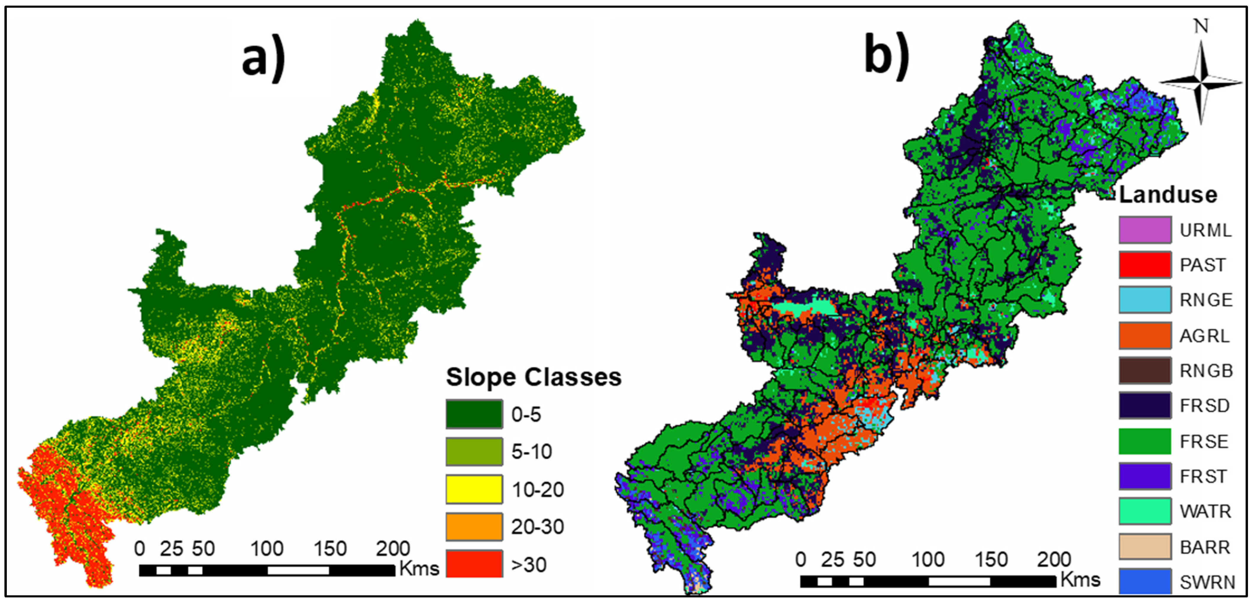
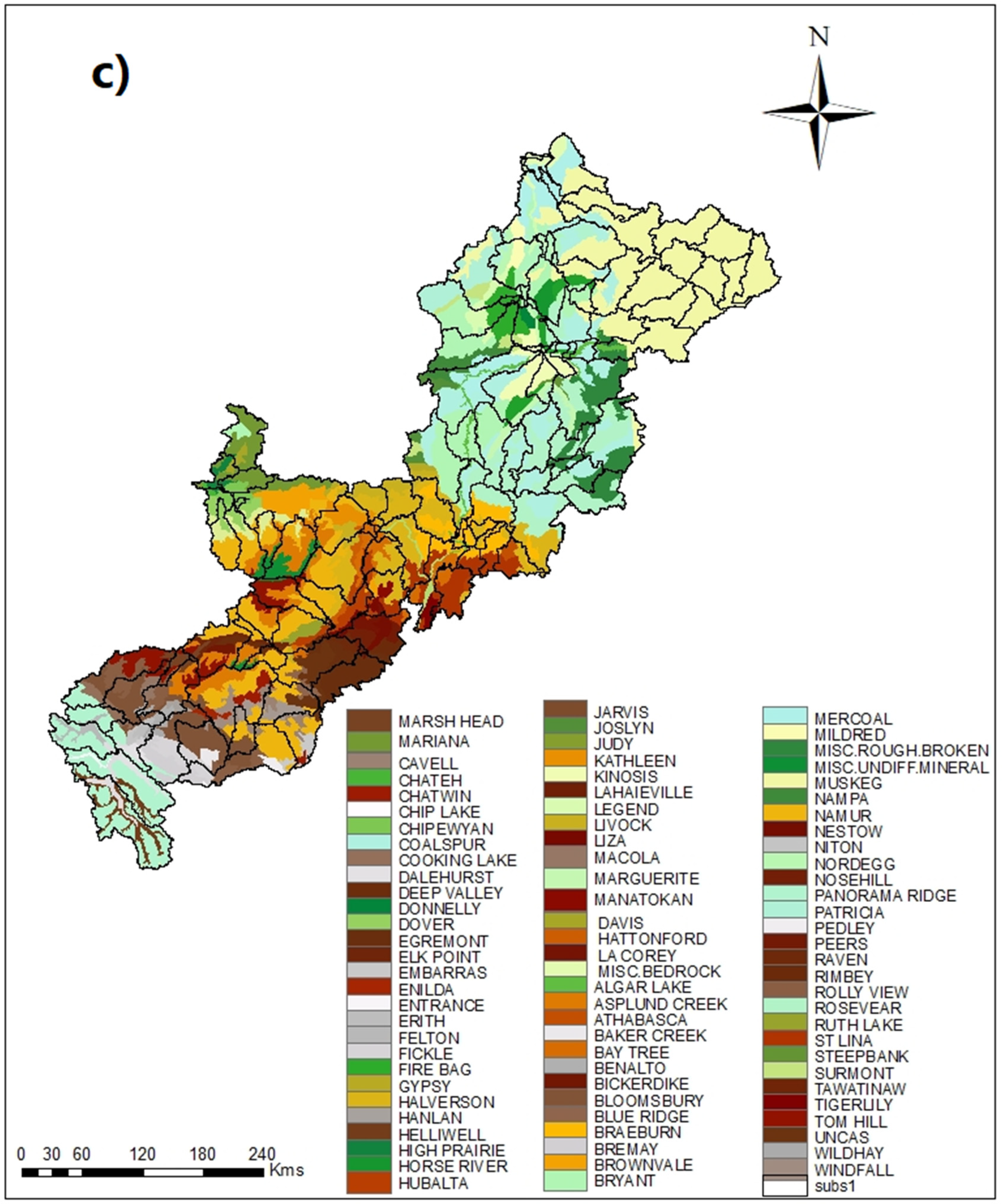
2.1. Study Area

This modeling research was carried out in the Athabasca River Basin, in the province of Alberta, Canada from 2006–2009 (Figure 1). The Athabasca River Basin, with an area of about 160, 935 km², drains to Lake Athabasca in northeastern Alberta, reaching towards the Arctic Ocean (Figure 1). Based on land-use cover mapping, about 80% of the Athabasca River Basin is covered with forest and about 10% of the basin is agricultural land. The climate of the area is categorized as subhumid, which is classified as short, cool summers and long, cold winters [19]. The mean annual air temperature was 1.1 °C and the mean annual precipitation was 461.07 mm.

2.2. Wetland Classification

In the Canadian wetland classification system, five wetland classes can be identified in terms of their characteristics and their presence in the Athabasca River Basin. The fens and bogs are the main dominant wetland classes in the Athabasca River Basin, where there are about 56% of bogs and about 17% of fen in the peat-covered wetlands with a higher water table (Figure 2). The rest (27%) of the basin is classified as swamps, open water bodies, and mixed wetland types.

2.3. Carbon Dioxide Emission Model from Wetlands

This study was performed by considering the significant effect of soil temperature, the groundwater table, and ecosystem respiration on CO₂ emissions at the watershed scale in the wetlands. The CO₂ emission model from peat decomposition was modified based on the interaction between the soil temperatures, groundwater table, and ecosystem respiration in CO₂ emission. The SWAT model permitted estimating these parameters in this research using the new SWAT model subroutine. The carbon cycle in the SWAT model included CO₂ emission, plant growth, litter decomposition (aerobic and anaerobic), and the below-ground carbon cycle (Figure 3).

The balance of carbon in the wetlands, A, was calculated based on the following equation [37]:

$$\mathrm{A}={\mathrm{P}}_{\mathrm{G}}-\left({\mathrm{R}}_{\mathrm{s}}+\mathrm{D}+\mathrm{W}+\mathrm{F}\right)$$

(1)

where PG is CO₂ uptake (µmol CO₂ m⁻² day⁻¹), ${\mathrm{R}}_{\mathrm{s}}$ is respiration (µmol CO₂ m⁻² day⁻¹), D is CO₂ from decomposition (µmol CO₂ m⁻² day⁻¹), W is weathering, and F is carbon loss via fire. Carbon emission to the atmosphere is marked negative, whereas CO₂ uptake is marked positive. The following equation represents the relationship between NEE and net ecosystem production (NEP):

$$\mathrm{NEE}=-\mathrm{NEP}$$

(2)

$$\mathrm{NEP}={ \mathrm{P}}_{\mathrm{G}}-{\mathrm{R}}_{\mathrm{s}}$$

(3)

$$\mathrm{NEP}=\mathrm{GPP}-\mathrm{RECO}$$

(4)

$$\mathrm{NEE}=\left(\left({\mathrm{GP}}_{\max }\times \mathsf{\alpha }\ast \mathrm{PPFD}\right)\times \left(\left(\mathsf{\alpha }\times \mathrm{PPFD}\right)+{ \mathrm{GP}}_{\max }\right){)}^{-1}\right)-\mathrm{RECO}$$

(5)

where NEE is the net ecosystem exchange (µmol CO₂ –C m⁻² day⁻¹), NEP is the net ecosystem production (µmol CO₂ –C m⁻² day⁻¹), PPFD is photosynthetic photon flux (µmol m⁻² day⁻¹), and α is the slope of the curve. Plant biomass (kg), GPP, and soil temperature (°C) are calculated by submodels of plant growth in the SWAT. RECO is the ecosystem respiration (µmol CO₂ m⁻² –C day⁻¹), which was calculated based on regressions between respiration rates and temperature using the Lloyd and Taylor equation [38]:

$$\mathrm{RECO}={ \mathrm{R}}_{\mathrm{ref}}{\mathrm{e}}^{{\mathrm{E}}_{\mathrm{o}}\left[\left(\frac{1}{{\mathrm{T}}_{\mathrm{ref}}-{\mathrm{T}}_0 }\right)-\left(\frac{1}{{\mathrm{T}}_{\mathrm{soil}}-{\mathrm{T}}_0}\right)\right]}+{\mathrm{R}}_{\mathrm{i}}$$

(6)

where E_o is the activation energy (K), T₀ (227.13 K) is the constant parameter, T_ref is the reference temperature (283.15), and Rh_i is the heterotrophic respiration (µmol CO₂ m⁻² day⁻¹) [38].

In the SWAT model, the daily average soil temperature was estimated based on the surface and the center of each soil layer. Soil layer temperature is a function of average annual temperature, surface temperature, and the depth of soil. Soil temperature for each layer was calculated within the SWAT models. For each hydrologic response unit, the soil temperature (T_soil) at the center of the soil layer (z) was calculated using the below equation [23]:

$${\mathrm{T}}_{\mathrm{soil}}\left(\mathrm{z}\right)={\mathsf{\gamma }\mathrm{T}{}^{\prime }}_{\mathrm{soil}}\left(\mathrm{z}\right)+\left(1-\mathsf{\gamma }\right)\times \left[\mathrm{d}\left({\mathrm{T}}_{\mathrm{Aair}}-{\mathrm{T}}_{\mathrm{sur}}\right)+{\mathrm{T}}_{\mathrm{sur}}\right]$$

(7)

where ${\mathrm{T}}_{\mathrm{soil}}$ is the soil temperature (°C), $\mathsf{\gamma }$ is the lag coefficient, $\mathrm{T}{{}^{\prime }}_{\mathrm{soil}}$ is the soil temperature (°C) at the depth (z), d is the depth (m), f is the actor, ${\mathrm{T}}_{\mathrm{Aair}}$ is the air temperature (°C) on the day, and ${\mathrm{T}}_{\mathrm{sur}}$ is the soil surface temperature (°C). The lag coefficient ($\mathsf{\gamma }$) is 0.8 for the SWAT. In our model, we used the Dual Arrhenius and Michaelis–Menten (DAMM) model equation to simulate soil respiration processes [39]:

$${\mathrm{Rh}}_{\mathrm{i}}={\mathrm{Rh}}_{0,\mathrm{i}}\times { \mathrm{C}}_{\mathrm{i}}\times \mathrm{f}\left({\mathrm{T}}_{\mathrm{soil}}\right)\times \Delta \mathrm{t}$$

(8)

$$\mathrm{f}\left(\mathrm{T}\right)=0.5\times \exp .\left({\mathsf{\beta }}_{\mathrm{i}}\times {\mathrm{T}}_{\mathrm{soil}}\right)$$

(9)

$${\mathrm{Rh}}_{\mathrm{i}}={\mathrm{Vmax}}_{\mathrm{i}}\times {\mathrm{C}}_{\mathrm{i}}\times {\mathrm{Enz}}_{\mathrm{av}}/\left({\mathrm{Km}}_{\mathrm{enz}}+{\mathrm{Enz}}_{\mathrm{av}}\right)\times {\mathrm{O}}_2/\left({\mathrm{Km}}_{\mathrm{O}2}+{\mathrm{O}}_2\right)$$

(10)

where Rh is the root trenching for heterotrophic respiration (µmol CO₂ C m⁻² day⁻¹), Rh₀ is the base rate, β_i is the parameter that varies among carbon pools, t is time, Vmax is the maximum velocity of reaction (day⁻¹), Km is the Michaelis–Menten half-saturation constant (µmol C m⁻³), Ci represents the SOM pool (µmol C m⁻²), T_soil is the soil temperature (°C), Enz_av is the active enzyme concentration for the reaction (µmol C m⁻³) and f is the function of the Michaelis–Menten (M–M) equation.

2.4. Description of the Model

A process-based, semi-distributed modified SWAT watershed model is applied to evaluate different processes in catchments, such as hydrology, sediment, and agricultural chemicals in different soil types, topography, land-cover, and land-use systems [18,21]. In our study, we modified the SWAT subroutine to evaluate its ability to predict CO₂ emissions by coupling groundwater, soil respiration, and soil temperature. The subroutines to predict CO₂ emission were at the hydrologic response unit (HRU) level. All the parameters, such as the biomass, soil temperature, groundwater table, and soil moisture, were calculated using the original SWAT and exchanged with the submodel of wetlands through Equations (1)–(10). Then the SWAT model was extended and deployed to the regional scale in estimating CO₂ emission, the groundwater table, soil temperature, net ecosystem exchange (NEE), and RECO observations in the cold wetlands of Alberta, Canada.

2.5. Model Inputs, Calibration, and Validation

A DEM, land-use map, and soil map were the basic inputs to set up the SWAT model for the Athabasca Basin [19,27] (Figure 4). A 90 m × 90 m digital elevation model (DEM), a 1 km × 1 km land-use map, and a 1:1 million-scale soil map [27] were used to build up the SWAT model of the Athabasca River Basin (

Table 1. SWAT land-use classification [18].

SWAT Land-Use Code	Land Use	Details
21	URML	Urban Medium Density
81	PAST	Pasture/Hay
71	RNGE	Grasslands/Herbaceous
85	AGRL	Generic
51	RNGB	Range Shrubland
41	FRSD	Deciduous Forest
42	FRSE	Evergreen Forest
43	FRST	Mixed Forest
11	WATR	Water
31	BARR	Bare Rock
33	SWRN	Southwestern Range

). Daily precipitation, maximum and minimum temperatures [27,40], relative humidity, solar radiation, and wind speed [41] were fed into the model. The watershed elevation was estimated at 207 m in the lower part of the Athabasca River Basin, whereas it is about 3669 m high in the mountainous part of the Athabasca River Basin (Figure 4). The soil input map was prepared and defined for the SWAT model. Climate data such as daily precipitation, maximum temperature, minimum temperature, relative humidity, and wind speed were used for the modified model input.

The monitoring site located in the Athabasca River Basin was used to obtain the groundwater table, RECO, CO₂, and NEE at the Fluxnet Canada Research Network (https://daac.ornl.gov/cgi-bin/dsviewer.pl?ds_id=1335; accessed on 31 January 2019). The data were obtained from the Flux Canada Research Network (FCRN), which is an easily accessible database on the Ameriflux website (https://ameriflux.lbl.gov/data/download-data/; accessed on 31 January 2019) with the necessary data policy (https://ameriflux.lbl.gov/data/data-policy/; accessed on 31 January 2019).

The SWAT-CU was used for the model calibration, validation, and uncertainty analysis [42,43]. The observed groundwater table, RECO, CO₂, and NEE data from 2006–2007 were used for calibration, and data from 2008–2009 were used for the validation processes. SWAT-CUP Sequential Uncertainty Fitting Version 2 (SUFI-2) was used for the sensitivity analysis [44]. The streamflow and the sediment load have been calibrated and validated, since sediment directly affects the transport amount of particular carbon and nitrogen. Because they are from the same river basin, the model coefficients related to streamflow and sediment transport can be used directly for the current study. Readers can refer to references for streamflow for the period (1983–2013) [27] and erosion and sediment transport for the period (1990–2006) [45]. Although the SWAT offers a wide range of parameters for sensitive analysis, we selected a limited number of parameters (

Table 2. SWAT model parameter calibration and sensitivity analysis for the Athabasca River Basin.

Parameter	SWAT Input File	Descriptions	Fitted Value	Min. Value	Max. Value	Rank
r__CN2	.mgt	SCS runoff curve number for moisture	0.16	−20	20	18
v__BIOMIX	.mgt	Biological mixing efficiency	0.76	0	1	19
v__CO2	.sub	Carbon dioxide concentration	285	0	800	4
r_CF	.hru	Decomposition response to soil temperature and moisture	0.07	0.5	1	13
r_CFDEC	.hru	Undisturbed soil turnover rate under optimum soil water and temperature	0.052	0.045	0.065	11
v__SOL_Z	.sol	Depth from soil surface to bottom of layer	145	0	3500	5
r_RSDCO	.bsn	Residue decomposition coefficient	0.06	0.02	0.1	14
v_SOL_CBN	.sol	Organic carbon content	2.7	0.05	10	15
v___R8	.gw	Lag coefficient for soil temperature	0.77	0	0.95	7
v__SOL_K	.sol	Soil hydraulic conductivity (mm/h)	0.45	0	5	17
v__SUB_SFTMP	.sno	Snowfall temperature (°C)	0.73	−7	7	6
v__SUB_SMTMP	.sno	Snowfall melt base temperature (°C)	2.1	−10	10	1
v__SUB_SMTMX	.sno	Maximum melt rate for snow during the year (mm/°C-day)	0.72	0	7.15	2
v__SUB_SMFMN	.sno	Minimum melt rate for snow during the year (mm/°C-day)	0.25	0	10	3
v__SUB_TIMP	.sno	Snowpack temperature lag factor	0.21	0.2	1	8
v__SOL_AWC	.sol	Soil available water storage capacity (mm H2O/mm soil)	0.35	0.2	0.4	12
v__SOL_ALB	.sol	Moist soil albedo	0.05	0	0.25	16
v__ESCO	.hru	Soil evaporation compensation factor	0.09	0	1	10
v__SNO50COV	.bsn	Snow water equivalent that corresponds to 50% snow cover	0.65	0	1	9

) that are known to influence the snowmelt, soil temperature, and carbon cycle in the studied river basin. The program generated different parameter sets from the specified range of values using the Latin hypercube (LH) sampling technique, which were regressed against the selected objective function. To identify the total predictive uncertainty band of the simulated results, the SWAT-CUP was run several times, each one identifying a narrower parameter range for each parameter (Table 1), until reasonable goodness-of-fit statistic values were achieved.

2.6. SWAT Model Statistical Evaluation

We used four metrics for statistical model evaluation to compare the measured and predicted CO₂ emissions. The R², NSE, RMSE, and the PBIAS were used to determine SWAT model performance [45].

$${\mathrm{R}}^2={\left[\frac{{{\displaystyle \sum }}_{\mathrm{i}=1}^{\mathrm{n}}\left({\mathrm{O}}_{\mathrm{i}}-\mathrm{Ō}\right)\left({\mathrm{E}}_{\mathrm{i}}-\mathrm{Ē}\right)}{\sqrt{{{\displaystyle \sum }}_{\mathrm{i}=1}^{\mathrm{n}}{\left({\mathrm{O}}_{\mathrm{i}}-\mathrm{Ō}\right)}^2}\sqrt{{{\displaystyle \sum }}_{\mathrm{i}=1}^{\mathrm{n}}{\left({\mathrm{E}}_{\mathrm{i}}-\mathrm{Ē}\right)}^2}}\right]}^2$$

(11)

where n is the number of observations, O_i is observed value, E_i is estimated value, Ō is the mean of observed values, Ē is the mean of estimated values, and i is the counter for individual observed and predicted values. R² values range between 0 and 1, where 1 indicates that the predicted value is equal to the observed value and 0 means that there is no correlation between the predicted and observed values.

$$\mathrm{NSE}=1-\frac{{{\displaystyle \sum }}_{\mathrm{i}=1}^{\mathrm{n}}{\left({\mathrm{E}}_{\mathrm{i}}-{\mathrm{O}}_{\mathrm{i}}\right)}^2}{{{\displaystyle \sum }}_{\mathrm{i}=1}^{\mathrm{n}}{\left({\mathrm{O}}_{\mathrm{i}}-\mathrm{Ō}\right)}^2}$$

(12)

The range of NSE lies between −∞ and 1.0 with NSE = 1 describing a perfect fit. Values 0 to 1.0 are generally viewed as acceptable levels of performance (the closer to 1.0, the better the model), whereas values <0 indicate that the mean observed value is a better predictor than the model. For biophysical (hydrological) models, NSE > 0.5 is generally considered good [46].

$$\mathrm{RMSE}=\sqrt{{\displaystyle \sum }_{\mathrm{i}=1}^{\mathrm{n}}\frac{{\left({\mathrm{O}}_{\mathrm{i}}-{\mathrm{E}}_{\mathrm{i}}\right)}^2}{\mathrm{n}}}$$

(13)

where RMSE is the root mean square error, O_i is the measured datum, E_i is the estimated value, Õ is the mean of the observed values, Ē is the mean estimated values, and n is the number of observations.

$$\mathrm{PBIAS}=\frac{{{\displaystyle \sum }}_{\mathrm{i}=1}^{\mathrm{n}}{\mathrm{O}}_{\mathrm{i}}-{\mathrm{E}}_{\mathrm{i}}}{{{\displaystyle \sum }}_{\mathrm{i}=1}^{\mathrm{n}}{\mathrm{O}}_{\mathrm{i}}}\times 100$$

(14)

where PBIAS is the percent bias, O_i is the measured datum, E_i is the estimated value, Õ is the mean of the observed values, Ē is the mean of estimated values, and n is the number of observations. The optimal value of PBIAS is 0, with low-magnitude values indicating accurate model simulation [46].

3. Results

3.1. Model Sensitivity

Sensitivity analysis was performed to identify the key sensitive parameters for calibration and validation processes in the SWAT model. The SWAT model has a wide range of parameters to perform sensitivity analysis. However, we selected the most sensitive and limited parameters for model calibration which influence CO₂ emission, including the groundwater table, soil temperature, and net ecosystem exchange (Table 1). Since the studied basin lies in a cold climate region, parameters related to snowmelt processes (SMTMP, TIMP, and SMFMN) were found to be sensitive. The parameter, v__SOL_Z (depth from the soil surface to the bottom of the layer), is the most sensitive in the cold wetland due to permafrost and the freeze-thaw cycle [20]. These parameters control the soil moisture dynamics. The validating model needs to accurately represent the snow-related process in such a cold climate watershed region. This is indeed expected in such a cold watershed region because snowmelt is the dominant hydrological process in the spring season. As the soil moisture has significant effects on CO₂ emission parameters, the soil moisture dynamics, such as SOL_AWC (available water storage capacity) and SOL_K (hydraulic conductivity), were also found to be quite sensitive as well. Three parameters related parameters with sensitive ranking (e.g., r_CN2, v_CO2, and v_SOL_CBN) were the most sensitive since they represent organic carbon and gas concentration. These parameter ranges and optimized values are given in Table 1.

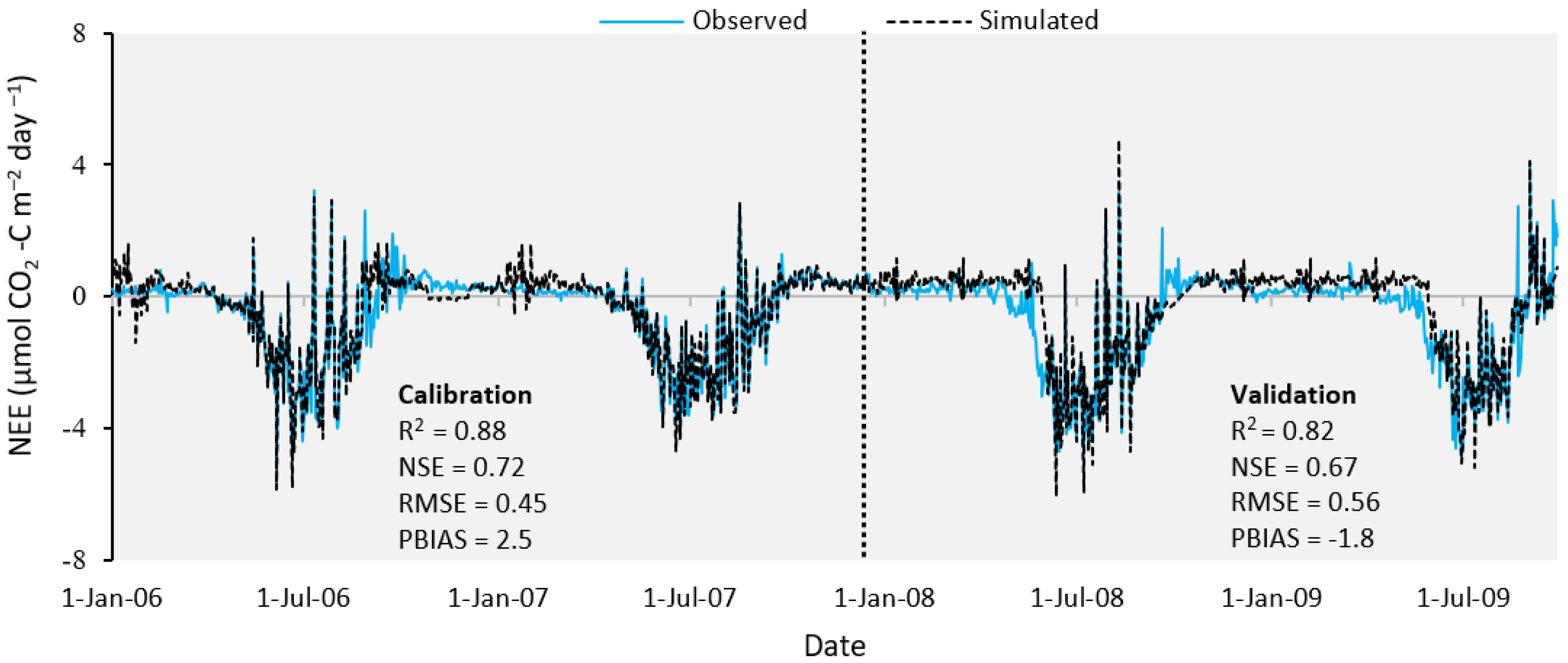
3.2. Net Ecosystem Exchange (NEE)

The simulated daily NEE indicated that the modified SWAT model could capture the variation of the daily observed NEE at the Athabasca River Basin during calibration and validation (Figure 5). The daily NEE was estimated very well in the calibration period with 0.88 for the value of R², and 0.82 for the validation period. The modified SWAT module indicated reasonably good results of NSE, RMSE, and PBIAS of 0.72, 0.45, and 2.5, respectively, for the calibration results. On the other hand, during the validation period, the model results also showed better model performance values of 0.67, 0.56, and −1.8, respectively (Figure 5). The comparison between the observed NEE and the simulated NEE values indicated a similar trend of increasing and decreasing values throughout the simulation period (Figure 5). The observed and simulated results confirmed that the SWAT model has a robust capacity to predict the NEE in the Athabasca watershed.

3.3. Groundwater Table

Groundwater table results showed fluctuation from season to season during 2006–2009. The observed groundwater table was within a range of 0.3–0.4 m from November to April, increasing to 0.5–0.8 m below the surface from May to August (Figure 6). It can be found that the model performed successfully in estimating the groundwater table. The model’s statistical efficiency gave very good results (R² = 0.85, NSE = 0.79) in the calibration (2006–2007) period. The SWAT model efficiency was also higher during the validation period, resulting in an R² of 0.81 and NSE of 0.72 in the Athabasca River Basin. The simulation results also showed a good model fit both during calibration and validation, giving RMSE and PBIAS values of 4.2 and 3.6 during calibration (2006–2007) and 5.2 and 5.3 during validation (2008–2009) periods, respectively.

3.4. Ecosystem Respiration

The highest ecosystem respiration (RECO) was estimated between June to September during calibration and validation. The lowest was observed between November and December (Figure 7). The RECO reached the maximum value in August, whereas lower values were observed in September. The trends of observed and simulated values depicted that the model has a better capability in predicting the values. The SWAT model performed very well in predicting ecosystem respiration with an R² of 0.81 for the calibration period and an NSE of 0.74 (Figure 7). However, the model efficiency during the validation period gave slightly lower results with an R² of 0.75 and NSE of 0.69 in the calibration period (Figure 7). The modified model slightly overpredicted RECO during the calibration and the validation period (Figure 7).

3.5. Soil Temperature

The observed daily soil temperature was used for a comparison with the simulation results in both calibration and validation periods. The estimated soil temperature results were in agreement with the observed ones in both the calibration and validation periods. It can be seen that the values of the corresponding metrics of R², NSE, PBIAS, and RMSE were 0.79, 0.74, −2.1, and 2.6, respectively, during the calibration period. The simulation result in the validation period also confirmed good results of R², NSE, RMSE, and PBIAS values being 0.76, 0.71, 3.2, and −2.6, respectively (Figure 8). This demonstrated that the simulated soil temperature was very well correlated with the observed soil temperature.

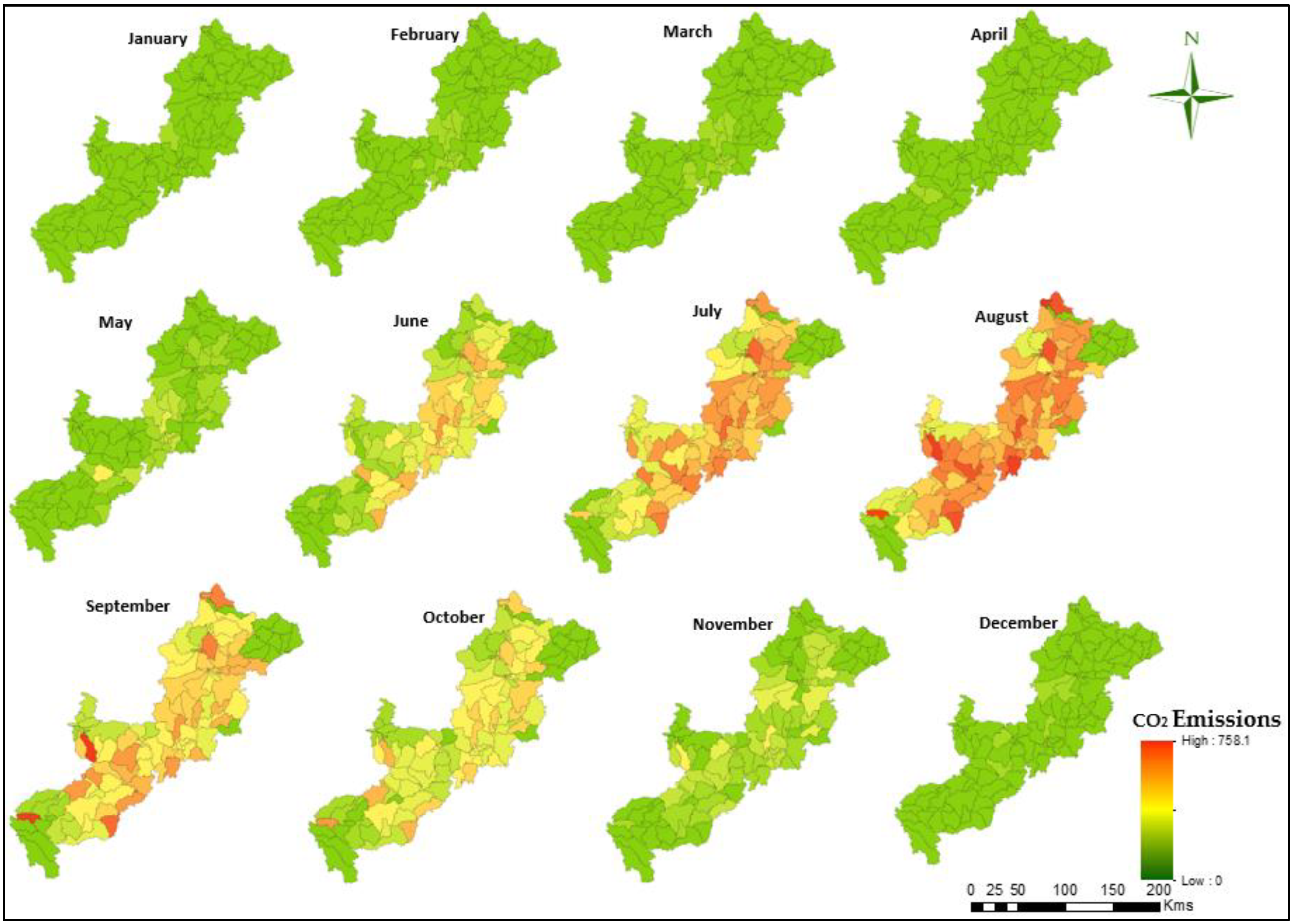
3.6. Carbon Dioxide Emission

The estimated CO₂ emission was predicted very well against the daily observed CO₂ emission, with R², NSE, RMSE, and PBIAS values of 0.71, 0.67, 3.2, and 2.6, respectively, in the calibration period (Figure 9). This showed that the predicted CO₂ emission results were well correlated with the observed CO₂ emission. Predicted CO₂ emission captured well the variation of the observed CO₂ emission in the calibration period (Figure 9). The model results gave an R² of 0.88 during the calibration and 0.85 during the validation period. Figure 10 shows a good model fit and correlation of the observed and predicted CO₂ and NEE during 2006–2009. This shows the modified SWAT model was suitable to estimate the CO₂ emissions and NEE.

3.7. Spatiotemporal Distribution of Carbon Dioxide Emissions

The spatiotemporal distribution of CO₂ emission was mapped in the Athabasca River Basin (Figure 11). The result reveals there is a significant variation in CO₂ emission both in space and time. The distribution of CO₂ emissions varies from month to month within the watershed. The emission trend shows an increase from January to July and a decrease of CO₂ emission from July to January in the study area. The maximum CO₂ was recorded in July, whereas the minimum emission was observed in June (Figure 11).

3.8. The Relationship between NEE, RECO, Soil Temperature, and CO₂ Emissions

Soil temperature, net ecosystem exchange, soil respiration, and groundwater are important to explain the fluctuations of CO₂ emissions from the soil. Figure 5, Figure 6 and Figure 7 and Figure 9 showed the effects of soil temperature on NEE, ecosystem respiration, and CO₂ emissions in the study period of 2006–2009. During the mid-summer season, higher RECO from the soil to the atmosphere in response to increased microbial metabolism was observed, resulting in significant increases of CO₂ emissions (Figure 7). During the winter period lower soil temperature and soil respiration rates were recorded and the simulated results also showed a similar trend. The low soil temperature and soil respiration during the midwinter in the study period (2006–2009) corresponded with lower CO₂ emissions. The nonlinear relationship was represented in Equation (6) as an increasing trend in CO₂ emission during the mid-summer when the soil temperature is higher.

However, despite increases in CO₂ emissions and RECO, NEE decreased as soil temperatures increased. This can be explained by the increase in plant photosynthesis, which utilizes CO₂ in the atmosphere. Biomass growth due to photosynthesis was calculated by the plant growth submodel in the SWAT, leading to increasing GPP. Finally, NEE decreased as the soil temperature increased in Equations (4)–(5). The modified SWAT model captured dynamics of NEE, ecosystem respiration, soil temperature, and CO₂ emission in the study period of 2006–2009. The prediction results of the modified SWAT model agreed with the observed CO₂ emission in the study periods at the river basin (

Table 3. Summary statistics.

Parameters	SWAT Model Fit Results
	R2 Value		NSE Value		RMSE		PBIAS
	Cal	Val	Cal	Val	Cal	Val	Cal	Val
NEE	0.88	0.82	0.72	0.67	0.45	0.56	2.5	−1.8
GWT	0.85	0.81	0.79	0.72	4.2	5.2	3.6	5.3
CO2	0.76	0.73	0.67	0.57	2.6	3.1	3.2	9.3
RECO	0.81	0.75	0.74	0.69	1.2	2.3	−2.3	−2.7
Tsoil	0.79	0.76	0.74	0.71	2.6	3.2	−2.1	−2.6

Note: NEE—net ecosystem exchange (µmol CO₂ –C m⁻² day⁻¹); GWT—groundwater table (m); CO₂—carbon dioxide (µmol CO₂ –C m⁻² day⁻¹); RECO—ecosystem respiration (µmol CO₂ –C m–2 day⁻¹); T_soil—soil temperature (°C); Cal—calibration; Val—validation.

). The modified model demonstrated the capability of the model to illustrate the trends and the nonlinear relationship between soil temperature, ecosystem respiration, and CO₂ emission from the cold wetlands of the Athabasca watershed.

4. Discussions

4.1. Advantages of the Modified SWAT Model

The SWAT model has been widely used for evaluating hydrologic and other watershed parameters worldwide [21,29,44,46,47,48,49,50]. However, the SWAT has not been tested to model CO₂ emission in cold wetlands, which are impacted by soil respiration, soil temperature, and the groundwater table [20]. In this study, the wetland subroutine in the SWAT was developed to add the new functions of the SWAT model in predicting CO₂ emission, soil temperature, NEE, RECO, and the groundwater table. The modified model showed a very good agreement between the observed and simulated values at the Athabasca River Basin. The modified SWAT model captured well the dynamics and the trends of soil temperature, NEE, RECO, and CO₂ emission from the cold wetlands in Canada. The spatiotemporal distribution of CO₂ emission showed significant variation in CO₂ emission both in space and time.

Our results quantified distinct seasonal variation and trends of the groundwater table and CO₂ emissions during the study period. The analysis showed an increased trend in CO₂ emissions in the summer season when the soil temperature is higher. During the mid-summer season, higher respiration was observed in the model results, which in turn was significant in affecting CO₂ emission. Based on our results, a high CO₂ emission was observed when the groundwater level remained at a depth below 0.5 m. In contrast, a lower emission was observed when the groundwater table was shallow. This can be explained by the lower groundwater table resulting in higher CO₂ emissions. The groundwater tables can significantly affect greenhouse gas emissions. This is in agreement with those using other approaches [51]. Their results showed that maximum CO₂ emission was observed from June to August, whereas minimum emission was observed from January to March. Similar studies also confirmed that the groundwater table has a significant impact on the release of CO₂ into the atmosphere [52,53]. Bubier et al. [26] also found that lower water tables corresponded with higher CO₂ emissions. Similarly, it is found that ecosystem respiration increased with increasing soil temperature and with decreasing groundwater level.

Ecosystem respiration had a good correlation with soil temperature. Similar findings reported impacts of soil temperature change on CO₂ emission in wetlands [19,54,55]. The minimum CO₂ emission was recorded from December to March due to lower soil temperature. The soil respiration and emission started increasing from June to September as the soil temperature increased. Increases in soil temperature increased CO₂ emission [56]. This indicates that CO₂ is affected by soil temperature which raises soil respiration during summer seasons in the wetlands [19,57,58,59,60,61,62]. The modified SWAT model captured well the daily NEE, RECO, water table, soil temperature, and CO₂ with a very good model efficiency.

4.2. Implications to Wetland Remediation and Reclamation, Limitation, and Future Research

The areas of wetlands cover more than 50% of the landscape in the Athabasca Oil Sands Region (AOSR). The wetlands in this region have been changed significantly due to the extensive development of the oil sands and the associated human activities. These disturbed changes can result in ecohydrological feedbacks that can affect the subsurface flow, water table, soil moisture, NEE, biodiversity, and peat decomposition. Wetland creation, restoration, and enhancement are commonly used to offset lost wetland functions. Despite the ubiquity of perturbations in the AOSR, knowledge of their cumulative impacts on wetland hydrologic functioning remains incomplete. Only a few studies have addressed the potential long-term changes to the groundwater table, which is a balance of charge and discharge in watersheds in the AOSR [33]. As a result, a better understanding of spatiotemporal variability with coupled groundwater dynamics in the region is an important first step before properly characterizing the impacts of perturbations, such as the construction of open mines, well pads, and industrial and living facilities on the recharge–discharge function of wetlands and the updated mitigation policy in the AOSR [33,63,64].

The modified SWAT model can simulate recharge–discharge water dynamics and their effects on the biogeochemical cycling, such as CO₂ and NEE, particularly in the wetlands. Because we kept all the functions of hydrological processes in the original SWAT, the modified SWAT model can analyze not only wetlands lost or degradation at the site scale, but also wetland variability at the regional scale due to the land-use change of wetland regions resulting from the human disturbance in past and present regional profiles. These past and present profiles of the wetland landscape can be used to make decisions regarding the type and location of restorations. This implies that a cumulative impact in reclamation and remediation could be estimated quantitatively to identify the key hydrologic variables, chemical variables, and charge-discharge in the wetland region over time and improve restoration practice.

However, the modified SWAT model has limitations. First, the HRU in the SWAT limits the resolution of the different types of wetlands, although this spatial resolution could be improved if small HRUs are used. In an HRU, all the wetlands are considered a percentage of the landscape, but wetland shape and boundary would not be resolved. Therefore, the modified SWAT remains to be developed in distinguishing different types of wetlands, such as bog, fen, marsh, and disturbed wetlands in the future. Soil parameters are spatially volume-averaged. This means that only one type of wetland can be represented in an HRU. Second, the validation results are slightly poor compared to calibration in Table 3. This is because the weather conditions have not been captured fully. In the cold region, it is still challenging to simulate the freeze-thaw cycle and permafrost process. CO₂ and CH₄ emissions are sensitive to the freeze-thaw cycle and permafrost processes [20]. This implies that the wetlands in the cold region are vulnerable to climate change. Finally, a restorative practice using different reclamation techniques requires development to represent wetland construction and restore disturbed areas. Varying levels of anthropogenic disturbance and different reclamation techniques should also be represented to account for both the reclamation practices and specific wetlands in the AOSR [65,66].

5. Conclusions

In this study, a wetland subroutine within the SWAT has been developed to consider the relationship between soil temperatures, the groundwater table, and ecosystem respiration on CO₂ emission. The modified SWAT model coupled soil temperature and groundwater with CO₂ emission, NEE, and RECO. The model was applied for estimating the CO₂ emission, NEE, RECO, and the groundwater table in the Athabasca River Basin. The model performance was examined against the observed data of CO₂ emission, NEE, and RECO in this region. The simulated results agreed well with the observed data, with satisfying statistical metrics in simulating NEE, RECO, CO₂, soil temperature, and groundwater. The modified model added new functions to the existing SWAT besides hydrological process modeling, which enhances the modeling capability of wetland processes such as greenhouse gas emissions. Our results show negative NEE in the Athabasca River Basin. The wetlands have a great capacity to absorb CO₂ via photosynthesis by the surface vegetation. CO₂ absorbed by photosynthesis could be higher than decomposition and soil respiration rates when biomass production is higher than peat decomposition. This provides a new tool and capability to investigate the spatiotemporal dynamics of CO₂ emissions, NEE, soil respiration, soil temperature, and the groundwater table in wetlands and watersheds and improve the restoration practices.

References

1. Gorham, E. Northern wetlands: Role in the carbon cycle and probable responses to climatic warming. Ecol. Appl. 1991, 1, 182–195. [Google Scholar] [CrossRef] [PubMed]
2. Yu, Z. Holocene carbon flux histories of the world’s wetlands: Global carbon-cycle implications. Holocene 2011, 21, 761–774. [Google Scholar] [CrossRef]
3. Frolking, S.E.; Bubier, J.L.; Moore, T.R.; Ball, T.; Bellisario, L.M.; Bhardwaj, A.; Carrol, P.; Crill, P.M.; Lafleur, P.M.; McCaughey, J.H.; et al. Relationship between ecosystem productivity and photosynthetically active radiation for northern wetlands. Glob. Biogeochem. Cycles 1998, 12, 115–126. [Google Scholar] [CrossRef] [Green Version]
4. Syed, T.H.; Famiglietti, J.S.; Chen, J.; Rodell, M.; Seneviratne, S.I.; Viterbo, P.; Wilson, C.R. Total basin discharge for the Amazon and Mississippi river basins from GRACE and a land-atmosphere water balance. Geophys. Res. Lett. 2005, 32, L24404. [Google Scholar] [CrossRef] [Green Version]
5. Blodau, C.; Moore, T.R. Experimental response of wetland carbon dynamics to a water table fluctuation. Aquat. Sci. 2003, 65, 47–62. [Google Scholar] [CrossRef]
6. Humphreys, E.R.; Lafleur, P.M.; Flanagan, L.B.; Hedstrom, N.; Syed, K.H.; Glenn, A.J.; Granger, R. Summer carbon dioxide and water vapor fluxes across a range of northern wetlands. J. Geophys. Res. 2006, 111, G04011. [Google Scholar] [CrossRef]
7. Kelly, R.A.; Jakeman, A.J.; Barreteau, O.; Borsuk, M.E.; ElSawah, S.; Hamilton, S.H.; Henriksen, H.J.; Kuikka, S.; Maier, H.R.; Rizzoli, A.E.; et al. Selecting among five common modelling approaches for integrated environmental assessment and management. Environ. Model. Softw. 2013, 47, 159–181. [Google Scholar] [CrossRef]
8. Butterbach-Bahl, K.; Baggs, E.M.; Dannenmann, M.; Kiese, R.; Boltenstern, S.Z. Nitrous oxide emissions from soils: How well do we understand the processes and their controls? Philos. Trans. R. Soc. B 2013, 368, 20130122. [Google Scholar] [CrossRef]
9. Parton, W.J.; Hartman, M.; Ojima, D.; Schimel, D. DAYCENT and its land surface sub model: Description and testing. Glob. Planet. Change 1998, 19, 35–48. [Google Scholar] [CrossRef]
10. Ogle, S.M.; Parton, W.J.; Cheng, K.; Pan, G. Using the DayCent Ecosystem Model to Predict Methane Emissions from Wetland Rice Production in Support for Mitigation Efforts. In Proceedings of the American Geophysical Union, Fall Meeting, abstract id. GC14B-12. San Francisco, CA, USA, 15–19 December 2014. [Google Scholar]
11. Leffelaar, P.A. Dynamics of partial anaerobiosis, denitrification, and water in a soil aggregate. Soil Sci. 1988, 146, 427–444. [Google Scholar] [CrossRef] [Green Version]
12. Leffelaar, P.A.; Wessel, W.W. Denitrification in a homogeneous, closed system. Soil Sci. 1988, 146, 335–349. [Google Scholar] [CrossRef]
13. Li, C.; Frolking, S.; Crocker, G.J.; Grace, P.R.; Klír, J.; Korchens, M.; Poulton, P.R. Simulating trends in soil organic carbon in long-term experiments using the DNDC model. Geoderma 1997, 81, 45–60. [Google Scholar] [CrossRef]
14. Zhang, Y.; Li, C.; Trettin, C.C.; Li, H.; Sun, G. An integrated model of soil, hydrology, and vegetation for carbon dynamics in wetland ecosystems. Glob. Biogeochem. Cycles 2002, 16, 1–17. [Google Scholar] [CrossRef] [Green Version]
15. Metivier, K.A.; Pattey, E.; Grant, R.F. Using the ecosys mathematical model to simulate temporal variability of nitrous oxide emissions from a fertilized agricultural soil. Soil Biol. Biochem. 2009, 41, 2370–2386. [Google Scholar] [CrossRef]
16. Grant, R.F.; Mekonnen, Z.A.; Riley, W.J. Mathematical Modelling of Arctic Polygonal Tundra with Ecosys: 1. Microtopography Determines How Active Layer Depths Respond to Changes in Temperature and Precipitation. J. Geophys. Res. Biogeosci. 2017, 122, 3161–3173. [Google Scholar] [CrossRef]
17. Waddington, J.M.; Morris, P.J.; Kettridge, N.; Granath, G.; Thompson, D.K.; Moore, P.A. Hydrological feedbacks in northern wetlands. Ecohydrology 2015, 8, 113–127. [Google Scholar] [CrossRef]
18. Arnold, J.G.; Moriasi, D.N.; Gassman, P.W.; Abbaspour, K.C.; White, M.J.; Srinivasan, R.; Santhi, C.; van Harmel, R.D.; van Griensven, A.; van Liew, M.W.; et al. SWAT: Model use, calibration, and validation. Trans. ASABE 2012, 55, 1491–1508. [Google Scholar] [CrossRef]
19. Melaku, N.D.; Wang, J.; Meshesha, T.W. Improving hydrologic model to predict the effect of snowpack and soil temperature on carbon dioxide emission in the cold region wetlands. J. Hydrol. 2020, 587, 124939. [Google Scholar] [CrossRef]
20. Wang, J.; Shrestha, N.K.; Delavar, M.A.; Meshesha, T.W.; Bhanja, S.N. Modelling Watershed and River Basin Processes in Cold Climate Regions: A Review. Water 2021, 13, 518. [Google Scholar] [CrossRef]
21. Melaku, N.D.; Renschler, C.S.; Holzmann, H.; Strohmeier, S.; Bayu, W.; Zucca, C.; Ziadat, F.; Klik, A. Prediction of soil and water conservation structure impacts on runoff and erosion processes using SWAT model in the northern Ethiopian highlands. J. Soils Sediments 2018, 18, 1743–1755. [Google Scholar] [CrossRef] [Green Version]
22. Bhanja, S.N.; Wang, J.; Shrestha, N.K.; Zhang, X. Modeling microbial kinetics and thermodynamic processes for quantifying soil CO2 emission. Atmos. Environ. 2019, 209, 125–135. [Google Scholar] [CrossRef]
23. Neitsch, S.L.; Arnold, J.G.; Kiniry, J.R.; Williams, J.R. Soil and Water Assessment Tool Theoretical Documentation: 2011, Version 2009; Grassland, Soil and Water Research Laboratory, Agricultural Research Service and Black land Research Center, Texas Agricultural Experiment Station: Temple, TX, USA, 2011. [Google Scholar]
24. Freeman, C.; Ostle, N.; Kang, H. An enzymatic ‘latch’ on a global carbon store. Nature 2001, 409, 149. [Google Scholar] [CrossRef] [PubMed]
25. Van Seters, T.E.; Price, J.S. The impact of peat harvesting and natural regeneration on the water balance of an abandoned cut over bog, Quebec. Hydrol. Proc. 2001, 15, 233–248. [Google Scholar] [CrossRef]
26. Bubier, J.L.; Bhatia, G.; Moore, T.R.; Roulet, N.G.; Lafleur, P.M. Spatial and temporal variability in growing-season net ecosystem carbon dioxide exchange at a large wetland in Ontario, Canada. Ecosystems 2003, 6, 353–367. [Google Scholar]
27. Shrestha, N.K.; Du, X.; Wang, J. Assessing climate change impacts on freshwater resources of the Athabasca River Basin, Canada. Sci. Total Environ. 2017, 601, 425–440. [Google Scholar] [CrossRef]
28. Du, X.; Shrestha, N.K.; Wang, J. Assessing climate change impacts on stream temperature in the Athabasca River Basin using SWAT equilibrium temperature model and its potential impacts on stream ecosystem. Sci. Total Environ. 2019, 650, 1872–1881. [Google Scholar] [CrossRef]
29. Melaku, N.D.; Wang, J. A modified SWAT Module for estimating Groundwater table at Lethbridge and Barons, Alberta, Canada. J. Hydrol. 2019, 575, 420–431. [Google Scholar] [CrossRef]
30. Voigt, C.; Marushchak, M.E.; Lamprecht, R.E.; Jackowicz-Korczyński, M.; Lindgren, A.; Mastepanov, M.; Granlund, L.; Christensen, T.R.; Tahvanainen, T.; Martikainen, P.J.; et al. Increased nitrous oxide emissions from Arctic wetlands after permafrost thaw. Proc. Natl. Acad. Sci. USA 2017, 114, 6238–6243. [Google Scholar] [CrossRef] [Green Version]
31. Cui, G.; Wang, J. Improving the DNDC biogeochemistry model to simulate soil temperature and emissions of nitrous oxide and carbon dioxide in cold regions. Sci. Total Environ. 2019, 687, 61–70. [Google Scholar] [CrossRef]
32. Rooney, R.C.; Bayley, S.E.; Schindler, D.W. Oil sands mining and reclamation cause massive loss of peatland and stored carbon. Proc. Natl. Acad. Sci. USA 2012, 109, 4933–4937. [Google Scholar] [CrossRef] [Green Version]
33. Volik, O.; Elmes, M.; Petrone, R.; Kessel, E.; Green, A.; Cobbaert, D.; Price, J. Wetlands in the Athabasca Oil Sands Region: The nexus between wetland hydrological function and resource extraction. Environ. Rev. 2020, 28, 246–261. [Google Scholar] [CrossRef]
34. Winter, T.C.; Rosenberry, D.O.; LaBaugh, J.W. Where does the ground water in small watersheds come from? Groundwater 2003, 41, 989–1000. [Google Scholar] [CrossRef]
35. Devito, K.J.; Creed, I.F.; Fraser, C.J.D. Controls on runoff from a partially harvested aspen-forested headwater catchment, Boreal Plain, Canada. Hydrol. Process. 2005, 19, 3–25. [Google Scholar] [CrossRef]
36. Wells, C.M.; Price, J.S. The hydrogeologic connectivity of a low-flow saline-spring fen peatland within the Athabasca oil sands region, Canada. Hydrogeol. J. 2015, 23, 1799–1816. [Google Scholar] [CrossRef]
37. Alm, J.; Talanov, A.V.; Saarnio, S.; Silvola, J.; Ikkonen, E.; Aaltonen, H.; Nykänen, H.; Martikainen, P.J. Reconstruction of the carbon balance for microsites in a boreal oligotrophic pine fen, Finland. Oecologia 1997, 110, 423–431. [Google Scholar] [CrossRef] [PubMed]
38. Lloyd, J.; Taylor, J.A. On the temperature dependence of soil respiration. Funct. Ecol. 1994, 8, 315–323. [Google Scholar] [CrossRef]
39. Sihi, D.; Eric, A.; Davidson, E.A.; Chen, M.; Savage, K.E.; Richardson, A.D.; Keenan, T.F.; Hollinger, D.Y. Merging a mechanistic enzymatic model of soil heterotrophic respiration into an ecosystem model in two AmeriFlux sites of northeastern USA. Agric. For. Meteorol. 2018, 252, 155–166. [Google Scholar] [CrossRef] [Green Version]
40. GoC. Environment and Natural Resources: Weather, Climate and Hazard; GoC, Ed.; GoC: London, UK, 2016; Available online: http://climate.weather.gc.ca/ (accessed on 31 January 2019).
41. CFSR. Climate Forecast System Reanalysis. G.W.D.f.S (Global Weather Data for SWAT), Ed.; 2016. Available online: http://globalweather.tamu.edu (accessed on 31 January 2019).
42. Abbaspour, K.C.; Yang, J.; Maximov, I.; Siber, R.; Bogner, K.; Mieleitner, J.; Zobrist, J.; Srinivasan, R. Modelling hydrology and water quality in the pre-alpine/alpine Thur watershed using SWAT. J. Hydrol. 2007, 333, 413–430. [Google Scholar] [CrossRef]
43. Abbaspour, K.C.; Rouholahnejad, E.; Vaghefi, S.; Srinivasan, R.; Yang, H.; Kløve, B. A continental-scale hydrology and water quality model for Europe: Calibration and uncertainty of a high-resolution large-scale SWAT model. J. Hydrol. 2015, 524, 733–752. [Google Scholar] [CrossRef] [Green Version]
44. Abbaspour, K.C.; Johnson, C.A.; van Genuchten, M.T. Estimating uncertain flow and transport parameters using a sequential uncertainty fitting procedure. Vadose Zone J. 2004, 3, 1340–1352. [Google Scholar] [CrossRef]
45. Shrestha, N.K.; Wang, J. Predicting sediment yield and transport dynamics of a cold climate region watershed in changing climate. Sci. Total Environ. 2018, 625, 1030–1045. [Google Scholar] [CrossRef] [PubMed]
46. Moriasi, D.N.; Gitau, M.W.; Pai, N.; Daggupati, P. Hydrologic and water quality models: Performance measures and evaluation criteria. Trans. ASABE 2015, 58, 1763–1785. [Google Scholar]
47. Zhang, X.; Izaurralde, R.C.; Manowitz, D.H.; Sahajpal, R.; West, T.O.; Thomson, A.M.; Xu, M.; Zhao, K.; LeDuc, S.D.; Williams, J.R. Regional scale cropland carbon budgets: Evaluating a geospatial agricultural modeling system using inventory data. Environ. Model. Softw. 2015, 63, 199–216. [Google Scholar] [CrossRef] [Green Version]
48. Zhang, X.; Izaurralde, R.C.; Arnold, J.G.; Williams, J.R.; Srinivasan, R. Modifying the soil and water assessment tool to simulate cropland carbon flux: Model development and initial evaluation. Sci. Total Environ. 2013, 463–464, 810–822. [Google Scholar] [CrossRef] [PubMed]
49. Tan, M.L.; Gassman, P.W.; Srinivasan, R.; Arnold, J.G.; Yang, X. A Review of SWAT Studies in Southeast Asia: Applications, Challenges and Future Directions. Water 2019, 11, 914. [Google Scholar] [CrossRef] [Green Version]
50. Krysanova, V.; White, M. Advances in water resources assessment with SWAT—An overview. Hydrol. Sci. J. 2015, 60, 771–783. [Google Scholar] [CrossRef] [Green Version]
51. Leduc, S.D.; Zhang, X.; Clark, C.M.; Izaurralde, R.C. Cellulosic feedstock production on Conservation Reserve Program land: Potential yields and environmental effects. GCB Bioenergy 2016, 9, 460–468. [Google Scholar] [CrossRef]
52. Meshesha, T.W.; Wang, J.; Melaku, N.D. Modelling spatiotemporal patterns of water quality and its impacts on aquatic ecosystem in the cold climate region of Alberta, Canada. J. Hydrol. 2020, 587, 124952. [Google Scholar] [CrossRef]
53. Baah-Acheamfour, M.; Carlyle, C.N.; Lim, S.S.; Bork, E.W.; Chang, S.X. Forest and grassland cover types reduce net greenhouse gas emissions from agricultural soils. Sci. Total Environ. 2016, 571, 1115–1127. [Google Scholar] [CrossRef]
54. Oviedo-Vargas, D.; Genereux, D.P.; Dierick, D.; Oberbauer, S.F. The effect of regional groundwater on carbon dioxide and methane emissions from a lowland rainforest stream in Costa Rica. J. Geophys. Res. Biogeosci. 2015, 120, 2579–2595. [Google Scholar] [CrossRef]
55. Mishra, V.; Asoka, A.; Vatta, K.; Lall, U. Groundwater depletion and associated CO2 emissions in India. Earth’s Future 2018, 6, 1672–1681. [Google Scholar] [CrossRef]
56. Euskirchen, E.S.; Edgar, C.W.; Turetsky, M.R.; Waldrop, M.P.; Harden, J.W. Differential response of carbon fluxes to climate in three wetland ecosystems that vary in the presence and stability of permafrost. J. Geophys. Res. Biogeosci. 2014, 119, 1576–1595. [Google Scholar] [CrossRef]
57. Hassan, W.; Bano, R.; Khatak, B.U.; Hussain, I.; Yousaf, M.; David, J. Temperature sensitivity and soil organic carbon pools decomposition under different moisture regimes: Effect on total microbial and enzymatic activity. Clean Soil Air Water 2015, 43, 391–398. [Google Scholar] [CrossRef]
58. Moore, T.R.; Dalva, M. The influence of temperature and water table position on carbon dioxide and methane emissions from laboratory columns of wetland soils. J. Soil Sci. 1993, 44, 651–664. [Google Scholar] [CrossRef]
59. Gundersen, P.; Christiansen, J.R.; Frederiksen, P.; Vesterdal, L. Influence of hydromorphic soil conditions on greenhouse gas emissions and soil carbon stocks in a Danish temperate forest. For. Ecol. Manag. 2012, 284, 185–195. [Google Scholar]
60. Gritsch, C.; Zimmermann, M.; Zechmeister-Boltenstern, S. Interdependencies between temperature and moisture sensitivities of CO2 emissions in European land ecosystems. Biogeosciences 2015, 12, 5981–5993. [Google Scholar] [CrossRef] [Green Version]
61. Bhanja, S.N.; Wang, J. Influence of environmental factors on autotrophic, soil and ecosystem respirations in Canadian boreal forest. Ecol. Indic. 2021, 125, 107517. [Google Scholar] [CrossRef]
62. Bhanja, S.N.; Wang, J. Estimating influences of environmental drivers on soil heterotrophic respiration in the Athabasca River Basin, Canada. Environ. Pollut. 2020, 257, 113630. [Google Scholar] [CrossRef]
63. Susilawati, L.H.; Setyanto, P.; Ariani, M.; Hervani, A.; Inubushi, K. Influence of water depth and soil amelioration on greenhouse gas emissions from peat soil columns. Soil Sci. Plant Nutr. 2016, 62, 57–68. [Google Scholar] [CrossRef] [Green Version]
64. Government of Alberta. Alberta Wetland Restoration Directive. Environment & Sustainable Resource Development, 2016 Water Policy Branch; Alberta Environment and Parks: Edmonton, AB, Canada, 2016. [Google Scholar]
65. Hwang, H.T.; Park, Y.J.; Sudicky, E.A.; Berg, S.J.; McLaughlin, R.; Jones, J.P. Understanding the water balance paradox in the Athabasca River Basin, Canada. Hydrol. Process. 2018, 32, 729–746. [Google Scholar] [CrossRef]
66. Amponsah, N.Y.; Wang, J.; Zhao, L. A review of life cycle greenhouse gas (GHG) emissions of commonly used ex-situ soil treatment technologies. J. Clean. Prod. 2018, 186, 514–525. [Google Scholar] [CrossRef]
Figure 1. DEM map of Athabasca River Basin and location of flux station.
Water 14 01458 g001
Figure 2. Wetland distribution in the study’s river basin and Canada.
Water 14 01458 g002
Figure 3. Conceptual model of CO2 emission processes in the Wetlands.
Water 14 01458 g003
Figure 4. Model input: slope classification of Athabasca River Basin derived from DEM (a), and land-use/land-cover classification of Athabasca River Basin (b). Model input: soil maps of Athabasca River Basin (c).
Water 14 01458 g004aWater 14 01458 g004b
Figure 5. NEE calibration and validation results at Athabasca River Basin.
Water 14 01458 g005
Figure 6. Observed and simulated daily groundwater table for the calibration and validation periods.
Water 14 01458 g006
Figure 7. Predicted and observed daily RECO in the calibration and validation periods.
Water 14 01458 g007
Figure 8. Predicted and observed daily soil temperature in the calibration and validation periods.
Water 14 01458 g008
Figure 9. Predicted and observed daily CO2 emission in the calibration and validation periods.
Water 14 01458 g009
Figure 10. Observed and simulated daily NEE ((a) calibration, (b) validation)) and CO2 emission ((c) calibration, (d) validation).
Water 14 01458 g010
Figure 11. Spatiotemporal CO2 Emissions (µmol CO2–C m−2 day−1).
Water 14 01458 g011