Article

Improving Jakarta’s Katulampa Barrage Extreme Water Level Prediction Using Satellite-Based Long Short-Term Memory (LSTM) Neural Networks

by
Hadi Kardhana
1,
Jonathan Raditya Valerian
2,
Faizal Immaddudin Wira Rohmat
1,3,* and
Muhammad Syahril Badri Kusuma
1
1
Faculty of Civil and Environmental Engineering, Institut Teknologi Bandung, FTSL Building, Jalan Ganesa No. 10, Bandung 40132, West Java, Indonesia
2
Master Program of Water Resources Management, Faculty of Civil and Environmental Engineering, Institut Teknologi Bandung, MPSDA Building, Jalan Ganesa No. 10, Bandung 40132, West Java, Indonesia
3
Water Resources Development Center, Institut Teknologi Bandung, CIBE Building 5th Floor, Jalan Ganesa No. 10, Bandung 40132, West Java, Indonesia
*
Author to whom correspondence should be addressed.
Water 2022, 14(9), 1469; https://doi.org/10.3390/w14091469
Submission received: 19 March 2022 / Revised: 21 April 2022 / Accepted: 28 April 2022 / Published: 4 May 2022
(This article belongs to the Special Issue Numerical Simulations and Modelling of Extreme Flood Events)

Abstract

:
Jakarta, the capital region of Indonesia, is experiencing recurring floods, with the most extensive recording loss as high as 350 million dollars. Katulampa Barrage’s observation of the Upper Ciliwung River plays a central role in reducing the risk of flooding in Jakarta, especially flowing through the Ciliwung River. The peak flow measured in the barrage would travel 13–14 h to the heart of the city, providing adequate time for the government officials and the residents to prepare for the flood risk. However, Jakarta is continually pressed by the population growth, averaging 1.27% in the past 20 years. The constant growth of Jakarta’s population continually develops slums in increasingly inconvenient locations, including the riverbanks, increasing vulnerability to floods. This situation necessitates a more advanced early warning system that could provide a longer forecasting lead time. Satellite remote sensing data propose a promising utility to extend the prediction lead time of extreme events. In the case of this study, Sadewa data is used to predict the water level of Katulampa Barrage using long short-term memory (LSTM) recurrent neural networks (RNN). The results show that the model could predict Katulampa Water Level accurately. The model presents a potential for implementation and additional lead time to increase flood mitigation preparedness.

1. Introduction

Flooding is a natural hazard with far-reaching consequences in Indonesia, a tropical equatorial country with approximately 270 million people. In 2020 alone, 1065 flood events occurred across Indonesia, more than a third of the total combined 2925 disasters in the year, including floods, flash floods, landslides, hurricanes, droughts, forest and land fires, extreme tidal waves, earthquakes, and volcanic eruption [1]. Indonesia has a monsoon climate and has high annual rainfall and extreme flash rainfall. The Jakarta 2020 new-year flood that occurred during the dawn of 1 January 2020 was reported to have a 377 mm rainfall throughout 24 h period recorded on ground station apparatuses [2]. Prior studies stated that Jakarta is one of the most flood-prone cities globally. The 2007 flood cost the city 350 million dollars, of which 74% of the total loss occurred in residential areas. In 2013, Jakarta experienced another major flood in which 124 villages (kelurahan) were inundated with fatalities [3,4,5]. The first historical flood event recorded in the city was in 1619 during the Dutch colonial era; however, the frequency of flood events is increasingly becoming more frequent [6,7,8]. Prior studies attribute such change to the land-use change both in the highlands and lowlands of the area, land subsidence, sea-level rise, and the direct and indirect consequences of uncontrolled urbanization pressures [4,9,10].
Jakarta is continually pressed by the population growth, averaging 1.27% in the past 20 years [11]. As a result of the rising population, Jakarta’s peri-urban and rural areas are being converted into build zones to meet the growing demand for housing, commercial, and industrial operations [12,13]. Inside the Jakarta City border, the constant growth of Jakarta’s population continually develops slums as a consequence of poor spatial planning and lax law enforcement [14,15]. The slums develop in increasingly inconvenient locations, including the riverbanks, which increases the vulnerability to floods [10,16]. For flood event preparedness, the current method relies on the measured Katulampa Barrage water level observation. The observation of the barrage is communicated to the civil servants and the residents in the case of a potential flood. The peak flow observed at Katulampa Barrage would reach the heart of Jakarta City between 13–14 h [17] through the Ciliwung River (Figure 1). Such a limited lead time window of 13–14 h of forecast between Katulampa and the heart of Jakarta City has been adequate to minimize flood risk. However, the ever-increasing threat of the Jakarta flood and the increasing vulnerability necessitates a more advanced early warning system that could provide a longer forecasting lead time.
Satellite remote sensing data propose a promising utility to extend the prediction lead time of extreme events. Conventionally, a three-step process needs to be performed to produce water levels from satellite data. The usual process uses weather research and forecasting models (WRF) to predict rainfall from satellite data [18,19]. The rainfall data is then passed into a rainfall-runoff model to simulate the ground-level hydrological process. Some examples of the commonly used rainfall-runoff models are SAC-SMA [20] and NRECA [21]. Machine learning models, on the other hand, bypass the required step of having an intermediate rainfall and discharge data modeling. Instead, the model would act as a black box inputting satellite reading to learn to predict water level. In the case of this study, Sadewa data is used to predict the water level of Katulampa Barrage. Machine learning has gained substantial traction in academic and practical fields in the past decade due to its robustness in classification, pattern recognition, and prediction. In flood-related research, the application is widespread both in the dimension of data source and the application.
Table 1 compares some of the more recent publications related to the machine learning based-prediction model in flood-related research in relation to this research. The table maps different data sources, i.e., water level, discharge data, rainfall, meteorological data, radar, and satellite, to predict output variables, i.e., water level, discharge, or rainfall. The most straightforward implementation to predict future data is the previously occurred data of the same datatype, which in the case of the example studies presented in Table 1, are inside the shaded cells. An example is the prediction of the current discharge based on previous discharge records. Such a system provides auspicious performance of R2 values nearing one when predicting t + 1 data [22,23,24,25,26,27,28,29]. However, the performance would drop by 10–20% as the models predict t + 6 data [24,25,28,30]. Other studies utilize different datatype to produce early warning lead time, e.g., predicting rainfall using satellite data [31,32], predicting rainfall using radar data [33,34], predicting rain using meteorological data [35,36], predicting discharge using meteorological data [37], predicting discharge using rainfall [38,39,40], and predicting water level using rainfall [41,42].
Various studies cited in Table 1 suggest long short-term memory (LSTM) recurrent neural networks (RNN) is the “default-go-to approach” to solve timeseries hydrological problems, due to the faster ability to iterate more model configurations. This study aims to demonstrate Sadewa satellite dataset observation to predict water level at the Katulampa Barrage, i.e., the Sadewa satellite dataset acts as an input to the prediction of Katulampa Barrage water level. This study uses the application of LSTM-RNN as the prediction engine and presents the performance comparison to simple artificial neural networks (ANN) and RNN runs. The Sadewa dataset includes thirteen variables, including temperature, cloud growth, accumulated hourly rainfall, and other atmospheric and surface readings, with details presented in subsequent sections. The model development aims to extend the forecast lead-time to minimize the risk of flooding in Jakarta.

2. Materials and Methods

2.1. Ciliwung River Characteristics

Jakarta, the capital of Indonesia, experiences a tropical monsoon climate. Although generally having only a small amount of rain during the dry season, rainfall during the rainy season could sometimes pour heavily during a short time, e.g., more than 100 mm in only 2–6 h, due to its climate and topography. Jakarta is a naturally flood-prone area [9]. The oldest recorded data of flood events was in 1619 during the Dutch colonial era. Based on that, the colonial government developed a flood canal system to mitigate floods in Jakarta. In the recent period, due to the sheer damage caused by the 2007 flood event, updated mitigation plans were made using this 2007 flood as the reference [48]. The upper part of the Jakarta Region has undergone a rapid and uncontrolled land-use change [4], including the Ciliwung watershed, one of the most important of the thirteen watersheds flowing into the Jakarta Metropolitan Area.
Ciliwung’s main river length is 124 km, with headwaters starting from the Bogor Regency, where the location of Katulampa Barrage is marked as the limit of the Upper Ciliwung Watershed (Figure 1). The river flows through Bogor City and Depok City before entering the Jakarta City limit right after the Depok Gauge. The elevation of Ciliwung ranges from 0 to 2985 m. Ciliwung watershed area is 370 km2 with an average width of 3 km. The elongated and narrow shape is a typical watershed feature in the thirteen neighboring watersheds. The average annual precipitation in the basin is 3125 mm, while the average annual temperatures are 26.3 °C and 28.8 °C in the upstream and downstream areas, respectively [8,12]. The maximum and minimum temperature recorded was 34 °C and 19 °C, respectively [49]. Forest, dry agriculture, paddy fields, urban area, and water are the different land-use types in the watershed with a rapid rate of urbanization [50,51].
Initially, most Ciliwung watershed area, especially the Upper Ciliwung Catchment, was intended as a conservation area. Indicated by the maximum (Qmax) and minimum (Qmin) discharge ratio, the Ciliwung watershed was classified as a healthy river in 1977–1984 with Qmax/Qmin a value ratio of 14.4. However, the ratio deteriorated to 33.8 in 1985–1990, then 148.1 in 1990–1995, and further to 283.8 in 1996–2002 [52], indicating the river condition has worsened. Due to such rapid and uncontrolled urbanization, flood in the Jakarta region is increasingly frequent [9,48,52], increasing the average annual potential damage. Recent studies focused on understanding the rainfall-runoff process in the river basin with the aim of reducing the risk of flood damage further [48,53,54,55].

2.2. Ciliwung Flood Early Warning System

The current strategy for flood event preparedness relies on the measured Katulampa Barrage water level observation (Figure 2). According to general observation, the peak flow measured at Katulampa Barrage would reach the center of Jakarta City between 13–14 h through the Ciliwung River [17]. Such lead time gives a chance to the local governance to spread flood risk warning messages through the radio system. The flood risk information would first come from the gatekeeper at the barrage and several other flood gates. The gatekeeper would convey the information to the civil servants at the provincial and subdistrict (kecamatan) levels. The information is then conveyed to the village/kampong (kelurahan) leader, who is tasked with spreading the warning messages among the residents. In the case of extreme events, the gatekeeper could inform the kampong leaders directly to evacuate their residents. In such severe cases, the governance, in cooperation with the KORAMIL (the sub-district military command), is responsible for evacuation, flood damage mitigation, and rescue tasks [56].
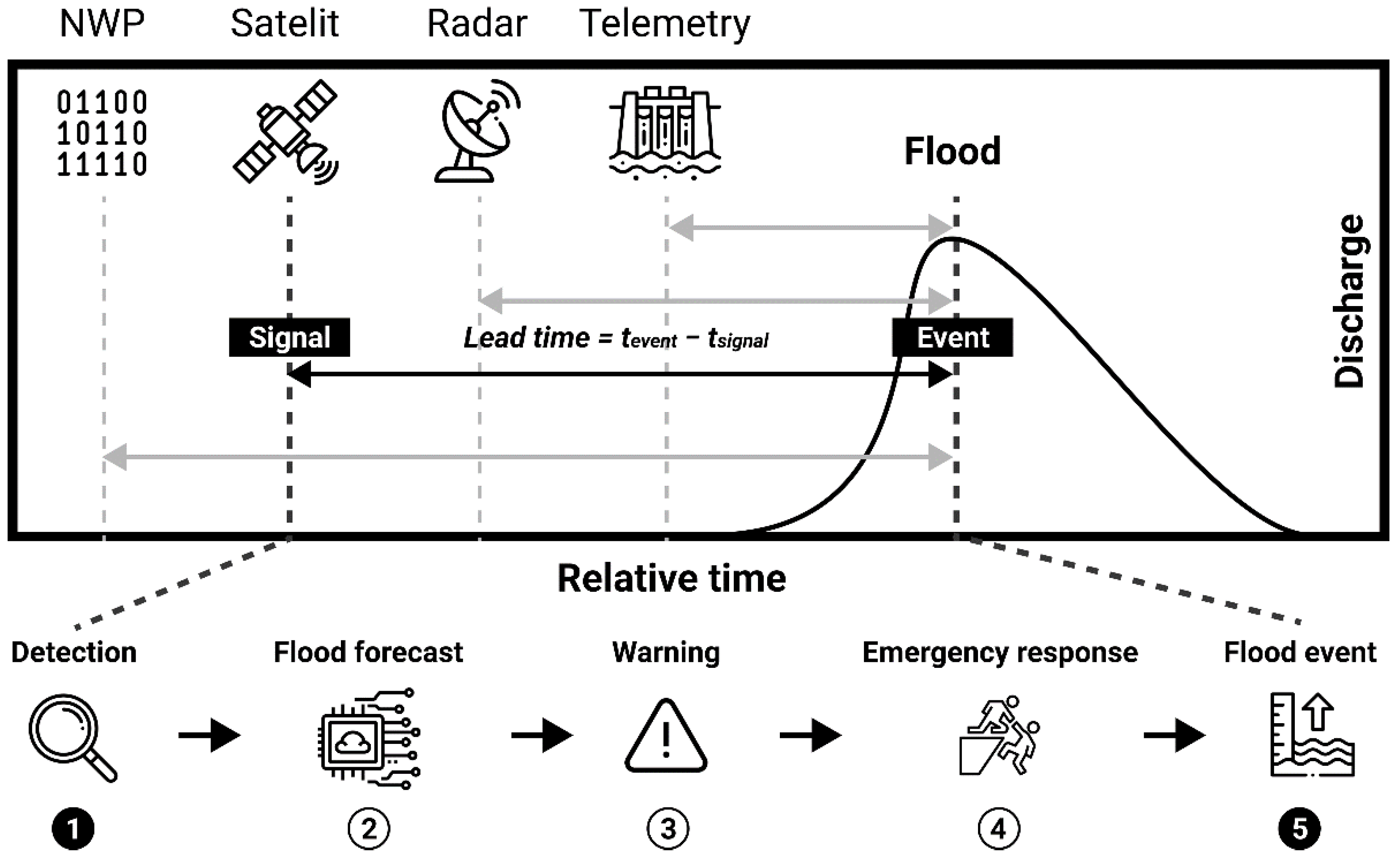
Although the region has adapted to the current lead time window, the ever-increasing risk of flooding in Jakarta necessitates the development of a more effective early warning system capable of providing an earlier forecasting lead time. Figure 2 illustrates the different data type usages to increase flood prediction lead time. The current Katulampa measurement through visual observation and telemetry provides a warning for flood events downstream—in this case, 13–14 h of lead time before the flood reaches the Manggarai area (Figure 1). Doppler-based radar readings on cloud formation and rainfall could provide a longer lead time while at the same time being relatively accurate. However, such an instrument is not currently available in the area, thus requiring significant investment. Satellite data can provide an early indication of ground events in atmospheric levels before reaching the land. Those early indications can be understood as longer lead-time compared to ground-based observation, e.g., water level measurement. An even longer lead time can be achieved by utilizing numerical weather predictions (NWPs); however, the discussion of such methods and their uncertainties is beyond the scope of this study.

2.3. Source Dataset

There are two types of data collected: satellite and water level data. The satellite data was collected from the Sadewa program (https://sadewa.sains.lapan.go.id, accessed on 19 January 2022), a research and development product developed by the Center for Atmospheric Science and Technology (PSTA)—National Institute of Aeronautics and Space (LAPAN), Indonesia [57]. Thirteen Sadewa inputs variables are used: (1) CCLD—composite observation showing growing cloud criteria; (2) B04—near-infrared observation channel; (3) IR1—peak cloud temperature observation channel; (4) IR3—water vapor observation channel; (5) VIS—visible observation channel; (6) cloud—predicted cloud fraction; (7) psf—predicted perturbation pressure; (8) qvapor—predicted total column water vapor (humidity levels); (9) rain—predicted accumulated rain per hour; (10) sst—predicted surface temperature; (11) wind—predicted wind speed and direction at an altitude of 1.458 m; (12) winu—predicted wind speed and direction at an altitude of 11.787 m; and (13) wn10—predicted near-surface wind speed and direction at 10 m [58]. Datasets collected from Sadewa consist of raster images of 1000 × 400 pixels spanning between 95° to 145° longitude and −10° to 10° latitude. Each pixel cell size is 0.05 × 0.05 decimal degrees in the horizontal and vertical directions, approximately 5.55 km × 5.55 km. Thus, each cell area coverage is approximately 30.8 km2.
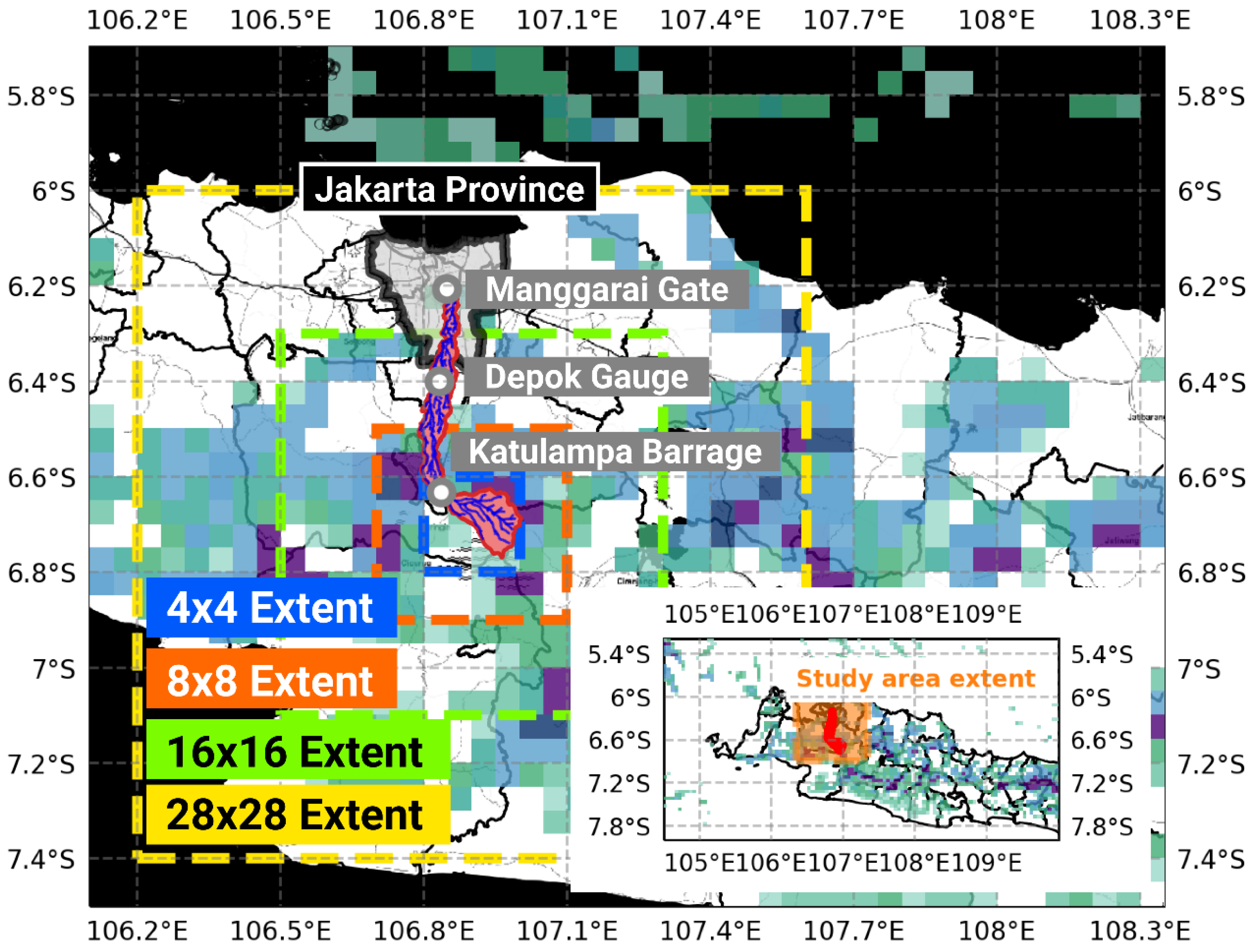
Water level data is sourced from the Jakarta Department of Water Resources (DWR) website (http://poskobanjirdsda.jakarta.go.id, accessed on 19 January 2022), managed by the Jakarta Department of Water Resource Data and Information Center. The website displays information on the status, water levels graph, and river water levels in Jakarta and provides notifications regarding the alert status of floodgates, providing real-time water level data across 21 water level measurement points with a temporal resolution of 10-min [59]. Although the water level data has been publicly available since 1 January 2013, the study is limited by the availability and hourly temporal resolution of Sadewa data. In terms of public availability, Sadewa data prior to 2019 is not publicly accessible. Hence, the dataset used in this study is an hourly dataset ranging from 1 January 2019, through 31 December 2020. Spatially, there are four extents of data in consideration. The summary of the source dataset used in this study is presented in Table 2. Figure 3 shows that the Katulampa Watershed is entirely inside the 4 × 4 Sadewa cell extents, one of the data clipping extents used in this study. The main reason for choosing the extent is that the 4 × 4 extent is the smallest bounding box that encapsulates Katulampa Watershed. In consideration of the more complex atmospheric processes, three larger extents are considered, i.e., 8 × 8, 16 × 16, and 28 × 28, which the last extent spanning over the north-south length of Java Island.

2.4. Study Design

This study uses ANN and RNN. The behavior of such neural networks (NNs) is determined by the neuron transfer functions, learning rules, and architecture. Weights are adjustable parameters, and, in that sense, a neural network is a parameterized system. The number of inputs that are weighed is the activation of neurons. The activation signal is passed through the transfer function to produce a single output from the neuron. The transfer function introduces non-linearity to the network. During training, the connections between units are optimized until errors in predictions are minimized and the network reaches the specified level of accuracy. After the network is trained and tested, it can be given new input information to predict output [60]. An RNN is another class of ANN in which the connections between nodes form a graph directed along a temporal sequence. This unique characteristic allows the RNN to engage in dynamic temporal behavior [61].
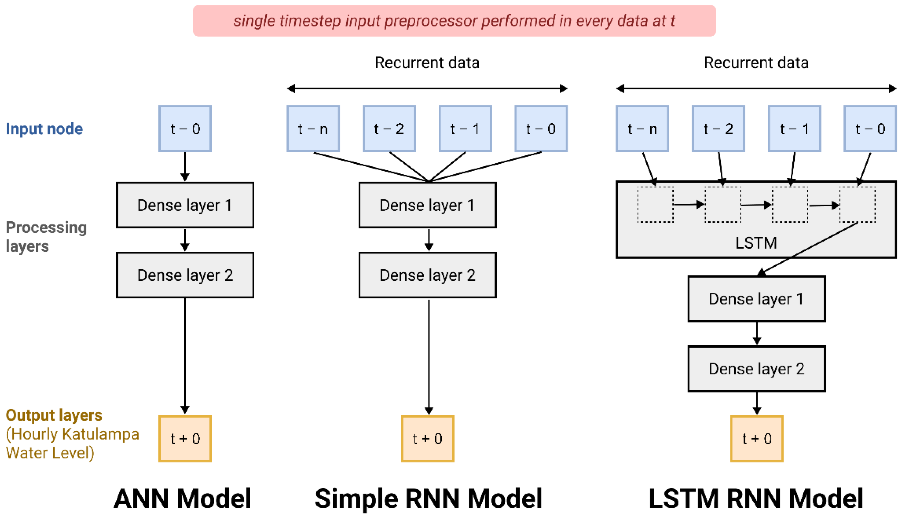
Figure 4 shows the model schematic used in this study. ANN model and simple RNN model comprised two dense layers and one output layer, with the difference in the input nodes. The simple RNN model would input data recurrently, while each datum is only read once in the standard ANN model. The difference between simple RNN and LSTM-RNN is on how the models process recurrent data: simple RNN would process multiple recurrent data in one go as a single-flow process, while the LSTM RNN model process multiple recurrent data in a directed graph along the temporal sequence, i.e., from t − n, t − n + 1, t − n + 2, all the way to t − 0. Another difference between Simple RNN and LSTM RNN used in this study is the presence of “memory cells” in LSTM. The memory cells can maintain their state over time along the temporal sequence, instead of processing all recurrent data in one go as a single-flow-process and non-linear gate unit that regulates the transmission of information from one-time series to another [25,62]. The architecture of the simple RNN is identical to the ANN model, with only differences in the simple RNN intake t − n into t − 0 recurrent data as one-big-array, and the ANN model only intakes t − 0 input array.
The NN configuration used in this study has two hidden layers and one output layer, where the activation function used in each hidden layer is ReLU (Rectified Linear Unit), with HeNormal initialization [63]. The maximum number of hidden layer units is 16 (in the first hidden layer) and 8 (in the second hidden layer). In the simple RNN, the model’s configuration is the same as in ANN, with the difference in input data, including events at t − 1, t − 2, to t − n as needed. While in LSTM RNN, the configuration is 1 LSTM layer, followed by 1 or 2 hidden layers. A prior study mentioned that although more hidden layers provide better model performance, three or more hidden layers cost more complexity than the slight performance benefit [64]. Regarding the type of hidden layer note, the prior study has mentioned that ReLU is superior to other activation function choices, e.g., linear, sine, and hyperbolic tangent functions [64]. The number of LSTM units used varies from 30 to 300, depending on the input variables’ dimensions and the optimal configuration obtained. The number of nodes in hidden layers after the LSTM RNN is adjusted based on model complexity and performance optimization, which is 2n, with n varying from 2 to 7. All models have one output layer, the predicted hourly water level at Katulampa.
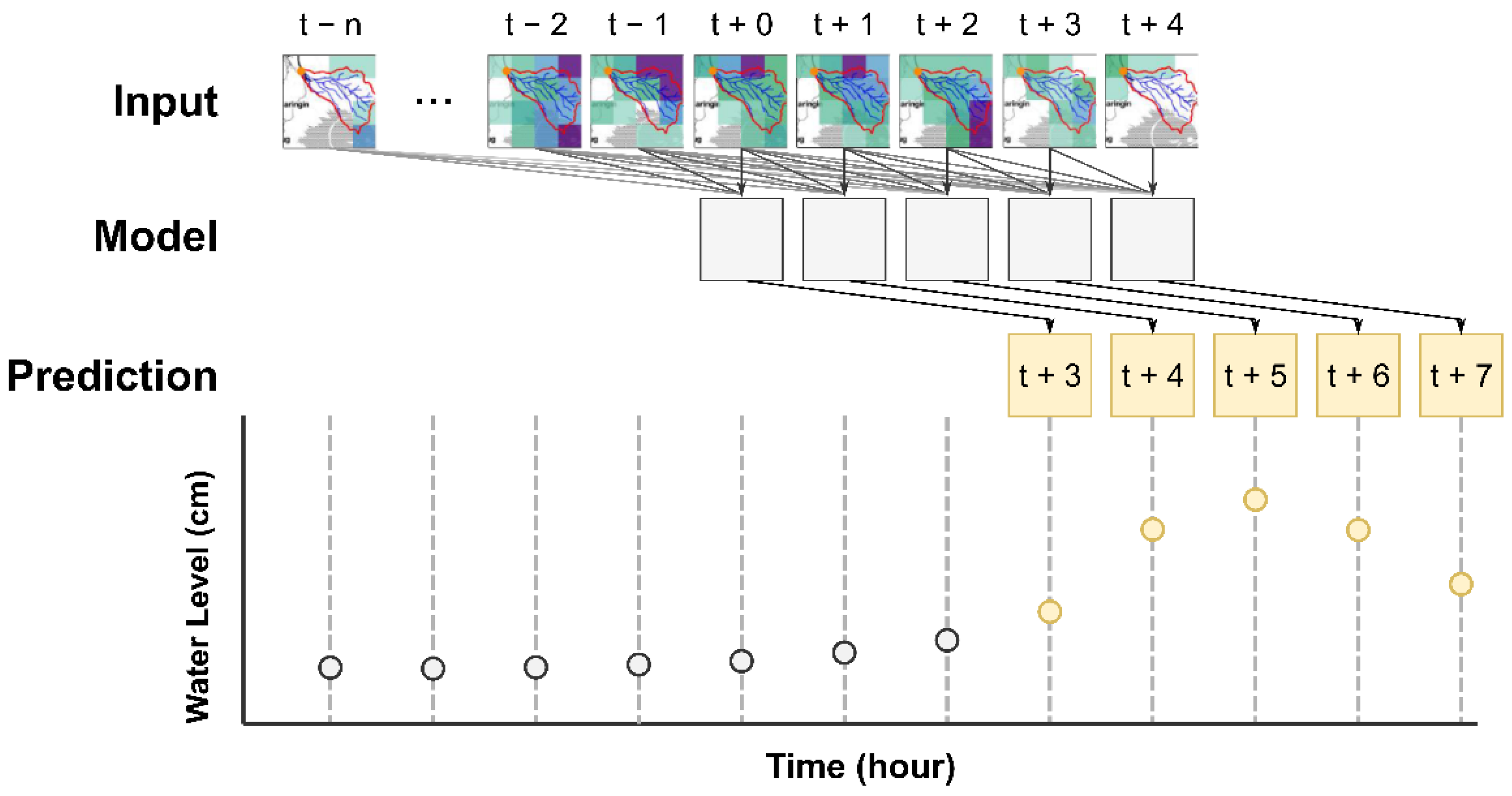
The available paired data are divided into two parts: the training set and the testing set with a proportion of 70% and 30%. Prior studies recommend such training-testing split, as it had a higher accuracy when compared to other split methods [64,65,66]. The data set is randomized before being divided into two parts (train and test). This randomized data also applies to the Simple RNN and RNN LSTM data sets. The dense layer activation function is set to ReLU [67]. The loss function was calculated using mean squared error, and the model was optimized using the Adam optimization algorithm [68]. Any hyperparameters or settings not defined in this paper are set to default in the TensorFlow machine learning framework [69]. The evaluation criteria used in this study is the R2 value. Chicco et al. [70] recommend using R2 as a standard metric “to evaluate regression analyses in any scientific domain” as it is “informative and truthful” and “does not have the interpretability limitations of MSE, RMSE, MAE, and MAPE”. The analysis is then followed by the demonstration of the capability of the NN optimizer to predict water levels in the future. Figure 5 shows the scheme of the NN-based forecast. The “t + 0 forecast” means the NN model is used to predict the current water level value, while the “t + 3 forecast” means that the model is used to predict the water level value three hours ahead. For example, a “t + 3” model prediction made at 8:00 a.m. predicts water level at 11:00 a.m. The notation differs from “t − n,” which means a prediction is made using data from the current time (t) up to x hours ago. For example, a “t − 6” recurrent model for “t + 2” flow made at 8:00 a.m. predicts water level at 10:00 a.m. using satellite data from 2:00 a.m. to 8:00 a.m.

3. Results

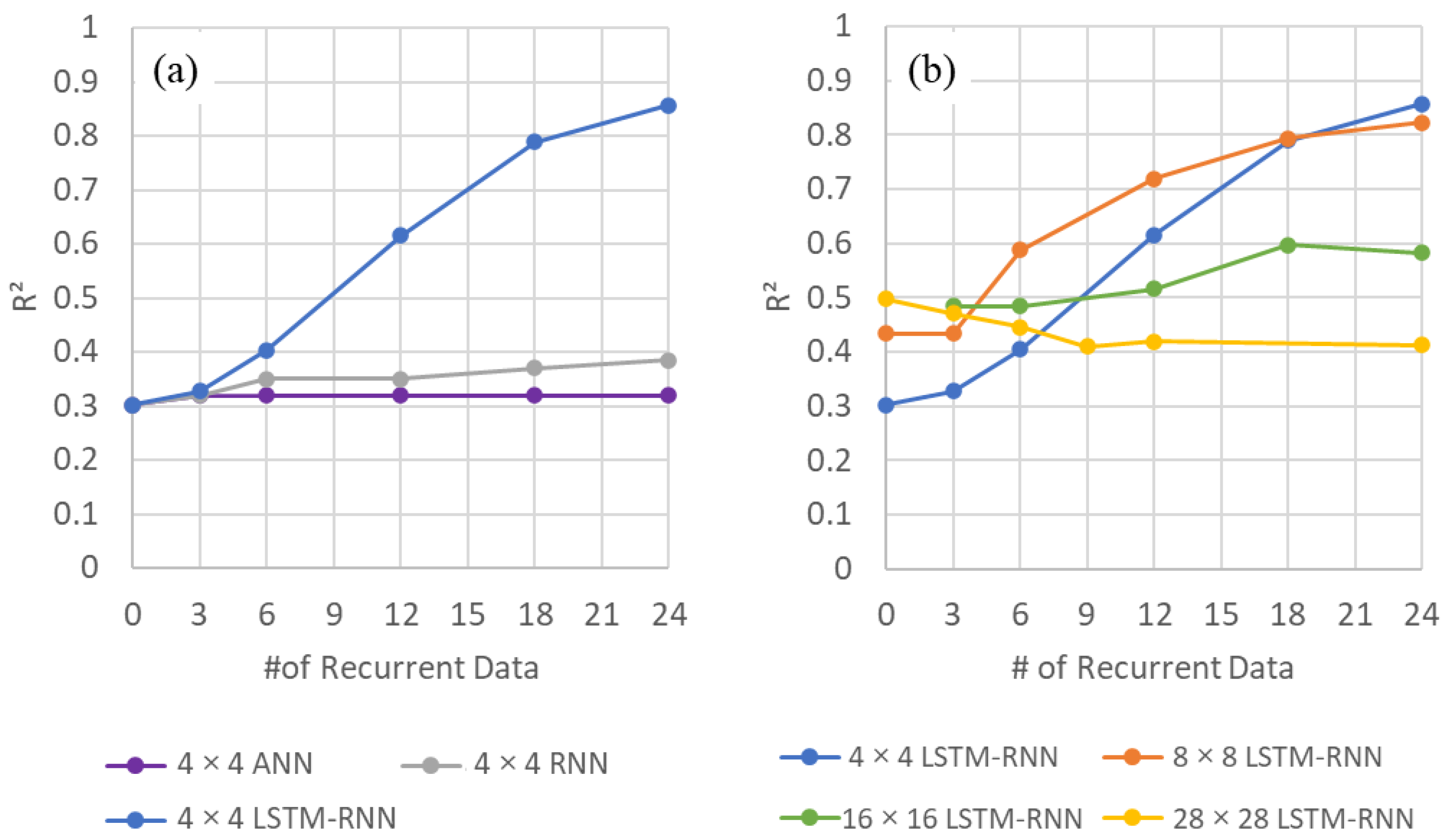
Figure 6a shows ANN, RNN, and LSTM-RNN’s performance comparison for 4 × 4 spatial extents. The figure shows the performance of RNN/LSTM neural networks to predict Katulampa water level using a different number of recurrent data, as shown on the x-axis. The number shows that the optimizer uses up to x-hours of satellite data to predict Katulampa’s water level at time t, hence, the t-n notation. As shown, a 4 × 4 ANN model is relatively insensitive to the change of the number of past data involved. Using simple RNN, the model shows performance increase as the recurrent data in longer. However, the performance value is under 0.4, even with the t − 24 model. The performance of the LSTM-RNN, on the other hand, stunted the prior two methods. Even at t − 18 data, the 4 × 4 LSTM-RNN model could reach an R2 of 0.8. Figure 6b shows the spatial optimization results on four variations of input extents: 4 × 4, 8 × 8, 16 × 16, and 28 × 28. The rationale for choosing the 4 × 4 extent is the minimum set of adjacent cells covering the entirety of the Upper Ciliwung Catchment (Figure 3). The extents were expanded to 8 × 8, 16 × 16, and 28 × 28. The largest bounding box covers the distance between the northern and southern ends of Java Island. The different extents were used to compare the effect of the number of data on the prediction performance.
Figure 6b shows that the 4 × 4 extents performed poorly when using fewer than 18 recurrent data but performed well if using more than that, with the 24-recurrent data giving an R2 value of 0.86. In the 8 × 8 configuration, using 3-h of recurrent data, the model performs better than the 4 × 4 configuration. As the number of recurrent data increases, the performance of the 8 × 8 model is consistently better than the 4 × 4 model up to 18 recurrent data. Using 24 recurrent data, the performance of 4 × 4 extent was better. In contrast to the well-performing 4 × 4 and 8 × 8 extents, the 16 × 16 and 28 × 28 extents perform poorly. Although both started better than 4 × 4 and 8 × 8 at three hours of recurrent data, as the number of recurrent data increases, both performances of 16 × 16 and 28 × 28 models drop significantly. For the 16 × 16 extent, the simulation results for three recurrent data showed promising results, giving an R2 of 0.48, higher than the R2 value of the 4 × 4 extent (0.40), while slightly lower than the other 8 × 8’s performance (0.59). However, the simulation results at 6, 9, and 12 recurrent data only increased from 0.48 at three recurrent data to 0.52, 0.55, and 0.60, respectively. Performance at 6 recurrent data is even lower than the 8 × 8 extent. The 28 × 28 extent did not give a favorable result, with more than three recurrent data leading to poorer model performance.
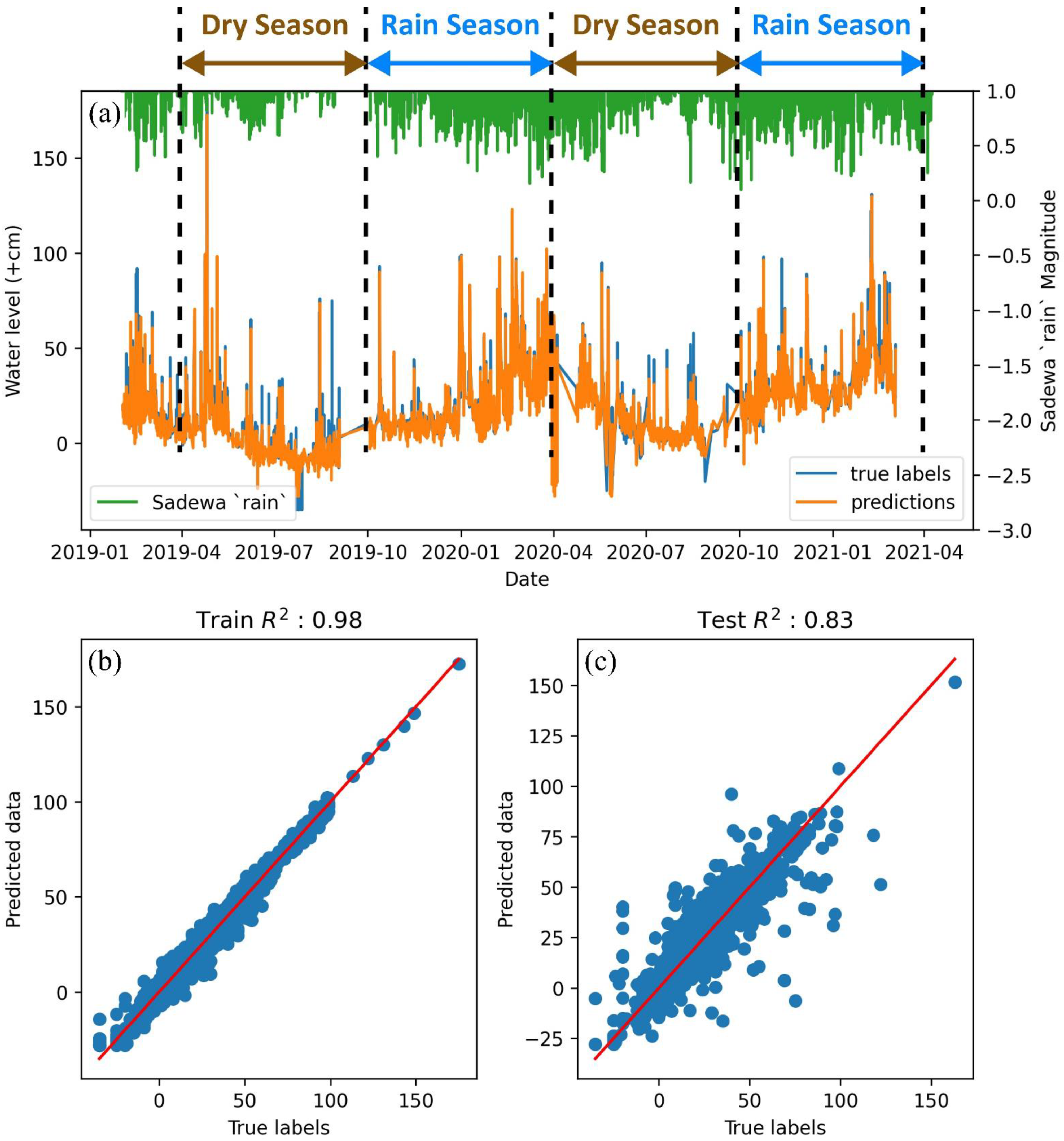
Taking 4 × 4 extent at 24 recurrent data as the snapshot, Figure 7 compares true labels (Katulampa water record levels) and LSTM RNN-predicted water levels. Figure 7a shows the timeseries comparison, with the blue line denoting the recorded Katulampa water levels, i.e., the true labels, while the orange line denotes the LSTM RNN-predicted water level. Sadewa’s rainfall variable is added to show that rainfall visually correlates with the subsequent flows, both in the observed and simulated values. Figure 7a also shows that the LSTM-RNN model could simulate flows both in the rainy and dry seasons. Low water level and low rainfall is expected in dry conditions (April–September). The predicted value also increases during the rainy season, caused by water retention in the watershed (October–March). Figure 7b shows the scatterplot comparing predicted data versus the true labels for the training dataset. As shown, the LSTM-RNN engine produced excellent training performance with an R2 of 0.98. Figure 7c shows the scatterplot comparing predicted data versus the true labels for the testing dataset, with an R2 of 0.83.
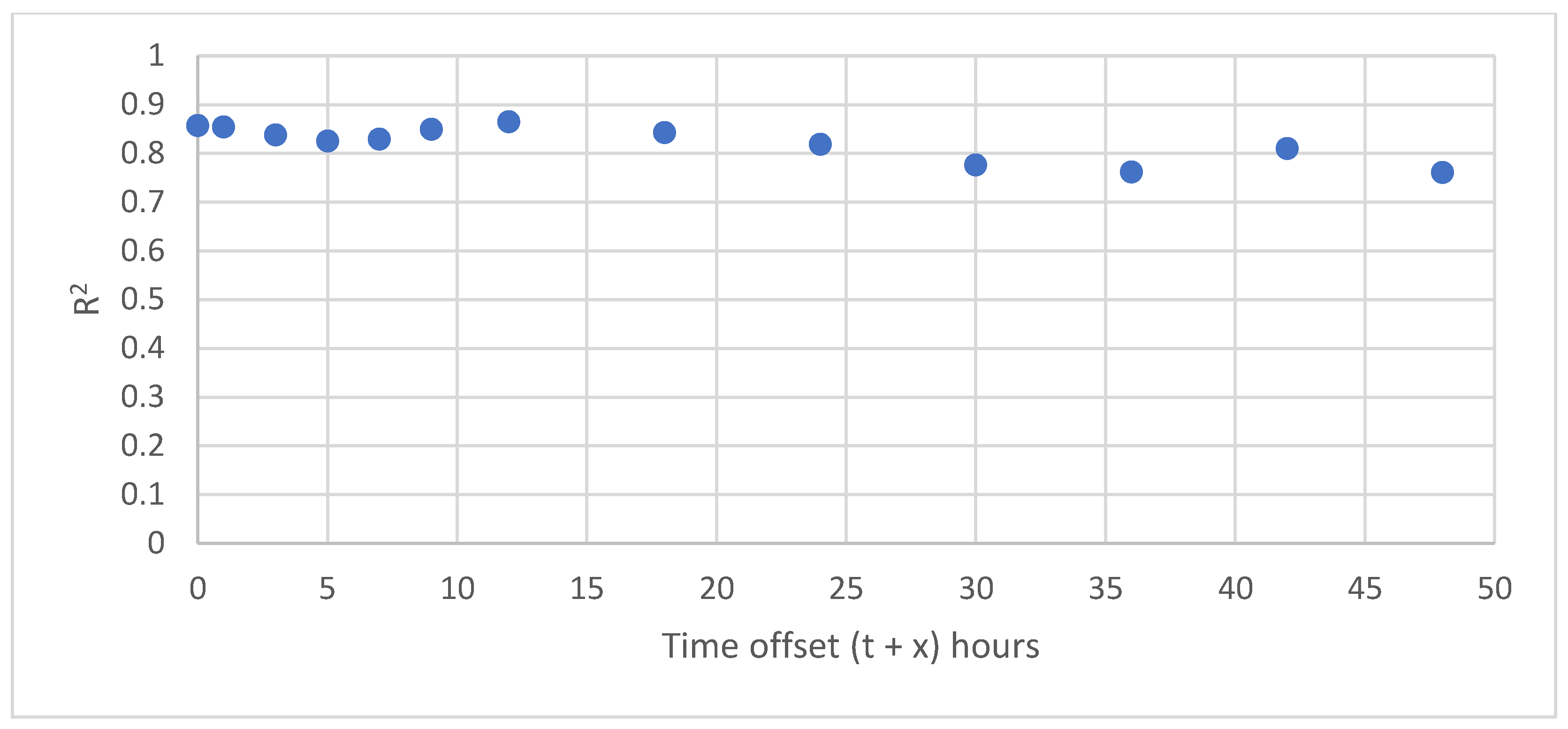
Figure 8 shows that the model could maintain an R2 performance of more than 0.85 for the next 12 h. With a predictable decrease for the next 24 h, the model can still explain 80% of the discharge events. This R2 decrease occurs at a rate of 0.0018 for every 1-h increment of the forward time domain. Prior studies [18,48] discussed such behavior, discussing that as the system tries to predict further into the future, the system then becomes more complex, and it is progressively more expensive to make an accurate prediction.

4. Discussion

The results show that LSTM performance was far better than ANN and the regular RNN. This behavior is due to a part of the LSTM called the “memory cell”, which can maintain its state over time, and a nonlinear gate unit that regulates the transmission of information from one-time series to another [25,62,71]. In the regular ANN, the information for the time step t is only used once; therefore, assuming each time step is independent of the other. However, hydrologic systems are known to have temporal dependence. This discrepancy in the underlying concept is reflected in the disability of ANNs to predict Katulampa Barrage’s water level. For the regular RNN and LSTM-RNN, although both include recurrent time steps in their training, which explicitly account for past system values, the presented result shows that the regular RNN was unable to predict the Katulampa system well. The LSTM-RNN has a “forget gate” mechanism that enables the neural networks to rhythmically forget the information the model does not need [72], allowing the prediction algorithm to filter the information it needs to predict the data given selectively.
Various studies have investigated the power of LSTMs for various hydrological and meteorological problems. The model also successfully simulates flows in the rainy and dry seasons without being explicitly programmed to simulate such distinction. The behavior of this model is interesting to note because although there are no input variables that specifically model the physical behavior on land related to seasons, the model used successfully recognizes minor abstractions among the existing data and considers this into the predicted results. This behavior is due to the LSTM’s memory cells having the capacity to retain information of gradual change both in long-term and short-term spans [71]. As [72] mentioned, the LSTM-RNN is equipped with forget gates capable of developing internal oscillations, allowing the recognition of rhythmic periodical patterns. In this case study, the periodic short-term span is the rainfall-runoff response, while the long-term one is the seasonal variation.
On the discussion regarding Sadewa data extents, the initial thought was that a more extensive extent could provide better performance with fewer recurrent data; however, the figure suggests differently. Figure 6 explains that LSTM-RNN at 0 number of recurrent data, i.e., practically plain ANN without any recurrent cells or memory cells, having a larger extent translates to better accuracy. As shown, 28 × 28 gives a 0.50 R2 value, while 8 × 8 gives a 0.43 R2 value, and 4 × 4 gives a 0.30 R2 value. However, all these values are low. Expanding the data input domain to include a t − 6 number of recurrent data increases performances for the 4 × 4 and 8 × 8 models while counterintuitively decreasing the performance of the 28 × 28 model. Further increase in the number of recurrent data (t − 12, t − 18, and t − 24) monotonically yields a performance increase for the 4 × 4 and 8 × 8 models; however, the 28 × 28 model’s R2 dip as low as 0.41. The finding could indicate that the current model could not process that many data, which is in line with findings and recommendations presented by the previous studies [64,73], indicating the 28 × 28 model extent could have too many connection weights. Too many connection weights in a model could hinder the search optimization process, trapping the model in the local optima or at the saddle points [74].
As Katulampa Barrage issues extreme weather warnings whenever the water level is above 80 cm, the current model could not predict some of these extreme discharge events despite the demonstrated ability to predict water level. The rough appearance that gives the RNN model significant advantages over the ANN model still leaves the need to refine the model, especially in high water level reproduction. Of the 26 discharge events above +80 cm in the test set, 15 events were unpredictable in an interval of one standard deviation. Additional simulations using more sophisticated methods are needed to prove the model’s effectiveness—for example, using a modified LSTM model, e.g., wavelet LSTM (WLSTM) and convolutional LSTM (CLSTM) [25]. WLSTM extensively uses the discrete wavelet transform technique, which decomposes timeseries data, thus reduces the computational cost and subsequently improves the search algorithm to find better prediction performance. CLSTM employs a stack of convolutional layers to capture the temporal properties of variables. The convolutional layers can adapt to more data being fed in training the CLSTM models, thus providing a richer the representation of the input data and the better the forecast outcomes. Another way to improve the model is by reducing the number of variables. The correlation between these variables can also be used as an initial “filter” to narrow the “optimal point search space”. Rohmat et al. [64] explained that out of the fourteen variables used in their study, three variables (canal elevation, water level elevation, and buffer zone elevation) were highly correlated with each other, then two out of three variables were ruled out in their modeling.
Based on the simulation results, the LSTM RNN model with input extents of 4 × 4 extent, 24 recurrent data (t − 24) could predict Katulampa Water Level at the current time (t + 0) with a coefficient of determination reaching 0.86 (Figure 6b). This is particularly reached with the 4 × 4 configuration using 24 recurrent data. The 8 × 8 (t − 24) performed almost the same performance (R2 = 0.82) while using a larger extent. In terms of predicting future water levels, the simulation can maintain an R2 value above 0.80 up to 24 h from the simulation time (t + 24). As one of Jakarta’s essential early warning system points, such an increase in the prediction lead time at the Katulampa Barrage poses a high importance in preparing the flood impact measure at the Manggarai Water Gate in Jakarta.
The advantages of this implementation of LSTM-RNN include the increase of lead time at the cost of short computation time while using already provisioned datasets, i.e., LAPAN’s Sadewa and Jakarta Department of Water Resources (DWR) water level data. Compared to other considerable alternatives, e.g., doppler-based radar for flood prediction, satellite-based prediction does not require a new device and system commissioning. In terms of computation time, although training the prediction takes a significant amount of time, the runtime of a trained model only takes minutes. This benchmark time was run on a lab-scale PC, indicating that it would run faster if the model were deployed on a government computer server. In terms of implementation, there are many governmental agencies interested in deploying such satellite-based flood prediction systems, namely Jakarta DWR, the Ministry of National Development Planning of the Republic of Indonesia, and the Ministry of Public Works and Housing of the Republic of Indonesia. The ministries do not only have an interest in applying such a method in Jakarta but also other places in Indonesia.
Regarding the limitation of this study, it is essential to highlight that the scope of this study is only up to Katulampa Barrage; thus, the developed model may be specific to the characteristics of the Upper Ciliwung Catchment. If the model were to be implemented in another region, adjustments must be made. The currently presented Upper Ciliwung Catchment model performs well at 4 × 4 and 8 × 8 extents for the spatial extent. If the model were implemented elsewhere, the extent used is preferably the smallest bounding box covering the entire studied watershed. This recommendation is for the model to converge quicker. The formula of “t − n recurrent data to predict t + x water level” using the same LSTM-RNN can be used as long as the water level data at the interest location is available. If the formula were to be adjusted, the number of recurrent data could also be related to other location-sensitive variables, e.g., ground-based climate measurements, rainfall time of concentration, land-cover coefficient, and watershed geometry.
The model configurations, e.g., hidden layer configurations, could also be adjusted to the complexity of the variables at the location—for example, in the locations where human interference plays a significant role, e.g., a catchment with intensive irrigation practice or a catchment with a regulated reservoir operation. Rohmat et al. [64] present that the scenarios related to humans (referred to as “management scenarios”) can be explicitly included as the input variables. Developments to locations with poor water level data can also be carried out using transfer learning. Transfer learning is where situations learned in one setting, e.g., the P1 distribution, can be exploited to increase generalization in another set, e.g., the P2 distribution [75]. In the hydrological domain, models that have previously been trained in one location can be transferred to different catchments, either by generalizing or adjusting the complexity to predict a certain water level measurement point with few good quality measurement points [38]. While the current model has incorporated temporal memory through the LSTM memory cells’ mechanism (which includes cumulative rainfall over the recurrent data span), soil moisture content could also be a valuable new variable to improve the LSTM-RNN model further. The initial soil moisture content significantly impacts the infiltration process [76], making it one of the essential factors in rainfall-runoff generation. Although the Sadewa dataset currently does not include a soil moisture variable, many other remotely sensed sources can be utilized for future studies [77].

5. Conclusions

The water level observation of the Upper Ciliwung River by the Katulampa Barrage is crucial in decreasing the risk of flooding in Jakarta, particularly in areas where the Ciliwung River flows. The highest flow measured in the barrage would take 13–14 h to reach the city’s center, giving officials and citizens enough time to prepare for the flood risk. However, given Jakarta’s ever-increasing vulnerability to floods, a more advanced early warning system with a longer forecasting lead time is required. In this study, LAPAN’s Sadewa data is utilized to predict the water level of Katulampa Barrage using LSTM-RNN. The Katulampa Watershed is completely contained within the 4 × 4 Sadewa cell boundaries. Three larger extents are also considered, i.e., 8 × 8, 16 × 16, and 28 × 28, which the last extent spans over the north-south length of Java Island. Each cell of the Sadewa dataset is a 0.05 × 0.05 decimal degrees cell with an approximate area of 30.8 km2. The result compares prediction performance between ANN, RNN, and LSTM-RNN, with the first two unable to accurately predict the water level.
Using LSTM-RNN, the model could accurately predict Katulampa’s water level using the 4 × 4 and 8 × 8 extents with recurrent t − 24 h of data, with an R2 above 0.82. In forecasting, the model was able to maintain R2 above 0.80 up to 24 h into the future. The finding provides the potential for the Sadewa-fed LSTM-RNN prediction of Katulampa Barrage’s water level accurately to increase the forecast lead time. Such an increase would be beneficial to improve the region’s preparedness for incoming floods, considering the ever-increasing vulnerability of Jakarta City. In terms of the potential of implementation, several governmental agencies seek to implement such technology, both for implementation in Jakarta and the other regions in Indonesia. There are considerations for adjustments for the method’s implementation in another region. It is recommended to use the smallest bounding extent that covers the studied watershed to promote better performance and faster convergence for the satellite data extent. If anthropogenic management rules significantly influence the study area, including such rules in the modeling is preferred. For future development, the actual deployment, testing, and public evaluation of the model can be pursued to evaluate the model’s applicability in a real-case situation. Another future direction is that the current model can be extended to generalize better to other watersheds. Implementing more sophisticated and well-generalizing LSTM engines, e.g., WLSTM and CLSTM, could also be pursued for their ability to transform past and future patterns into parametric wave functions (WLSTM) or a hierarchical structure of the data (CLSTM).

Author Contributions

Conceptualization, H.K. and F.I.W.R.; methodology, H.K.; software, J.R.V.; validation, H.K., J.R.V. and F.I.W.R.; formal analysis, H.K.; investigation, J.R.V.; resources, M.S.B.K.; data curation, J.R.V.; writing—original draft preparation, J.R.V.; writing—review and editing, H.K. and F.I.W.R.; visualization, J.R.V. and F.I.W.R.; supervision, M.S.B.K.; project administration, M.S.B.K.; funding acquisition, M.S.B.K. All authors have read and agreed to the published version of the manuscript.

Funding

This research was funded by the Institut Teknologi Bandung (ITB) Research Excellence Fund 2021 (Riset Unggulan ITB 2021), the ITB Ganesha Talent Assistantship Program, and the ITB DTTP research grant for the contract number 1354/IT1.B05/KP/2021. The APC was funded by FTSL (FCEE) ITB Research Publication grant 2022.

Institutional Review Board Statement

Not applicable.

Informed Consent Statement

Not applicable.

Data Availability Statement

Restrictions apply to the availability of these data. Data was obtained from LAPAN-BRIN (Indonesian Aerospace Agency—National Research and Innovation Agency) and are available with the permission of LAPAN-BRIN.

Acknowledgments

We acknowledge Wendi Harjupa ([email protected]) of LAPAN-BRIN for the help in acquiring and understanding the Sadewa satellite data.

Conflicts of Interest

The authors declare no conflict of interest.

References

  1. Indonesian National Board for Disaster Management—BNPB. Disaster Events in 2020—Kejadian Bencana Tahun 2020; BNPB: Jakarta, Indonesia, 2021.
  2. Cahya, G.H. Climate Change Cause of Greater Jakarta Floods, BMKG Says. Available online: https://www.thejakartapost.com/news/2020/02/26/climate-change-behind-2020-floods-that-displaced-thousands-in-jakarta-agency-says.html (accessed on 17 April 2022).
  3. Farid, M.; Pusparani, H.H.; Kusuma, M.S.B.; Natasaputra, S. Study on Effectiveness of Flood Control Based on Risk Level: Case Study of Kampung Melayu Village and Bukit Duri Village. Proc. MATEC Web Conf. 2017, 101, 5003. [Google Scholar] [CrossRef]
  4. Moe, I.R.; Kure, S.; Januriyadi, N.F.; Farid, M.; Udo, K.; Kazama, S.; Koshimura, S. Future Projection of Flood Inundation Considering Land-Use Changes and Land Subsidence in Jakarta, Indonesia. Hydrol. Res. Lett. 2017, 11, 99–105. [Google Scholar]
  5. Fuchs, R.J. Cities at Risk: Asia’s Coastal Cities in an Age of Climate Change; East-West Center: Honolulu, HI, USA, 2010. [Google Scholar]
  6. Mishra, B.K.; Rafiei Emam, A.; Masago, Y.; Kumar, P.; Regmi, R.K.; Fukushi, K. Assessment of Future Flood Inundations under Climate and Land Use Change Scenarios in the Ciliwung River Basin, Jakarta. J. Flood Risk Manag. 2018, 11, S1105–S1115. [Google Scholar] [CrossRef]
  7. Liu, J.; Doan, C.D.; Liong, S.Y.; Sanders, R.; Dao, A.T.; Fewtrell, T. Regional Frequency Analysis of Extreme Rainfall Events in Jakarta. Nat. Hazards 2015, 75, 1075–1104. [Google Scholar] [CrossRef]
  8. Emam, A.R.; Mishra, B.K.; Kumar, P.; Masago, Y.; Fukushi, K. Impact Assessment of Climate and Land-Use Changes on Flooding Behavior in the Upper Ciliwung River, Jakarta, Indonesia. Water 2016, 8, 559. [Google Scholar] [CrossRef] [Green Version]
  9. Formánek, A.; Silasari, R.; Kusuma, M.S.B.; Kardhana, H. Two-Dimensional Model of Ciliwung River Flood in DKI Jakarta for Development of the Regional Flood Index Map. J. Eng. Technol. Sci. 2013, 45, 307–325. [Google Scholar] [CrossRef] [Green Version]
  10. Jones, P. Formalizing the Informal: Understanding the Position of Informal Settlements and Slums in Sustainable Urbanization Policies and Strategies in Bandung, Indonesia. Sustainability 2017, 9, 1436. [Google Scholar] [CrossRef] [Green Version]
  11. Statistics Indonesia. Statistical Yearbook of Indonesia 2021; Statistics Indonesia: Jakarta, Indonesia, 2021.
  12. Widyasamratri, H.; Souma, K.; Suetsugi, T. Study of Urban Temperature Profiles on the Various Land Cover in the Jakarta Metropolitan Area, Indonesia. Indones. J. Geogr. 2019, 51, 357–363. [Google Scholar] [CrossRef] [Green Version]
  13. Wahyudi, A.; Liu, Y.; Corcoran, J. Combining Landsat and Landscape Metrics to Analyse Large-Scale Urban Land Cover Change: A Case Study in the Jakarta Metropolitan Area. J. Spat. Sci. 2018, 64, 515–534. [Google Scholar] [CrossRef]
  14. Zhu, J.; Simarmata, H.A. Formal Land Rights versus Informal Land Rights: Governance for Sustainable Urbanization in the Jakarta Metropolitan Region, Indonesia. Land Use Policy 2015, 43, 63–73. [Google Scholar] [CrossRef]
  15. Simone, A.M.; Abdou, M. Jakarta, Drawing the City Nea; University of Minnesota Press: Minneapolis, IN, USA, 2014; p. 334. [Google Scholar]
  16. Van Voorst, R. Juxtapositions in Jakarta: How Flood Interventions Reinforce and Challenge Urban Divides. Urban Forum 2020, 31, 373–388. [Google Scholar] [CrossRef]
  17. Ginting, S.; Putuhena, W.M. Sistem Peringatan Dini Banjir Jakarta (Jakarta Flood Early Warning System, J-FEWS). J. Sumber Daya Air 2014, 10, 71–84. [Google Scholar]
  18. Powers, J.G.; Klemp, J.B.; Skamarock, W.C.; Davis, C.A.; Dudhia, J.; Gill, D.O.; Coen, J.L.; Gochis, D.J.; Ahmadov, R.; Peckham, S.E.; et al. The Weather Research and Forecasting Model: Overview, System Efforts, and Future Directions. Bull. Am. Meteorol. Soc. 2017, 98, 1717–1737. [Google Scholar] [CrossRef]
  19. Skamarock, W.C.; Klemp, J.B. A Time-Split Nonhydrostatic Atmospheric Model for Weather Research and Forecasting Applications. J. Comput. Phys. 2008, 227, 3465–3485. [Google Scholar] [CrossRef]
  20. Burnash, R.J.; Ferral, R.L.; McGuire, R.A. A Generalized Streamflow Simulation System: Conceptual Modeling for Digital Computers; US Department of Commerce, National Weather Service, and State of California, Department of Water Resources: San Francisco, CA, USA, 1973. [Google Scholar]
  21. Crawford, N.H.; Thurin, S.M. Hydrologic Estimates for Small Hydroelectric Projects; Small Decentralized Hydropower Program, International Programs Division: Washington, DC, USA, 1981. [Google Scholar]
  22. Bai, Y.; Bezak, N.; Sapač, K.; Klun, M.; Zhang, J. Short-Term Streamflow Forecasting Using the Feature-Enhanced Regression Model. Water Resour. Manag. 2019, 33, 4783–4797. [Google Scholar] [CrossRef]
  23. He, X.; Luo, J.; Zuo, G.; Xie, J. Daily Runoff Forecasting Using a Hybrid Model Based on Variational Mode Decomposition and Deep Neural Networks. Water Resour. Manag. 2019, 33, 1571–1590. [Google Scholar] [CrossRef]
  24. Kabir, S.; Patidar, S.; Pender, G. Investigating Capabilities of Machine Learning Techniques in Forecasting Stream Flow. Proc. Inst. Civ. Eng. Water Manag. 2020, 173, 69–86. [Google Scholar] [CrossRef]
  25. Ni, L.; Wang, D.; Singh, V.P.; Wu, J.; Wang, Y.; Tao, Y.; Zhang, J. Streamflow and Rainfall Forecasting by Two Long Short-Term Memory-Based Models. J. Hydrol. 2020, 583, 124296. [Google Scholar] [CrossRef]
  26. Qi, Y.; Zhou, Z.; Yang, L.; Quan, Y.; Miao, Q. A Decomposition-Ensemble Learning Model Based on LSTM Neural Network for Daily Reservoir Inflow Forecasting. Water Resour. Manag. 2019, 33, 4123–4139. [Google Scholar] [CrossRef]
  27. Qin, J.; Liang, J.; Chen, T.; Lei, X.; Kang, A. Simulating and Predicting of Hydrological Time Based on TensorFlow Deep Learning. Pol. J. Environ. Stud. 2018, 28, 795–802. [Google Scholar] [CrossRef]
  28. Wang, J.H.; Lin, G.F.; Chang, M.J.; Huang, I.H.; Chen, Y.R. Real-Time Water-Level Forecasting Using Dilated Causal Convolutional Neural Networks. Water Resour. Manag. 2019, 33, 3759–3780. [Google Scholar] [CrossRef]
  29. Yuan, X.; Chen, C.; Lei, X.; Yuan, Y.; Muhammad Adnan, R. Monthly Runoff Forecasting Based on LSTM–ALO Model. Stoch. Environ. Res. Risk Assess. 2018, 32, 2199–2212. [Google Scholar] [CrossRef]
  30. Zuo, G.; Luo, J.; Wang, N.; Lian, Y.; He, X. Decomposition Ensemble Model Based on Variational Mode Decomposition and Long Short-Term Memory for Streamflow Forecasting. J. Hydrol. 2020, 585, 124776. [Google Scholar] [CrossRef]
  31. Pan, B.; Hsu, K.; AghaKouchak, A.; Sorooshian, S. Improving Precipitation Estimation Using Convolutional Neural Network. Water Resour. Res. 2019, 55, 2301–2321. [Google Scholar] [CrossRef] [Green Version]
  32. Tang, G.; Long, D.; Behrangi, A.; Wang, C.; Hong, Y. Exploring Deep Neural Networks to Retrieve Rain and Snow in High Latitudes Using Multisensor and Reanalysis Data. Water Resour. Res. 2018, 54, 8253–8278. [Google Scholar] [CrossRef] [Green Version]
  33. Chen, L.; Cao, Y.; Ma, L.; Zhang, J. A Deep Learning-Based Methodology for Precipitation Nowcasting with Radar. Earth Space Sci. 2020, 7, e2019EA000812. [Google Scholar] [CrossRef] [Green Version]
  34. Yan, Q.; Ji, F.; Miao, K.; Wu, Q.; Xia, Y.; Li, T. Convolutional Residual-Attention: A Deep Learning Approach for Precipitation Nowcasting. Adv. Meteorol. 2020, 2020, 6484812. [Google Scholar] [CrossRef]
  35. Poornima, S.; Pushpalatha, M. Prediction of Rainfall Using Intensified LSTM Based Recurrent Neural Network with Weighted Linear Units. Atmosphere 2019, 10, 668. [Google Scholar] [CrossRef] [Green Version]
  36. Wang, Q.; Huang, J.; Liu, R.; Men, C.; Guo, L.; Miao, Y.; Jiao, L.; Wang, Y.; Shoaib, M.; Xia, X. Sequence-Based Statistical Downscaling and Its Application to Hydrologic Simulations Based on Machine Learning and Big Data. J. Hydrol. 2020, 586, 124875. [Google Scholar] [CrossRef]
  37. Yang, T.; Sun, F.; Gentine, P.; Liu, W.; Wang, H.; Yin, J.; Du, M.; Liu, C. Evaluation and Machine Learning Improvement of Global Hydrological Model-Based Flood Simulations. Environ. Res. Lett. 2019, 14, 114027. [Google Scholar] [CrossRef]
  38. Kratzert, F.; Klotz, D.; Brenner, C.; Schulz, K.; Herrnegger, M. Rainfall-Runoff Modelling Using Long Short-Term Memory (LSTM) Networks. Hydrol. Earth Syst. Sci. 2018, 22, 6005–6022. [Google Scholar] [CrossRef] [Green Version]
  39. Kao, I.F.; Zhou, Y.; Chang, L.C.; Chang, F.J. Exploring a Long Short-Term Memory Based Encoder-Decoder Framework for Multi-Step-Ahead Flood Forecasting. J. Hydrol. 2020, 583, 124631. [Google Scholar] [CrossRef]
  40. Xiang, Z.; Yan, J.; Demir, I. A Rainfall-Runoff Model with LSTM-Based Sequence-to-Sequence Learning. Water Resour. Res. 2020, 56, e2019WR025326. [Google Scholar] [CrossRef]
  41. Nguyen, D.H.; Bae, D.H. Correcting Mean Areal Precipitation Forecasts to Improve Urban Flooding Predictions by Using Long Short-Term Memory Network. J. Hydrol. 2020, 584, 124710. [Google Scholar] [CrossRef]
  42. Zhang, D.; Hølland, E.S.; Lindholm, G.; Ratnaweera, H. Hydraulic Modeling and Deep Learning Based Flow Forecasting for Optimizing Inter Catchment Wastewater Transfer. J. Hydrol. 2018, 567, 792–802. [Google Scholar] [CrossRef]
  43. Ahmed, A.A.M.; Deo, R.C.; Ghahramani, A.; Feng, Q.; Raj, N.; Yin, Z.; Yang, L. New Double Decomposition Deep Learning Methods for River Water Level Forecasting. Sci. Total Environ. 2022, 831, 154722. [Google Scholar] [CrossRef]
  44. Kumar, D.; Singh, A.; Samui, P.; Jha, R.K. Forecasting Monthly Precipitation Using Sequential Modelling. Hydrol. Sci. J. 2019, 64, 690–700. [Google Scholar] [CrossRef]
  45. Wu, H.; Yang, Q.; Liu, J.; Wang, G. A Spatiotemporal Deep Fusion Model for Merging Satellite and Gauge Precipitation in China. J. Hydrol. 2020, 584, 124664. [Google Scholar] [CrossRef]
  46. Hrnjica, B.; Bonacci, O. Lake Level Prediction Using Feed Forward and Recurrent Neural Networks. Water Resour. Manag. 2019, 33, 2471–2484. [Google Scholar] [CrossRef]
  47. Zhu, S.; Hrnjica, B.; Ptak, M.; Choiński, A.; Sivakumar, B. Forecasting of Water Level in Multiple Temperate Lakes Using Machine Learning Models. J. Hydrol. 2020, 585, 124819. [Google Scholar] [CrossRef]
  48. Kesuma, T.N.A.; Saputra, D.; Farid, M.; Kusuma, M.S.B.; Kuntoro, A.A. Contribution of Manggarai Gate Improvement to Flood in Manggarai Village Based on Recorded Flood Event. IOP Conf. Ser. Earth Environ. Sci. 2021, 737, 012027. [Google Scholar] [CrossRef]
  49. Ratnaningsih, D.; Nasution, E.L.; Wardhani, N.T.; Pitalokasari, O.D.; Fauzi, R. Water Pollution Trends in Ciliwung River Based on Water Quality Parameters. IOP Conf. Ser. Earth Environ. Sci. 2019, 407, 012006. [Google Scholar] [CrossRef]
  50. Ali, M.; Hadi, S.; Sulistyantara, B. Study on Land Cover Change of Ciliwung Downstream Watershed with Spatial Dynamic Approach. Procedia Soc. Behav. Sci. 2016, 227, 52–59. [Google Scholar] [CrossRef] [Green Version]
  51. Arifasihati, Y. Kaswanto Analysis of Land Use and Cover Changes in Ciliwung and Cisadane Watershed in Three Decades. Procedia Environ. Sci. 2016, 33, 465–469. [Google Scholar] [CrossRef] [Green Version]
  52. Rachman, L.M.; Hidayat, Y.; Baskoro, D.P.T.; Noywuli, N. Simulasi Pengendalian Debit DAS Ciliwung Hulu Dengan Menggunakan Model SWAT. In Proceedings of the Seminar Nasional Pengelolaan Daerah Aliran Sungai Secara Terpadu, Pekanbaru, Indonesia, 27 November 2017; pp. 291–304. [Google Scholar]
  53. Farid, M.; Saputra, D.; Maitsa, T.R.; Kesuma, T.N.A.; Kuntoro, A.A.; Chrysanti, A. Relationship between Extreme Rainfall and Design Flood-Discharge of the Ciliwung River. IOP Conf. Ser. Earth Environ. Sci. 2021, 708, 012031. [Google Scholar] [CrossRef]
  54. Pratama, M.I.; Rohmat, F.I.W.; Farid, M.; Adityawan, M.B.; Kuntoro, A.A.; Moe, I.R. Flood Hydrograph Simulation to Estimate Peak Discharge in Ciliwung River Basin. IOP Conf. Ser. Earth Environ. Sci. 2021, 708, 012028. [Google Scholar] [CrossRef]
  55. Yatsrib, M.; Harman, A.N.; Taufik, S.R.; Kesuma, T.N.A.; Saputra, D.; Kusuma, M.S.B.; Farid, M.; Kuntoro, A.A. Study on the Contribution of Normalization to Reducing Flood Risk in the Ciliwung River, Tebet District, Jakarta. IOP Conf. Ser. Earth Environ. Sci. 2021, 933, 012032. [Google Scholar] [CrossRef]
  56. Van Voorst, R. Formal and Informal Flood Governance in Jakarta, Indonesia. Habitat Int. 2016, 52, 5–10. [Google Scholar] [CrossRef]
  57. Research Center for Atmospheric Technology LAPAN-BRIN Sadewa (Satellite-Based Disaster Early Warning System). Available online: https://sadewa.sains.lapan.go.id/ (accessed on 19 January 2022).
  58. Nafiisyanti, A. Pembaharuan Aplikasi Peringatan Bencana Dini: Sadewa. Media Dirgant. 2014, 9, 2. [Google Scholar]
  59. DKI Jakarta Water Resources Service Tinggi Muka Air Online|Dinas Sumber Daya Air Provinsi DKI Jakarta. Available online: http://poskobanjirdsda.jakarta.go.id/ (accessed on 19 January 2022).
  60. Agatonovic-Kustrin, S.; Beresford, R. Basic Concepts of Artificial Neural Network (ANN) Modeling and Its Application in Pharmaceutical Research. J. Pharm. Biomed. Anal. 2000, 22, 717–727. [Google Scholar] [CrossRef]
  61. Sit, M.; Demiray, B.Z.; Xiang, Z.; Ewing, G.J.; Sermet, Y.; Demir, I. A Comprehensive Review of Deep Learning Applications in Hydrology and Water Resources. Water Sci. Technol. 2020, 82, 2635–2670. [Google Scholar] [CrossRef] [PubMed]
  62. Hu, R.; Fang, F.; Pain, C.C.; Navon, I.M. Rapid Spatio-Temporal Flood Prediction and Uncertainty Quantification Using a Deep Learning Method. J. Hydrol. 2019, 575, 911–920. [Google Scholar] [CrossRef]
  63. He, K.; Zhang, X.; Ren, S.; Sun, J. Delving Deep into Rectifiers: Surpassing Human-Level Performance on ImageNet Classification. In Proceedings of the 2015 IEEE International Conference on Computer Vision (ICCV), Santiago, Chile, 7–13 December 2015; pp. 1026–1034. [Google Scholar]
  64. Rohmat, F.I.W.; Labadie, J.W.; Gates, T.K. Deep Learning for Compute-Efficient Modeling of BMP Impacts on Stream- Aquifer Exchange and Water Law Compliance in an Irrigated River Basin. Environ. Model. Softw. 2019, 122, 104529. [Google Scholar] [CrossRef]
  65. Gholamy, A.; Kreinovich, V.; Kosheleva, O. Why 70/30 or 80/20 Relation between Training and Testing Sets: A Pedagogical Explanation; Departmental Technical Reports (CS) UTEP-CS-18-09; University of Texas: Austin, TX, USA, 2018. [Google Scholar]
  66. Adelabu, S.; Mutanga, O.; Adam, E. Testing the Reliability and Stability of the Internal Accuracy Assessment of Random Forest for Classifying Tree Defoliation Levels Using Different Validation Methods. Geocarto Int. 2015, 30, 810–821. [Google Scholar] [CrossRef]
  67. Szandała, T. Review and Comparison of Commonly Used Activation Functions for Deep Neural Networks. Stud. Comput. Intell. 2021, 903, 203–224. [Google Scholar] [CrossRef]
  68. Kingma, D.P.; Ba, J.L. Adam: A Method for Stochastic Optimization. In Proceedings of the International Conference on Learning Representations 2015, San Diego, CA, USA, 7–9 May 2015; pp. 1–15. [Google Scholar] [CrossRef]
  69. Abadi, M.; Barham, P.; Chen, J.; Chen, Z.; Davis, A.; Dean, J.; Devin, M.; Ghemawat, S.; Irving, G.; Isard, M.; et al. TensorFlow: A System for Large-Scale Machine Learning; USENIX: Berkeley, CA, USA, 2016; Volume 10, ISBN 978-1-931971-33-1. [Google Scholar]
  70. Chicco, D.; Warrens, M.J.; Jurman, G. The Coefficient of Determination R-Squared Is More Informative than SMAPE, MAE, MAPE, MSE and RMSE in Regression Analysis Evaluation. PeerJ Comput. Sci. 2021, 7, e623. [Google Scholar] [CrossRef]
  71. Hochreiter, S.; Schmidhuber, J. Long Short-Term Memory. Neural Comput. 1997, 9, 1735–1780. [Google Scholar] [CrossRef]
  72. Gers, F.A.; Schmidhuber, J.; Cummins, F. Learning to Forget: Continual Prediction with LSTM. Neural Comput. 2000, 12, 2451–2471. [Google Scholar] [CrossRef]
  73. Wu, W.; Dandy, G.C.; Maier, H.R. Protocol for Developing ANN Models and Its Application to the Assessment of the Quality of the ANN Model Development Process in Drinking Water Quality Modelling. Environ. Model. Softw. 2014, 54, 108–127. [Google Scholar] [CrossRef]
  74. Dauphin, Y.N.; Pascanu, R.; Gulcehre, C.; Cho, K.; Ganguli, S.; Bengio, Y. Identifying and Attacking the Saddle Point Problem in High-Dimensional Non-Convex Optimization. In Proceedings of the Advances in Neural Information Processing Systems 27, Montreal, QC, Canada, 8–13 December 2014; pp. 2933–2941. [Google Scholar]
  75. Goodfellow, I.; Bengio, Y.; Courville, A. Deep Learning; MIT Press: Cambridge, MA, USA, 2016. [Google Scholar]
  76. Song, S.; Wang, W. Impacts of Antecedent Soil Moisture on the Rainfall-Runoff Transformation Process Based on High-Resolution Observations in Soil Tank Experiments. Water 2019, 11, 296. [Google Scholar] [CrossRef] [Green Version]
  77. Kim, S.; Zhang, R.; Pham, H.; Sharma, A. A Review of Satellite-Derived Soil Moisture and Its Usage for Flood Estimation. Remote Sens. Earth Syst. Sci. 2019, 2, 225–246. [Google Scholar] [CrossRef]
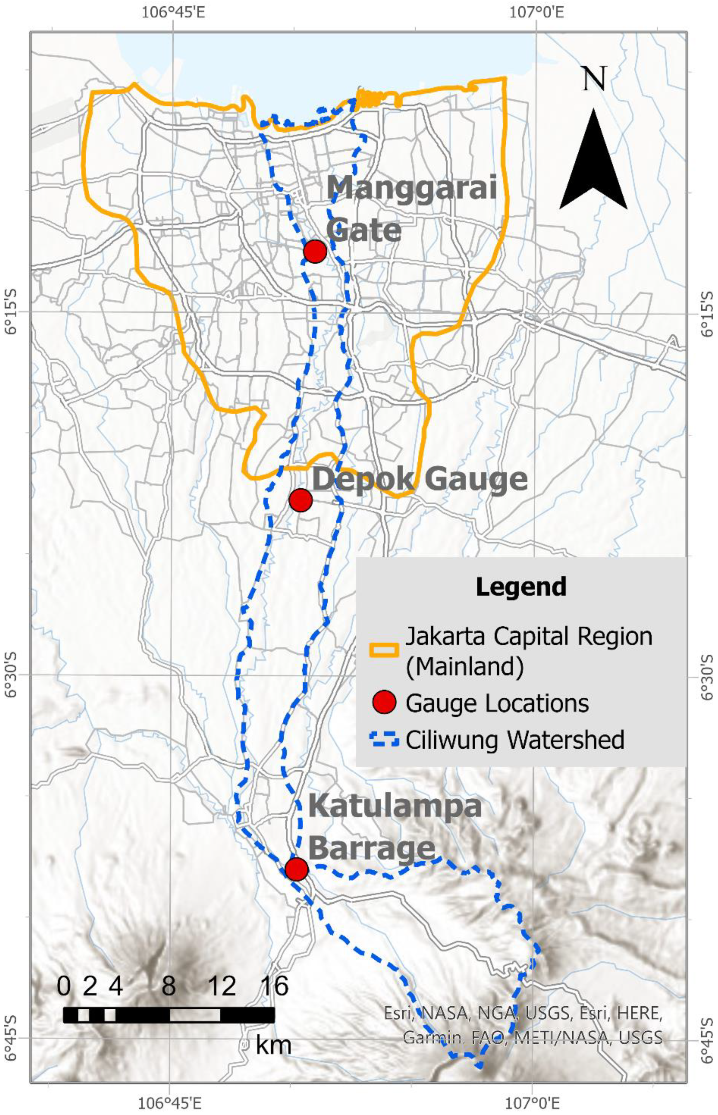
Figure 1. Study area orientation and the general conveyance time between point of interests; observed peak water level at Katulampa Barrage would reach Manggarai gate within 13–14 h, which is at the very heart of the Jakarta Capital Region.
Water 14 01469 g001
Figure 2. Illustration of the different data type usages to increase flood prediction lead time.
Water 14 01469 g002
Figure 3. Sadewa data processing extents. The colors of the dashed box boundaries represent different boundary extents.
Water 14 01469 g003
Figure 4. ANN, RNN, LSTM model schematics.
Water 14 01469 g004
Figure 5. Temporal forecasting scheme.
Water 14 01469 g005
Figure 6. Performance comparison of (a) ANN, RNN, and LSTM-RNN; (b) spatial optimization results on four variations of input extents: 4 × 4, 8 × 8, 16 × 16, and 28 × 28.
Water 14 01469 g006
Figure 7. (a) Timeseries comparison between true labels (Katulampa water record levels, blue line) and LSTM RNN-predicted water level (orange line), with Sadewa’s rainfall value as an added information; scatterplot comparing predicted data vs. true labels for (b) training and (c) testing datasets.
Water 14 01469 g007
Figure 8. Forecast performance for t + x offset versus time offset of a 4 × 4 t − 24 LSTM-RNN model.
Water 14 01469 g008
Table 1. Comparison between data source and target output variables in the resect publications in the field of machine learning-based flood prediction research. The shaded cells denote the same datatypes used for prediction source and output.
Output
RainfallDischargeWater Level
InputSatellite[31,32] [43], this research
Radar[33,34]
Meteorological[35,36][37]
Rainfall[25,44,45][38,39,40][41,42]
Discharge [22,23,24,25,26,27,28,29]
Water Level [46,47]
Table 2. Summary of the source dataset used in this study.
VariableDatasetTemporal ResolutionPublicly Available at the Time of WritingResponsible Agency
1Composite observation showing growing cloud criteria (CCLD)Sadewa-LAPANhourly1 January 2019–31 December 2020The Center for Atmospheric Science and Technology (PSTA)—National Institute of Aeronautics and Space (LAPAN), Indonesia
2Near-infrared observation channel (B04)
3Peak cloud temperature observation channel (IR1)
4Water vapor observation channel (IR3)
5Visible observation channel (VIS)
6Predicted cloud fraction (cloud)
7Predicted perturbation pressure (psf)
8Predicted total column water vapor (qvapor)
9Predicted accumulated rain per hour (rain)
10Predicted surface temperature (sst)
11Predicted wind speed and direction at an altitude of 1.458 m (wind)
12Predicted wind speed and direction at an altitude of 11.787 m (winu)
13Predicted near-surface wind speed and direction at 10 m (wn10)
14Katulampa water level dataJakarta DWR telemetry10-min1 January 2013–31 December 2021Jakarta Department of Water Resources
Publisher’s Note: MDPI stays neutral with regard to jurisdictional claims in published maps and institutional affiliations.